
Chapter 15
Global optimization and stochastic methods
This chapter looks at some tools designed for those awkward problems with potentially many local extrema—we will again present the ideas by talking of minima. Generally, but not exclusively, R approaches these types of problems stochastically. That is, we try many starting points and find many local minima, then choose the “best.”
15.1 Panorama of methods
For the person simply wishing to find a solution to a problem, the fields of global and stochastic optimization are, sadly, overpopulated with methods. Worse, although I have neither had the time nor the inclination to thoroughly research the subject, it appears that there is much rehashing of ideas, so that many of the “new method” papers and programs are really not new. Indeed, one could suggest that the authors of many papers have more in common with the marketers of laundry detergent than mathematicians.
The names associated with these stochastic methods sometimes reflect the philosophical motivation: Simulated Annealing, Genetic Algorithms, Tabu Search, differential evolution, particle swarm optimization, Self-Organizing Migrating Algorithm. The fact that there are so many approaches and methods speaks loudly of the difficulty of such problems. Moreover, it is exceedingly difficult to compare such methods without conducting large-scale tests from different starting points. Guidance to users is therefore limited to the general comment that stochastic methods can have widely varying success depending on the particular problems presented.
15.2 R packages for global and stochastic optimization
R has many packages and tools in this area. I cannot claim to have tried more than a small sample—I just do not have the time to do so, and packages each have their own setup and calling sequence. Here, however, is a brief overview. I have tried to organize the list so similar packages are together.
- SANN() in optim(): A simulated annealing method that uses ONLY the iteration count as a termination criterion. I do not recommend this tool for that reason.
- GenSA: Generalized simulated annealing. Unlike the
optim()method “SANN,” the functionGenSA()includes several controls for terminating the optimization process (Xiang et al. 2013). - likelihood uses simulated annealing as its optimization tool. Unfortunately, at the time of writing, this is particularized to the objective functions of the package, but the author (Lora Murphy) has shown interest in generalizing the optimizer, which is written in R (Murphy, 2012).
- GrassmannOptim: This package for Grassmann manifold optimization (used in image recognition) uses simulated annealing for attempting global optimization. The documentation (I have not tried this package and have mentioned it to show the range of possibilities) suggests the package can be used for general optimization (Adragni et al. 2012).
- DEoptim: Global optimization by differential evolution. This package has many references, but here we will choose to point to Mullen et al. (2011).
- RcppDE: Global optimization by differential evolution in C++, aimed at a more efficient interface to the
DEoptimfunctionality (Eddelbuettel, 2012). - rgenoud: R version of genetic optimization uUsing derivatives (Mebane and Sekhon, 2011).
- GA: Genetic algorithms—a set of tools for maximizing a fitness function (Scrucca, 2013). A number of examples are included, including minimization of a two-dimensional Rastrigin function (we use a five-dimensional example in the following).
- gaoptim: Another suite of genetic algorithms. This one has functions to set up the process and create a function that is used to evolve the solution. However, I did not find that this package worked at all well for me, although I suspect I may have misunderstood the documentation.
- Rmalschains: continuous optimization using memetic algorithms with local search chains (MA-LS-Chains) in R (Bergmeir et al. 2012). I confess to knowing rather little about this approach.
- smco: A simple Monte Carlo optimizer using adaptive coordinate sampling (de Colombia, 2012).
- soma: General-purpose optimization with the self-organizing migrating algorithm (based on the work of Ivan Zelinka, 2011). Again, this approach is one with which I am not familiar.
There are also several other packages that might be used for stochastic optimization rgp (an R genetic programming framework) likely has many tools that could be used for stochastic optimization, but the structure of the package makes it difficult to modify existing scripts to the task. The documentation of package (Elitist nondominated sorting genetic algorithm based on R) was, to my view, such that I could not figure out how to use it to minimize a function. Package mcga (machine-coded genetic algorithms for real-valued optimization problems) appears to recode the parameters to 8-bit values and finds the minimum of the encoded function. However, it took me some time to decide that the “optimization” was a minimization. Many genetic and related codes seek maxima.
15.3 An example problem
To illustrate some of these packages, we will use a well-known multimodal test function called the Rastrigin function (Mühlenbein et al. 1991; Törn and Zilinskas, 1989). This is defined in the examples for package GenSA as follows.
Rastrigin <- function(x) {
    sum(x^2 - 10 * cos(2 * pi * x)) + 10 * length(x)
}
dimension <- 5
lower <- rep(-5.12, dimension)
upper <- rep(5.12, dimension)
start1 <- rep(1, dimension)
Because R handles vectors, this function has as many dimensions as there are parameters in the vector x supplied to it. The traditional function is in two dimensions, but Gubain et al. in GenSA suggest that a problem in 30 dimensions is a particularly difficult one. Here we will use five dimensions as a compromise that allows for easier display of results while still providing some level of difficulty. Even the two-dimensional case provides plenty of local minima, as can be seen from the Wikipedia article on the function at http://en.wikipedia.org/wiki/Rastrigin_function. Note that we define lower and upper bounds constraints on our parameters and set a start vector.
15.3.1 Method SANN from optim()
Base R offers a simulated annealing method in the optim() function. As I have indicated, I do not like the fact that this method always performs maxit function evaluations.
          For ''SANN'' 'maxit' gives the total number of function
          evaluations: there is no other stopping criterion. Defaults
          to '10000'.
Nonetheless, let us try this method on our five-dimensional problem, using all 1's as a start. We will also fix a random number generator seed and reset this for each method to attempt to get some consistency in output.
myseed <- 1234
set.seed(myseed)
asann1 <- optim(par = start1, fn = Rastrigin, method = "SANN",
    control = list(trace = 1))
## sann objective function values
## initial       value 5.000000
## iter     1000 value 5.000000
## iter     2000 value 5.000000
## iter     3000 value 5.000000
## iter     4000 value 5.000000
## iter     5000 value 5.000000
## iter     6000 value 5.000000
## iter     7000 value 5.000000
## iter     8000 value 5.000000
## iter     9000 value 5.000000
## iter     9999 value 5.000000
## final         value 5.000000
## sann stopped after 9999 iterations
print(asann1)
## $par
## [1] 1 1 1 1 1
##
## $value
## [1] 5
##
## $counts
## function gradient
##    10000       NA
##
## $convergence
## [1] 0
##
## $message
## NULL
Sadly, not only do we make no progress but also the convergence code of 0 implies that we have a “success,” even though we have used the maximum number of function evaluations permitted. My opinion is that SANN should be dropped from the function optim().
15.3.2 Package GenSA
Given that GenSA uses a 30-dimensional Rastrigin function as its example, we can anticipate a more successful outcome with this tool, and indeed this package does well on this example. Note that we supply only bounds constraints for this method and no starting value.
suppressPackageStartupMessages(require(GenSA))
global.min <- 0
tol <- 1e-13
set.seed(myseed)
ctrl <- list(threshold.stop = global.min + tol, verbose = TRUE)
aGenSA1 <- GenSA(lower = lower, upper = upper, fn = Rastrigin,
    control = ctrl)
## Initializing par with random data inside bounds
## It: 1, obj value: 34.82336476
## It: 7, obj value: 9.949580495
## It: 38, obj value: 3.979836228
## It: 63, obj value: 1.989918114
## It: 66, obj value: 0.9949590571
## It: 68, obj value: 7.105427358e-15
print(aGenSA1[c("value", "par", "counts")])
## $value
## [1] 7.10543e-15
##
## $par
## [1]  2.08631e-12 -6.33376e-09  6.58850e-13  1.22032e-13
## [5]  5.46241e-12
##
## $counts
## [1] 1332
15.3.3 Packages DEoptim and RcppDE
The differential evolution approach has been considered by many workers to be one of the more successful tools for global optimization. As with GenSA, we supply only the bounds constraints. Our first try stops well before a satisfactory solution has been found and a second try with a larger number of iterations is performed. It should, of course, be possible to use the work already done and recommence the method. However, I have not discovered an obvious and easy way to do this. The same comment applies to several of the other packages discussed in this chapter.
suppressPackageStartupMessages(require(DEoptim))
set.seed(myseed)
ctrl <- list(trace = FALSE)
aDEopt1a <- DEoptim(lower = lower, upper = upper, fn = Rastrigin,
    control = ctrl)
print(aDEopt1a$optim)
## $bestmem
##         par1         par2         par3         par4
##  0.005226542 -0.000111016 -0.013303907 -0.017693187
##         par5
## -0.019044041
##
## $bestval
## [1] 0.174425
##
## $nfeval
## [1] 402
##
## $iter
## [1] 200
tmp <- readline("Try DEoptim with more iterations")
## Try DEoptim with more iterations
set.seed(myseed)
ctrl <- list(itermax = 10000, trace = FALSE)
aDEopt1b <- DEoptim(lower = lower, upper = upper, fn = Rastrigin,
    control = ctrl)
print(aDEopt1b$optim)
## $bestmem
##         par1         par2         par3         par4
##  1.90155e-10  2.39771e-10 -2.15081e-09  5.29262e-10
##         par5
## -3.27813e-10
##
## $bestval
## [1] 0
##
## $nfeval
## [1] 20002
##
## $iter
## [1] 10000
RcppDE is possibly more efficient, although on the small example problem, I could not really detect much difference.
suppressPackageStartupMessages(require(RcppDE))
set.seed(myseed)
ctrl <- list(trace = FALSE)
aRcppDEopt1a <- DEoptim(lower = lower, upper = upper, fn = Rastrigin,
    control = ctrl)
print(aRcppDEopt1a$optim)
## $bestmem
##        par1        par2        par3        par4        par5
## -0.00563128 -0.00642195 -0.00839810 -0.00115433  0.00311928
##
## $bestval
## [1] 0.0306551
##
## $nfeval
## [1] 10050
##
## $iter
## [1] 200
tmp <- readline("Try RcppDE with more iterations")
## Try RcppDE with more iterations
set.seed(myseed)
ctrl <- list(itermax = 10000, trace = FALSE)
aRcppDEopt1b <- DEoptim(lower = lower, upper = upper, fn = Rastrigin,
    control = ctrl)
print(aRcppDEopt1b$optim)
## $bestmem
##         par1         par2         par3         par4
## -8.74884e-10 -1.42066e-10 -4.90810e-10  1.65422e-09
##         par5
## -3.18499e-10
##
## $bestval
## [1] 0
##
## $nfeval
## [1] 500050
##
## $iter
## [1] 10000
Unfortunately, a simple change in the random number seed gives an unsatisfactory result, even with a lot of computational effort.
set.seed(123456)
ctrl <- list(itermax = 10000, trace = FALSE)
aRcppDEopt1b <- DEoptim(lower = lower, upper = upper, fn = Rastrigin,
    control = ctrl)
print(aRcppDEopt1b$optim)
## $bestmem
##         par1         par2         par3         par4
##  5.34667e-10 -1.50326e-09  1.05586e-09 -9.94959e-01
##         par5
##  1.54956e-10
##
## $bestval
## [1] 0.994959
##
## $nfeval
## [1] 500050
##
## $iter
## [1] 10000
15.3.4 Package smco
This quite small package (all in R) uses an adaptive coordinate sampling, that is, a one-parameter at a time approach to finding the minimum of a function. It appears to work quite well on the Rastrigin function. The choices of LB and UB instead of lower and upper and trc instead of trace are yet another instance of minor but annoying differences in syntax, although the general structure and output of this package are reasonable.
suppressPackageStartupMessages(require(smco))
## This is smco package 0.1
set.seed(myseed)
asmco1 <- smco(par = rep(1, dimension), LB = lower, UB = upper,
    fn = Rastrigin, maxiter = 10000, trc = FALSE)
print(asmco1[c("par", "value")])
## $par
## [1]  1.13780e-04 -4.88992e-06 -1.53800e-04  9.90672e-07
## [5] -6.44412e-05
##
## $value
## [1] 8.09e-06
15.3.5 Package soma
soma, which seems to perform reasonably well on the Rastrigin function, is quite a compact method written entirely in R. Unfortunately, the particular syntax of its input and output make this package somewhat awkward to control. In particular, the documentation does not indicate how to control the output from the method, which turns out to be in package reportr by the same developer. This took some digging to discover. Moreover, the names and structures of output quantities are quite different from those in, for example, optim(). soma is, however, just a particular example of the problematic diversity of structures and names used in stochastic optimization packages for R.
suppressPackageStartupMessages(require(soma))
suppressPackageStartupMessages(require(reportr))
# NOTE: Above was not documented in soma!
setOutputLevel(OL$Warning)
set.seed(myseed)
mybounds = list(min = lower, max = upper)
myopts = list(nMigrations = 100)
asoma1 <- soma(Rastrigin, bounds = mybounds, options = myopts)
# print(asoma1) # Gives too much output - - not obvious to
# interpret.
print(asoma1$population[, asoma1$leader])
## [1] -3.26797e-08  1.68364e-07 -9.35001e-08 -8.33346e-08
## [5] -6.61269e-07
print(Rastrigin(asoma1$population[, asoma1$leader]))
## [1] 9.5703e-11
15.3.6 Package Rmalschains
Quoting from the package DESCRIPTION “Memetic algorithms are hybridizations of genetic algorithms with local search methods.” Thus this package is yet another member of a large family of stochastic optimization methods. In contrast to some of the other packages considered here, the output of this package is truly minimal. Unless the trace is turned on, it is not easy to determine the computational effort that has gone into obtaining a solution. Furthermore, interpreting the output from the trace is not obvious.
From the package documentation, the package implements a number of search strategies, and is coded in C++. It performs well on the Rastrigin test.
suppressPackageStartupMessages(require(Rmalschains))
set.seed(myseed)
amals <- malschains(Rastrigin, lower = lower, upper = upper,
    maxEvals = 10000, seed = myseed, trace = FALSE)
print(amals)
## $fitness
## [1] 7.35746e-09
##
## $sol
## [1]  1.88927e-06  5.70618e-07  1.83268e-07 -4.66274e-06
## [5]  3.37871e-06
15.3.7 Package rgenoud
The rgenoud package is one of the more mature genetic algorithm tools for R. Like others, it has its own peculiarities, in particular, requiring neither a starting vector nor bounds. Instead, it is assumed that the function first argument is a vector, and the genoud function simply wants to know the dimension of this via a parameter nvars. This package is generally set up for maximization, so one must specify max=FALSE to perform a minimization. print.level is used to control output.
suppressPackageStartupMessages(require(rgenoud))
set.seed(myseed)
agen1 <- genoud(Rastrigin, nvars = dimension, max = FALSE, print.level = 0)
print(agen1)
## $value
## [1] 0
##
## $par
## [1]  3.56310e-14 -1.64324e-13 -2.42290e-12 -1.12555e-12
## [5] -3.65724e-12
##
## $gradients
## [1]  0.00000e+00  0.00000e+00 -1.18516e-09 -9.83822e-10
## [5] -2.28939e-09
##
## $generations
## [1] 21
##
## $peakgeneration
## [1] 10
##
## $popsize
## [1] 1000
##
## $operators
## [1] 122 125 125 125 125 126 125 126   0
15.3.8 Package GA
This package has many options. Here we will use only a simple setup, which may be less than ideal. The package is able to use parallel processing, for example. Because this package uses vocabulary and syntax very different from that in the optimx family, I have not been drawn to use it except in simple examples to see that it did work, more or less.
suppressPackageStartupMessages(require(GA))
set.seed(myseed)
aGA1 <- ga(type = "real-valued", fitness = function(x) -Rastrigin(x),
    min = lower, max = upper, popSize = 50, maxiter = 1000, monitor = NULL)
print(summary(aGA1))
## +- - - - - - - - - - - - - - - - - - - - - - - - - - -  +
## |         Genetic Algorithm         |
## +- - - - - - - - - - - - - - - - - - - - - - - - - - -  +
##
## GA settings:
## Type                  =  real-valued
## Population size       =  50
## Number of generations =  1000
## Elitism               =
## Crossover probability =  0.8
## Mutation probability  =  0.1
## Search domain
##        x1    x2    x3    x4    x5
## Min -5.12 -5.12 -5.12 -5.12 -5.12
## Max  5.12  5.12  5.12  5.12  5.12
##
## GA results:
## Iterations             = 1000
## Fitness function value = -4.62579e-05
## Solution               =
##                x1          x2          x3          x4
## [1,] -6.23299e-05 0.000180146 4.46949e-05 0.000138658
##               x5
## [1,] -0.00041905
15.3.9 Package gaoptim
Until I communicated with the maintainer of gaoptim (Tenorio, 2013), I had some difficulty in using it, and from the exchange of messages, I suspect the documentation will be clarified. It appears that it is necessary with this package to specify a selection method that guides the choice of which trial results are used to drive the algorithm. The simplest choice is “uniform” in the emulation of the mating process used to evolve the population of chosen parameter sets.
suppressPackageStartupMessages(require(gaoptim))
set.seed(myseed)
minRast <- function(x) {
    -Rastrigin(x)
}  # define for minimizing
## Initial calling syntax - - no selection argument
## agaor1<-GAReal(minRast, lb=lower, ub=upper)
agaor1 <- GAReal(minRast, lb = lower, ub = upper, selection = "uniform")
agaor1$evolve(200)  # iterate for 200 generations
## The same result was returned from 400 generations
agaor1
## Results for 200 Generations:
## Mean Fitness:
##    Min. 1st Qu.  Median    Mean 3rd Qu.    Max.
##  -88.80   -5.36   -3.13   -8.00   -2.43   -1.42
##
## Best Fitness:
##     Min.  1st Qu.   Median     Mean  3rd Qu.     Max.
## -43.8000  -1.4300  -0.5420  -1.6900  -0.0045  -0.0045
##
## Best individual:
## [1]  1.10319e-06 -4.53110e-03 -4.48925e-04  1.47530e-03
## [5]  5.03173e-06
##
## Best fitness value:
## [1] -0.00454468
We can also select parameter sets based on the “fitness” function, that is, our function being maximized. Unfortunately, interpreting this as a probability is not a good idea for a function we have defined as negative—we are, after all, maximizing this negative function to get near zero for the original function. Rather than have to learn how to write a custom selector function, I have chosen to simply use the option selector='fitness', which uses the objective function values as a proxy for the fitness, along with a redefined objective that is positive. We want larger values as “better.” We take the sqrt() to better scale the graph that displays progress (Figure 15.1).
maxRast <- function(x) {
    sqrt(1/abs(Rastrigin(x)))
}
agaor2 <- GAReal(maxRast, lb = lower, ub = upper, selection = "fitness")
agaor2$evolve(200)
agaor2
## Results for 200 Generations:
## Mean Fitness:
##    Min. 1st Qu.  Median    Mean 3rd Qu.    Max.
##   0.108   0.917   2.770   1.950   2.790   2.830
##
## Best Fitness:
##    Min. 1st Qu.  Median    Mean 3rd Qu.    Max.
##   0.182   0.965   2.930   2.130   2.930   2.930
##
## Best individual:
## [1]  1.42045e-02 -1.88966e-02  5.42047e-03 -9.67156e-05
## [5] -1.38193e-06
##
## Best fitness value:
## [1] 2.92863
plot(agaor2)  # note this special method for displaying results
Rastrigin(agaor2$bestIndividual())
## [1] 0.116592

Note that, as with most stochastic methods, there are long stretches of work where we do not see any progress.
15.4 Multiple starting values
In many cases, it is possible to simply use a selection of starting vectors with a local minimizer to achieve desired results. In the case of the Rastrigin function, this does not appear to be the case. Let us use Rvmmin with the bounds specified above and generate 500 random starts uniformly distributed across each coordinate. Note we do not do very well.
suppressPackageStartupMessages(require(Rvmmin))
nrep <- 500
bestval <- .Machine$double.xmax  # start with a big number
bestpar <- rep(NA, dimension)
startmat <- matrix(NA, nrow = nrep, ncol = dimension)
set.seed(myseed)
for (i in 1:nrep) {
    for (j in 1:dimension) {
        startmat[i, j] <- lower[j] + (upper[j] - lower[j]) *
            runif(1)
    }
}
for (i in 1:nrep) {
    tstart <- as.vector(startmat[i, ])
    ans <- Rvmmin(tstart, Rastrigin, lower = lower, upper = upper)
    if (ans$value <= bestval) {
        bestval <- ans$value
        cat("Start ", i, " new best =", bestval, "
")
        bestpar <- ans$par
        bestans <- ans
    }
}
## Start  1  new best = 34.8234
## Start  3  new best = 14.9244
## Start  7  new best = 9.94958
## Warning: Too many function evaluations
## Start  19  new best = 3.97983
## Warning: Too many function evaluations
## Warning: Too many function evaluations
## Warning: Too many function evaluations
## Start  434  new best = 2.98488
## Start  458  new best = 1.98992
print(bestans)
## $par
## [1] -5.15046e-06  9.94959e-01  1.72078e-07  1.99360e-06
## [5] -9.94959e-01
##
## $value
## [1] 1.98992
##
## $counts
## [1] 98 19
##
## $convergence
## [1] 0
##
## $message
## [1] "Rvmminb appears to have converged"
##
## $bdmsk
## [1] 1 1 1 1 1
On the other hand, we do not have to try very hard to find what turns out to be a global minimum of Branin's function (Molga and Smutnicki, 2005), although it is a bit more difficult to find that there are several such minima at different points in the space. Here is the function and its gradient.
## branmin.R
myseed <- 123456L  # The user can use any seed. BUT ... some don't work so well.
branin <- function(x) {
    ## Branin's test function
    if (length(x) != 2)
        stop("Wrong dimensionality of parameter vector")
    x1 <- x[1]  # limited to [-5, 10]
    x2 <- x[2]  # limited to [0, 15]
    a <- 1
    b <- 5.1/(4 * pi * pi)
    c <- 5/pi
    d <- 6
    e <- 10
    f <- 1/(8 * pi)
    ## Global optima of 0.397887 at (-pi, 12.275), (pi, 2.275),
    ## (9.42478, 2.475)
    val <- a * (x2 - b * (x1^2) + c * x1 - d)^2 + e * (1 - f) *
        cos(x1) + e
}
branin.g <- function(x) {
    ## Branin's test function
    if (length(x) != 2)
        stop("Wrong dimensionality of parameter vector")
    x1 <- x[1]
    x2 <- x[2]
    a <- 1
    b <- 5.1/(4 * pi * pi)
    c <- 5/pi
    d <- 6
    e <- 10
    f <- 1/(8 * pi)
    ## Global optima of 0.397887 at (-pi, 12.275), (pi, 2.275),
    ## (9.42478, 2.475) val <- a*(x2 - b*(x1^2) + c*x1 - d)^2 +
    ## e*(1 - f)*cos(x1) + e
    g1 <- 2 * a * (x2 - b * (x1^2) + c * x1 - d) * (-2 * b *
        x1 + c) - e * (1 - f) * sin(x1)
    g2 <- 2 * a * (x2 - b * (x1^2) + c * x1 - d)
    gg <- c(g1, g2)
}
In the following, we actually use external knowledge of the three global minima and look at the termination points from different starting points for Rvmmin(). We create a grid of starting points between ![]() and
and ![]() for the first parameter and 0 and 15 for the second parameter. We will use 40 points on each axis, for a total of 1600 sets of starting parameters. We can put these on a 40 by 40 character array and assign 0 to any result that is not one of the three known minima, and the labels 1, 2, or 3 are assigned to the appropriate array position of the starting parameters for whichever of the minima are found successfully.
for the first parameter and 0 and 15 for the second parameter. We will use 40 points on each axis, for a total of 1600 sets of starting parameters. We can put these on a 40 by 40 character array and assign 0 to any result that is not one of the three known minima, and the labels 1, 2, or 3 are assigned to the appropriate array position of the starting parameters for whichever of the minima are found successfully.
There are very few starts that actually fail to find one of the global minima of this function, and most of those are on a bound. As indicated, the program code labels the three optima as 1, 2, or 3 and puts a 0 on any other solution.
To find out which solution has been generated, if any, let us compute the Euclidean distance between our solution and one of the three known minima, which are labeled y1, y2, and y3. If the distance is less than 1e![]() from the relevant minima, we assign the appropriate code, otherwise it is left at 0.
from the relevant minima, we assign the appropriate code, otherwise it is left at 0.
dist2 <- function(va, vb) {
    n1 <- length(va)
    n2 <- length(vb)
    if (n1 != n2)
        stop("Mismatched vectors")
    dd <- 0
    for (i in 1:n1) {
        dd <- dd + (va[i] - vb[i])^2
    }
    dd
}
y1 <- c(-pi, 12.275)
y2 <- c(pi, 2.275)
y3 <- c(9.42478, 2.475)
lo <- c(-5, 0)
up <- c(10, 15)
npt <- 40
grid1 <- ((1:npt) - 1) * (up[1] - lo[1])/(npt - 1) + lo[1]
grid2 <- ((1:npt) - 1) * (up[2] - lo[2])/(npt - 1) + lo[2]
pnts <- expand.grid(grid1, grid2)
names(pnts) = c("x1", "x2")
nrun <- dim(pnts)[1]
We will not display the code to do all the tedious work.
## Non convergence from the following starts:
##(-3.84615, 0)(6.15385, 0)(6.53846, 0)(5.76923, 0.384615)
##(6.15385, 0.384615)(6.53846, 0.384615)(5.76923, 0.769231)(6.15385, 0.769231)
##(6.53846, 0.769231)(5.76923, 1.15385)(6.15385, 1.15385)(6.53846, 1.15385)
##(5.76923, 1.53846)(6.15385, 1.53846)(5.76923, 1.92308)(6.15385, 1.92308)
##(5.76923, 2.30769)(5.76923, 2.69231)(-1.53846, 3.07692)(-1.15385, 3.46154)
##(-0.769231, 3.84615)(-2.69231, 4.23077)(-2.30769, 4.23077)(-1.53846, 4.23077)
##(-2.30769, 4.61538)(-1.92308, 4.61538)(1.92308, 4.61538)(-1.92308, 5)
##(-0.384615, 5)(0.384615, 5)(1.15385, 5)(1.53846, 5)
##(0.769231, 5.38462)(-0.769231, 5.76923)(-0.384615, 5.76923)(0, 5.76923)
##(0.769231, 5.76923)(-0.769231, 6.15385)(0.384615, 6.15385)(-0.384615, 6.53846)
##(5.76923, 6.53846)(0.384615, 7.30769)(5.76923, 7.69231)(0.769231, 8.07692)
##(1.15385, 8.84615)(1.53846, 10)(6.15385, 11.1538)(6.15385, 11.5385)
##(6.15385, 11.9231)(6.15385, 12.3077)(0.384615, 12.6923)(6.15385, 12.6923)
##(0.384615, 13.0769)(6.15385, 13.0769)(5.76923, 13.4615)(6.15385, 13.4615)
##(6.15385, 13.8462)(6.15385, 14.2308)(0, 14.6154)(5.76923, 14.6154)
##(6.15385, 14.6154)(6.15385, 15)
We can draw a contour plot of the function and see what is going on (Figure 15.2).
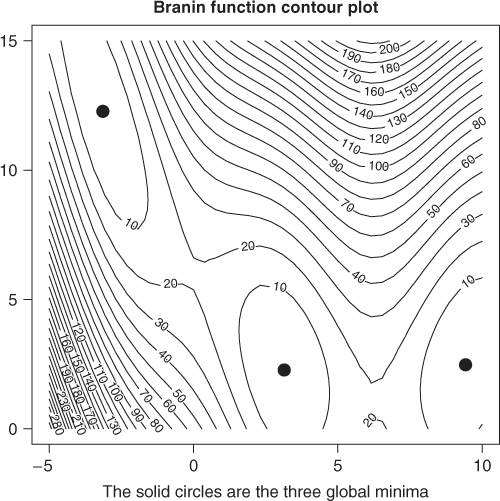
zz <- branin(pnts)
zz <- as.numeric(as.matrix(zz))
zy <- matrix(zz, nrow = 40, ncol = 40)
contour(grid1, grid2, zy, nlevels = 25)
points(y1[1], y1[2], pch = 19, cex = 2)
points(y2[1], y2[2], pch = 19, cex = 2)
points(y3[1], y3[2], pch = 19, cex = 2)
title(main = "Branin function contour plot")
title(sub = "The solid circles are the three global minima")
Now display the results.
for (ii in 1:npt) {
    vrow <- paste(cmat[ii, ], sep = " ", collapse = " ")
    cat(vrow, "
")
}
## 1 1 1 1 1 1 1 1 1 1 1 1 1 1 2 2 2 2 1 1 2 2 2 2 2 2 2 3 3 0 3 3 3 3 3 3 3 3 3 3
## 1 1 1 1 1 1 1 1 1 1 1 1 1 0 2 2 2 1 1 2 2 2 2 2 2 2 2 3 0 0 3 3 3 3 3 3 3 3 3 3
## 1 1 1 1 1 1 1 1 1 1 1 1 1 3 2 2 1 1 1 2 1 2 2 2 2 2 2 3 3 0 3 3 3 3 3 3 3 3 3 3
## 1 1 1 1 1 1 1 1 1 1 1 1 1 2 2 2 1 1 1 2 1 2 2 2 2 2 2 3 2 0 3 3 3 3 3 3 3 3 3 3
## 1 1 1 1 1 1 1 1 1 1 1 1 1 2 2 1 1 1 1 1 1 2 2 2 2 2 2 3 0 0 3 3 3 3 3 3 3 3 3 3
## 1 1 1 1 1 1 1 1 1 1 1 1 1 2 0 1 1 1 1 1 3 2 2 2 2 2 2 3 3 0 3 3 3 3 3 3 3 3 3 3
## 1 1 1 1 1 1 1 1 1 1 1 1 1 1 0 1 1 1 1 2 2 2 2 2 2 2 2 3 3 0 3 3 3 3 3 3 3 3 3 3
## 1 1 1 1 1 1 1 1 1 1 1 1 1 1 1 1 1 1 1 1 2 2 2 2 2 2 2 3 3 0 3 3 3 3 3 3 3 3 3 3
## 1 1 1 1 1 1 1 1 1 1 1 1 1 1 1 1 1 1 1 1 2 2 2 2 2 2 2 3 2 0 3 3 3 3 3 3 3 3 3 3
## 1 1 1 1 1 1 1 1 1 1 1 1 1 1 1 1 1 1 1 2 2 2 2 2 2 2 2 3 3 0 3 3 3 3 3 3 3 3 3 3
## 1 1 1 1 1 1 1 1 1 1 1 1 1 1 1 1 1 1 1 2 2 2 2 2 2 2 2 2 3 0 3 3 3 3 3 3 3 3 3 3
## 1 1 1 1 1 1 1 1 1 1 1 1 1 1 1 1 1 1 2 2 2 2 2 2 2 2 2 2 3 2 3 3 3 3 3 3 3 3 3 3
## 1 1 1 1 1 1 1 1 1 1 1 1 1 1 1 1 1 1 2 2 2 2 2 2 2 2 2 2 3 2 3 3 3 3 3 3 3 3 3 3
## 1 1 1 1 1 1 1 1 1 1 1 1 1 1 1 1 1 0 2 2 2 2 2 2 2 2 3 2 3 2 3 3 3 3 3 3 3 3 3 3
## 1 1 1 1 1 1 1 1 1 1 1 1 1 1 1 1 1 2 2 2 2 2 2 2 2 2 2 2 3 2 3 3 3 3 3 3 3 3 3 3
## 1 1 1 1 1 1 1 1 1 1 1 1 1 1 1 1 1 2 2 2 2 2 2 2 2 2 2 2 3 2 3 3 3 3 3 3 3 3 3 3
## 1 1 1 1 1 1 1 1 1 1 1 1 1 1 1 1 0 2 2 2 2 2 2 2 2 2 2 2 3 2 3 3 3 3 3 3 3 3 3 3
## 1 1 1 1 1 1 1 1 1 1 1 1 1 1 1 1 2 2 2 2 2 2 2 2 2 2 2 2 3 2 3 3 3 3 3 3 3 3 3 3
## 3 1 1 1 1 1 1 1 1 1 1 1 1 1 1 0 2 2 2 2 2 2 2 2 2 2 2 2 3 2 3 3 3 3 3 3 3 3 3 3
## 3 1 1 1 1 1 1 1 1 1 1 1 1 1 1 2 2 2 3 2 2 2 2 2 2 2 2 2 0 2 3 3 3 3 3 3 3 3 3 3
## 3 3 1 1 1 1 1 1 1 1 1 1 1 1 0 2 2 2 3 2 2 2 2 2 2 2 2 2 3 2 3 3 3 3 3 3 3 3 3 3
## 3 3 1 1 1 1 1 1 1 1 1 1 1 1 2 2 2 2 2 2 2 2 2 2 2 2 2 2 3 2 3 3 3 3 3 3 3 3 3 3
## 3 3 3 1 1 1 1 1 1 1 1 1 0 1 2 2 2 2 2 3 2 2 2 2 2 2 2 2 0 2 3 3 3 3 3 3 3 3 3 3
## 3 3 3 3 1 1 1 1 1 1 1 0 1 1 0 2 2 2 2 2 2 2 2 2 2 2 2 2 3 2 3 3 3 3 3 3 3 3 3 3
## 3 3 3 3 1 1 1 1 1 1 1 0 0 0 2 0 2 2 2 2 2 2 2 2 2 2 2 2 3 2 3 3 3 3 3 3 3 3 3 3
## 3 3 3 3 3 1 1 2 1 1 1 1 1 2 2 0 2 2 2 2 2 2 2 2 2 2 2 2 3 2 3 3 3 3 3 3 3 3 3 3
## 3 3 3 3 3 1 1 2 0 1 1 1 0 2 0 3 0 0 2 2 2 2 2 2 2 2 2 2 2 2 3 3 3 3 3 3 3 3 3 3
## 3 3 3 3 3 3 1 0 0 1 1 1 2 2 2 3 3 3 0 2 2 2 2 2 2 2 2 2 2 2 3 3 3 3 3 3 3 3 3 3
## 3 3 3 3 3 3 0 0 2 0 2 2 3 2 3 3 3 3 3 2 2 2 2 2 2 2 2 2 2 2 3 3 3 3 3 3 3 3 3 3
## 3 3 3 3 3 3 3 2 2 2 2 0 3 2 3 3 3 3 3 2 2 2 2 2 2 2 2 2 2 2 3 3 3 3 3 3 3 3 3 3
## 3 3 3 3 3 3 3 3 2 2 0 3 3 3 3 3 3 3 3 2 2 2 2 2 2 2 2 2 2 2 3 3 3 3 3 3 3 3 3 3
## 3 3 3 3 3 3 3 3 2 0 3 3 3 3 3 3 3 3 3 3 2 2 2 2 2 2 2 2 2 2 3 3 3 3 3 3 3 3 3 3
## 3 3 3 3 3 3 3 3 2 3 3 3 3 3 3 3 3 3 3 3 2 2 2 2 2 2 2 2 0 2 3 3 3 3 3 3 3 3 3 3
## 3 3 3 3 3 3 3 3 3 3 3 3 3 3 3 3 3 3 3 3 2 2 2 2 2 2 2 2 0 2 3 3 3 3 3 3 3 3 3 3
## 3 3 3 3 3 3 3 3 3 3 3 3 3 3 3 3 3 3 3 3 2 2 2 2 2 2 2 2 0 0 3 3 3 3 3 3 3 3 3 3
## 3 3 3 3 3 3 3 3 3 3 3 3 3 3 3 3 3 3 3 3 2 2 2 2 2 2 2 2 0 0 3 3 3 3 3 3 3 3 3 3
## 3 3 3 3 3 3 3 3 3 3 3 3 3 3 3 3 3 3 3 3 3 2 2 2 2 2 2 2 0 0 0 3 3 3 3 3 3 3 3 3
## 3 3 3 3 3 3 3 3 3 3 3 3 3 3 3 3 3 3 3 3 3 2 2 2 2 2 2 2 0 0 0 3 3 3 3 3 3 3 3 3
## 3 3 3 3 3 3 3 3 3 3 3 3 3 3 3 3 3 3 3 3 3 2 2 2 2 2 2 2 0 0 0 3 3 3 3 3 3 3 3 3
## 3 3 3 0 3 3 3 3 3 3 3 3 3 3 3 3 3 3 3 3 3 2 2 2 2 2 2 2 2 0 0 3 3 3 3 3 3 3 3 3
References
- Adragni KP, Cook RD, and Wu S 2012 GrassmannOptim: an R package for Grassmann manifold optimization. Journal of Statistical Software 50(5), 1–18.
- based on the work of Ivan Zelinka JC 2011 soma: General-purpose optimisation with the Self-Organising Migrating Algorithm. R package version 1.1.0.
- Bergmeir C, Molina D, and Benítez JM 2012 Continuous Optimization using Memetic Algorithms with Local Search Chains (MA-LS-Chains) in R. R package version 0.1.
- de Colombia PJDVHUN 2012 smco: A simple Monte Carlo optimizer using adaptive coordinate sampling. R package version 0.1.
- Eddelbuettel D 2012 RcppDE: Global optimization by differential evolution in C++. R package version 0.1.1. Extends DEoptim which itself is based on DE-Engine (by Rainer Storn).
- Mebane WR Jr. and Sekhon JS 2011 Genetic optimization using derivatives: the rgenoud package for R. Journal of Statistical Software 42(11), 1–26.
- Molga M and Smutnicki C 2005 Test functions for optimization needs.
- Mühlenbein H, Schomisch D, and Born J 1991 The parallel genetic algorithm as function optimizer. Parallel Computing 17(6-7), 619–632.
- Mullen K, Ardia D, Gil D, Windover D, and Cline J 2011 DEoptim: an R package for global optimization by differential evolution. Journal of Statistical Software 40(6), 1–26.
- Murphy L 2012 Likelihood: Methods for maximum likelihood estimation. R package version 1.5.
- Scrucca L 2013 GA: a package for genetic algorithms in R. Journal of Statistical Software 53(4), 1–37.
- Tenorio F 2013 Gaoptim: Genetic Algorithm optimization for real-based and permutation-based problems. R package version 1.1.
- Törn A and Zilinskas A 1989 Global Optimization, Lecture Notes in Computer Science. New York: Springer-Verlag.
- Xiang Y, Gubian S, Suomela B, and Hoeng J 2013 Generalized simulated annealing for global optimization: the gensa package for r. The R Journal 5(1), 13–29.