20.1 The model

The description here refers directly to the program code below. The model aims to explain the numbers of susceptible (S), infected (I), and recovered (R) in a cholera outbreak. The particular model includes a variable that measures bacteria concentration in water (). This leads to the SIWR model developed by Tien and Earn 2010, Bi and Bw are parameters that describe the direct (human–human) and indirect (waterborne) cholera transmission. e is the pathogen decay rate in the water.

We do not measure I directly, but a scaled version of it

y = I/k

where k is a combination of the reporting rate, the asymptomatic rate, and the total population size.

Our equations include a recovery rate and a birth–death parameter, but in the present situation, the description of the problem states that the former is fixed at 0.25 and the latter is 0.

Unfortunately, the code suggested fails to do a good job of optimizing the cost function. An e-mail exchange between myself and Nathan Lemoine that prompted this investigation was initiated with his blog posting http://www.r-bloggers.com/evaluating-optimization-algorithms-in-matlab-python-and-r/.

20.2 Background

Ecological models that involve multiple differential equations are common. They are closely related to compartment models for pharmacokinetics and chemical engineering.

The motivating problem involves a series of measurements for different time points. Unfortunately, after this section was written, we realized that the data set used had not been formally released for use, so I have replaced it with a similar set of data that has been generated by loosely drawing a similar picture and “guesstimating” the numbers from that graph.

The variable data is observed for time tspan. We load the package deSolve and establish the ordinary differential equations (ODEs) in the function SIRode. Some housekeeping matters include merging the model parameters into a vector (params) and specifying initial conditions for the differential equations that depend on one of these parameters (k). Noting that the initial guess to parameter k is very small, it is sensible to work with a scaled parameter, and our choice is to use 1e+5*k as the quantity to estimate. Moreover, e is initially set at 0.01, so let us use 100*e as the quantity to optimize.

The suitability and motivations for the present model will not be argued here. These are important matters, but they are somewhat separate from the estimation task.

tspan <- c(0, 8, 13, 20, 29, 34, 41, 50, 56, 62, 71, 78, 83, 91, 99, 104, 111,
    120, 127, 134, 139, 148, 155, 160)
data <- c(115, 59, 69, 142, 390, 2990, 4700, 5488, 5620, 6399, 5388, 4422,
    3566, 2222, 1911, 2111, 1733, 1166, 831, 740, 780, 500, 540, 390)
## Main code for the SIR model example
require(deSolve)  # Load the library to solve the ode
## Loading required package: deSolve
## initial parameter values ##
Bi <- 0.75
Bw <- 0.75
e <- 0.01
k <- 1/89193.18
## define a weight vector OUTSIDE LLode function
wts <- sqrt(sqrt(data))
## Combine parameters into a vector
params <- c(Bi, Bw, e * 100, k * 1e+05)
names(params) <- c("Bi", "Bw", "escaled", "kscaled")
## ODE function ##
SIRode <- function(t, x, params) {
    S <- x[1]
    I <- x[2]
    W <- x[3]
    R <- x[4]
    Bi <- params[1]
    Bw <- params[2]
    e <- params[3] * 0.01
    k <- params[4] * 1e-05
    dS <- -Bi * S * I - Bw * S * W
    dI <- Bi * S * I + Bw * S * W - 0.25 * I
    dW <- e * (I - W)
    dR <- 0.25 * I
    output <- c(dS, dI, dW, dR)
    list(output)
}
## initial conditions ##
I0 <- data[1] * k
R0 <- 0
S0 <- (1 - I0)
W0 <- 0
initCond <- c(S0, I0, W0, R0)

Let us use the initial parameter guesses above and solve the ODEs using a particular method (Runge–Kutta(4,5) method) which is suitable for a fairly wide range of differential equations. We will graph the data and the model that use the parameter guesses (Figure 20.1), where the dashed line is the model.

## Run ODE using initial parameter guesses ##
initSim <- ode(initCond, tspan, SIRode, params, method = "ode45")
plot(tspan, initSim[, 3]/k, type = "l", lty = "dashed")
points(tspan, data)

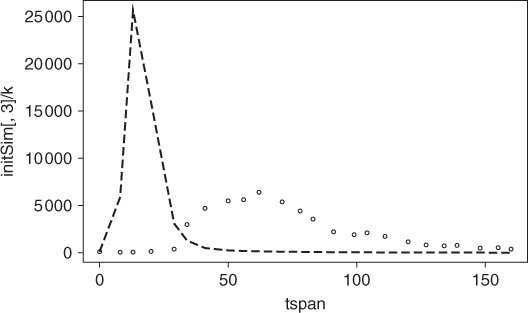
Clearly, the model does not come close enough to the data to be useful. We have some improvements to make in the parameter values.

There is also the possibility that we could use a different integrator for the differential equations. What is the justification for choosing the Runge–Kutta(4, 5) method? Admittedly, this is a popular and reliable method, and its wide use attests to its general strength. However, there is also the LSODA solver that is intended to balance between stiff and nonstiff solvers, as well as a number of other choices. In this area, I count myself essentially a novice. In the following function LLode, ode45 is used, as suggested in the original script sent to me.

20.3 The likelihood function

The suggested solution involves maximizing the likelihood or, for our purposes, minimizing the negative log likelihood. Let us first define this. In the present case, it is no more than a weighted sum of squares. However, to get the model, we need to solve the differential equations repeatedly. Moreover, the original code discussed in the blog that motivated this article did not check the diagnostic flags of the solver. We now do that. Note that the value of the flag may change according to the solver selected within the deSolve package.

It is arguable that the decision to allow different “success” code values is inviting users to get into trouble. The reason is probably that the codes assembled together and wrapped into deSolve return these codes, and it is useful for the developer to compare results from the wrapper with those from the original code in its original programming language.

## Define likelihood function using weighted least squares ##
LLode <- function(params) {
    k <- params[4] * 1e-05
    I0 <- data[1] * k
    R0 <- 0
    S0 <- 1 - I0
    W0 <- 0
    initCond <- c(S0, I0, W0, R0)
    # Run the ODE
    odeOut <- ode(initCond, tspan, SIRode, params, method = "ode45")
    if (attr(odeOut, "istate")[1] != 0) {
        ## Check if satisfactory 2 indicates perceived success of        method 'lsoda', 0 for
        ## 'ode45'.  Other integrators may have different indicator codes
        cat("Integration possibly failed
")
        LL <- .Machine$double.xmax * 1e-06  # indicate failure
    } else {
        y <- odeOut[, 3]/k  # Measurement variable
        wtDiff <- (y - data) * wts  # Weighted difference
        LL <- as.numeric(crossprod(wtDiff))  # Sum of squares
    }
    LL
}

20.4 A first try at minimization

Let us try to minimize this function using R's optim(), which will invoke the Nelder–Mead method by default, although we make the call explicit in the following. We could use trace=1 to observe the minimization.

## optimize using optim() ##
MLoptres <- optim(params, LLode, method = "Nelder-Mead",     control = list(trace = 0,   maxit = 5000))
MLoptres
## $par
##       Bi       Bw  escaled  kscaled
## 0.307331 1.142383 0.453779 0.965853
##
## $value
## [1] 208064645
##
## $counts
## function gradient
##      221       NA
##
## $convergence
## [1] 0
##
## $message
## NULL

We note a considerably better fit to the data with the optimized parameters, and this is reflected in Figure 20.2 (solid line), where we include the model using the preliminary guesses to the parameters (dotted line).

20.5 Attempts with optimx

Let us try some methods in the package optimx. We now add some bounds to the parameters and choose two methods that are suitable for bounds and do not need derivatives. After this, we see that there is a very small—almost invisible—improvement in the model. As this computation is quite slow—look at the timings displayed with the optimizers in column xtimes—we ran this off-line and saved the result using the R command dput().

require(optimx)
optxres <- optimx(params, LLode, lower = rep(0, 4), upper = rep(500, 4), method = c("nmkb", "bobyqa"), control = list(usenumDeriv = TRUE, maxit = 5000, trace = 0))
summary(optxres, order = value)
## dput(optxres, file='includes/C20opresult.dput')
bestpar <- coef(summary(optxres, order = value)[1, ])
cat("best parameters:")
print(bestpar)
## dput(bestpar, file='includes/C20bestpar.dput')
bpSim <- ode(initCond, tspan, SIRode, bestpar, method = "ode45")
X11()
plot(tspan, initSim[, 3]/k, type = "l", lty = "dashed")
points(tspan, data)
points(tspan, MLSim[, 3]/k, type = "l", lty = "twodash")
points(tspan, bpSim[, 3]/k, type = "l")
title(main = "Improved fit using optimx")

## from running supportdocs/ODEprobs/ODElemoine.R
optxres <- dget("includes/C20opresult.dput")
optxres
##               Bi        Bw  escaled    kscaled       value fevals gevals niter
## bobyqa 0.3060053   1.87848 0.283434   0.981722   207751806   5000     NA    NA
## nmkb   0.0352253 493.81805 3.061697 114.234193 14907264560    585     NA    NA
##        convcode  kkt1  kkt2  xtimes
## bobyqa        0 FALSE FALSE  29.010
## nmkb          0 FALSE FALSE 104.606
bestpar <- dget("includes/C20bestpar.dput")

20.6 Using nonlinear least squares

Given the form of the likelihood, we could use a nonlinear least squares method. Here is the residual function.

Lemres <- function(params) {
    k <- params[4] * 1e-05
    I0 <- data[1] * k
    R0 <- 0
    S0 <- 1 - I0
    W0 <- 0
    initCond <- c(S0, I0, W0, R0)
    nobs <- length(tspan)
    resl <- rep(NA, nobs)
    # Run the ODE
    odeOut <- ode(initCond, tspan, SIRode, params, method = "ode45")
    if (attr(odeOut, "istate")[1] != 0) {
        ## Check if satisfactory
        cat("Integration possibly failed
")
        resl <- rep(.Machine$double.xmax * 1e-12, nobs)
    } else {
        y <- odeOut[, 3]/k
        resl <- (y - data) * wts
    }
    resl
}

Now we will run the nonlinear least squares minimizer.

## Loading required package: nlmrt
## nlmrt class object: x
## residual sumsquares =  218712359  on  24 observations
##     after  15    Jacobian and  24 function evaluations
##   name       coeff       SE      tstat      pval      gradient    JSingval
## Bi         0.330594    0.01157     28.59          0   2.134e+09     2102404
## Bw         0.146237    0.07912     1.848    0.07939    80497932      234087
## escaled     1.26505      2.152    0.5878     0.5632    12993872       44584
## kscaled    0.739756    0.09626     7.685  2.157e-07   -97353705        1535

This is not as good a result as the best so far obtained, so we will not pursue it further.

20.7 Commentary

There are several ideas that are important to obtaining a decent solution with reasonable efficiency:

• It appears to be important to check if the differential equation integration was successful. An awkwardness in doing so is the fact that different methods in deSolve use different values of the flag to indicate success or lack thereof.
• Bounds may be useful in keeping parameters in a particular range, that is, positive, but may slow down the solution process.

The following are some points to consider:

• Is it worth figuring out how to generate analytic derivative information? This may be a quite difficult task.
• Should we bother with gradient methods when we do not have analytic gradients for problems such as this?
• Is our code more comprehensible if we explicitly include the exogenous tspan and data in the dot variables?

While we have found solutions here, it appears that drastically different sets of model parameters give rise to similar fits, as can be partly seen from the following table. This is a concern, as we then have to worry about the meaning of our parameters. That they are not well defined suggests that the model structure needs adjustment, rather than the solution method.

## Function value LLode * 1e-8 and parameters
## Guess,        223.44
##      Bi      Bw escaled kscaled
##  0.7500  0.7500  1.0000  1.1212
## ML - Nelder,  2.0806
##      Bi      Bw escaled kscaled
## 0.30733 1.14238 0.45378 0.96585
## Optimx-best,  2.0775
##             Bi     Bw escaled kscaled
## bobyqa 0.30601 1.8785 0.28343 0.98172
## nlfb-nlls,    2.1871
##      Bi      Bw escaled kscaled
## 0.33059 0.14624 1.26505 0.73976
## attr(,"pkgname")
## [1] "nlmrt"

Reference

1. Tien JH and Earn DJD 2010 Multiple transmission pathways and disease dynamics in a waterborne pathogen model. Bulletin of Mathematical Biology 72(6), 1506–1533.