2.1 Methods that use the gradient

If we seek a single (local) minimum of a function , possibly subject to constraints, one of the most obvious approaches is to compute the gradient of the function and proceed in the reverse direction, that is, proceed “downhill.” The gradient is the -dimensional slope of the function, a concept from the differential calculus, and generally a source of anxiety for nonmathematics students.

Gradient descent is the basis of one of the oldest approaches to optimization, the method of steepest descents (Cauchy, 1848). Let us assume that we are at point (which will be a vector if we have more than one parameter) where our gradient—the vector of partial derivatives of the objective with respect to each of the parameters—is . The method is then to proceed by a sequence of operations where we find a “lower” point at

2.1

The “minor detail” of choosing is central to a workable method, and in truth, the selection of a step length in descent methods is a serious topic that has filled many journals.

While the name sounds good, steepest descents generally is an inefficient optimization method in parameters. A version of steepest descents was created by simplifying the Rcgmin package. Let us try minimizing a function that is the sum of squares

2.2

which is expressed in R, along with its gradient as follows:

sq.f <- function(x) {
    nn <- length(x)
    yy <- 1:nn
    f <- sum((yy - x)^2)
    cat(“Fv=”, f, “ at ”)
    print(x)
    f
}
sq.g <- function(x) {
    nn <- length(x)
    yy <- 1:nn
    gg <- 2 * (x - yy)
}

This function is quite straightforward to minimize with steepest descents from most starting points. Let us use . (We will discuss more about starting points later. See Section 18.2.)

source(“supportdocs/steepdesc/steepdesc.R”)
# note location of routine in directory under nlpor
x <- c(0.1, 0.8)
asqsd <- stdesc(x, sq.f, sq.g, control = list(trace = 1))
## stdescu -- J C Nash 2009 - unconstrained version CG min
## Fv= 2.25  at [1] 0.1 0.8
## Initial function value= 2.25
## Initial fn= 2.25
## 1   0   1   2.25   last decrease= NA
## Fv= 2.237  at [1] 0.1027 0.8036
## Fv= 8.4e-23  at [1] 1 2
## 3   1   2   8.4e-23   last decrease= 2.25
## Very small gradient -- gradsqr = 3.36016730417128e-22
## stdesc seems to have converged
print(asqsd)
## $par
## [1] 1 2
##
## $value
## [1] 8.4e-23
##
## $counts
## [1] 3 2
##
## $convergence
## [1] 0
##
## $message
## [1] "stdesc seems to have converged"

However, a nonparabolic function is more difficult. From the same start, let us try the well-known Rosenbrock function, here stated in a generalized form. We turn off the trace, as the steepest descent method uses many function evaluations.

# ls() 1 to (n-1) variant of generalized rosenbrock function
grose.f <- function(x, gs = 100) {
    n <- length(x)
    1 + sum(gs * (x[1:(n - 1)] - x[2:n]^2)^2 + (x[1:(n - 1)] - 1)^2)
}
grose.g <- function(x, gs = 100) {
    # gradient of 1 to (n-1) variant of generalized rosenbrock function
    # vectorized by JN 090409
    n <- length(x)
    gg <- as.vector(rep(0, n))
    tn <- 2:n
    tn1 <- tn - 1
    z1 <- x[tn1] - x[tn]^2
    z2 <- x[tn1] - 1
    gg[tn1] <- 2 * (z2 + gs * z1)
    gg[tn] <- gg[tn] - 4 * gs * z1 * x[tn]
    gg
}
x <- c(0.1, 0.8)
arksd <- stdesc(x, grose.f, grose.g, control = list(trace = 0))
print(arksd)
## $par
## [1] 0.9183 0.9583
##
## $value
## [1] 1.007
##
## $counts
## [1] 502 199
##
## $convergence
## [1] 1
##
## $message
## [1] "Too many function evaluations (> 500) "

We will later see that we can do much better on this problem.

2.2 Newton-like methods

Equally if not more historic is Newton's method. The original focus was on finding the roots of functions, and the optimization version attempts to provide the step toward the minimum by approximately solving for the point at which the gradient will be zero. That is, we do not directly optimize but try to find the location of the valley bottom where there is no slope. There is some debate over where and when the method was actually published, and I will not add to this here. Richard Anstee gives a useful historical discussion at the end of his tutorial www.math.ubc.ca/~anstee/math184/184newtonmethod.pdf.

Certainly, anything similar to a modern view of the method was not used by Newton or Raphson, whose names are often linked to it.

The modern view of the method is as follows. In one dimension, we start at point and compute the gradient and second derivative . We then solve for

2.3

and repeat the process from

2.4

Let us try this from with the function

2.5

F <- function(x) exp(-0.05 * x) * (x - 4)^2
curve(F, from = 0, to = 5)
newt <- function(x) {
    xnew <- x - (exp(-0.05 * x) * (2 * (x - 4)) - exp(-0.05 * x) * 0.05
        * (x - 4)^2)/(exp(-0.05 * x) * 2 - exp(-0.05 * x) * 0.05 *
        (2 * (x - 4)) - (exp(-0.05 * x) * 0.05 * (2 * (x - 4))
        - exp(-0.05 * x) * 0.05 * 0.05 * (x - 4)^2))
}
x <- 1
xold <- 0
while (xold != x) {
    xold <- x
    cat("f(", x, ")=", F(x), "
")
    x <- newt(xold)
}
## f( 1 )= 8.561
## f( 3.459 )= 0.2457
## f( 3.979 )= 0.0003603
## f( 4 )= 8.871e-10
## f( 4 )= 5.407e-21
## f( 4 )= 0

A warning: If you read articles about Newton's method that view it as root-finding, say of function , then the iteration equation is in the form of

2.6

Thus the optimization view requires two degrees of derivatives of the original function . This is a serious amount of mental effort in most problems.

The -parameter Newton method uses the Hessian matrix of second derivatives of the objective function with respect to the parameters, which is the generalization of the second derivative for the 1D problem above. Starting at some set of parameters , we compute H and . We then solve

2.7

and try to compute the objective

2.3 The promise of Newton's method

Newton's method is attractive because there are theoretical results that show it is extremely efficient under some conditions that are not too unlikely. Principally, the quality of Newton's method that is attractive is quadratic convergence, which means that if we are “close enough” to a solution with our starting estimate , then after some iterations, the distances to the solution will obey

2.8

A statement that is easier to understand is that the number of correct digits approximately doubles with each iteration. This is more or less what is seen in the earlier example, in which convergence is very rapid.

2.4 Caution: convergence versus termination

This is a good point to make the first of what will be several mentions that the theoretical concept of the convergence of iterative algorithms can be very important for understanding them, but it may be quite unlike the actual termination of the program implementing that algorithm.

Algorithms converge; programs terminate.

We generally need to put in very carefully considered tests and conditions to ensure that we do, in fact, terminate (Nash, 1987).

It is useful to be a bit persnickety and insist on keeping “convergence” for algorithms or methods and “termination” for their implementations because this will remind us that the programs have to deal with situations that are outside the purview of the mathematical niceties. For example, it is very easy in this era of “cut and paste” to get character formatting information into what looks like a simple number, giving some sort of error as our optimization code misinterprets the information we are supplying.

2.5 Difficulties with Newton's method

There are lots of dangerous beasts in the night-time optimization forest. Most of these can be seen in one-parameter problems, but it is worth noting that dimensions usually make things a lot more difficult, because the issues have essentially an -fold possibility of occurrence. The Wikipedia article http://en.wikipedia.org/wiki/Newton's_method presents these issues very clearly, along with a lot of other well-prepared material. These difficulties can be overcome with careful attention to detail. We list the main issues here, illustrated in one dimension:

• singular Hessian, for example, ;
• multiple minima, for example, ;
• constraints, for example, subject to ;
• undefined function, for example, when approaches 0;
• too big a step, for example, with a step bigger than which will move the parameter to the next trigonometric cycle.

2.6 Least squares: Gauss–Newton methods

Statisticians often deal with problems that involve objective functions that are sums of squares. The classic linear regression and analysis of variance tools of multivariate statistics minimize sums of squared residuals, although most users of the lm() linear modeling function in R would not necessarily have that viewpoint. Moreover, there are a number of situations in which the traditional problem is modified so that either the parameter estimates or other quantities are constrained. In such cases, other tools are needed. Sometimes an optimization tool can be a practical approach to finding a solution.

As with its linear counterpart, the nonlinear least squares problem is so common that special methods have been developed and should be considered when such problems are to be solved. There is a huge literature, and many factional disputes on how things should be done.

The main approach—and one that is used in R's nls() function—is the Gauss–Newton method. Our objective function is the sum of nobs squared elements that we may consider as residuals. If we have a model data) that involves our parameters and some other data to model a variable (here explicitly written as a vector of observations), we can write the nobs residuals as

2.9

This is the “wrong way round” for most statisticians, including Gauss, but because we are squaring the residuals, the objective function is the same. I like this way because the derivatives of the residuals and the model then have the same sign, and sign errors are so common that I do everything I can to avoid them. If you are happier with the conventional “data-model” formulation, please feel free to use it. This is a matter of preference, not law.

If we try to apply the Newton method to a nonlinear least squares problem, we see that the gradient of the objective function is

2.10

where

2.11

gives the element of the Jacobian of the residuals with respect to .

However, the Hessian is now more complicated,

2.12

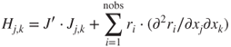
The second part of this expression involving the second partial derivatives of the residuals is generally “ignored” on the basis that the residuals are usually “small.” This is, of course, an interesting twist on the argument that nls is not useful for small residual problems. The practical reason is that these derivatives require us to compute nobs square matrices each of a size equal to the number of parameters—a big chore.

A very successful “cheat” is to approximate the second term with some other matrix. Donald Marquardt (Marquardt, 1963) developed one of the most successful early nonlinear least squares codes by adding a scaled unit matrix to the Jacobian inner product, that is,

2.13

The effect of this is that when is very large, we solve

2.14

and get a steepest descents search direction. When is small, we have the Gauss–Newton search direction. In practice, with a strategy that increases when we fail to reduce the sum of squares and decreases it when we succeed, this works very well. Of course, there are numerous discussions on the tactical details of the settings for increase, decrease, and initial . As far as I can determine, sometime after Marquardt's paper appeared, it was noted that the ideas had been suggested sometime during World War II by Levenberg 1944, and his name is sometimes added to the method.

Marquardt also showed that using a matrix instead of , defined

2.15

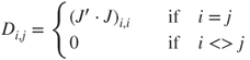
avoids some issues when the parameters are of widely different scale, as in the Hobbs weeds problem (see Section 1.2). However, when I came to that problem, I was working (in 1974) on a Data General NOVA in BASIC, where the floating point arithmetic used six hexadecimal digits without a guard digit. In computing the sum of squares and cross products , some of the diagonal elements underflowed to zero, which rendered the stabilization ineffective. I found that the unscaled version (using just an identity matrix ) worked, but even better was a combination

2.16

where is a smallish number (I generally use 1).

Other approaches abound, such as using a line search with the original Gauss–Newton method (Hartley, 1961) or solving the Gauss–Newton equations with a singular value decomposition and dropping directions that correspond to small singular values (Jones, 1970). My experience is that the Marquardt approach with attention to the possibility of underflow works as well as any other method and has the merit of simplicity.

2.7 Quasi-Newton or variable metric method

We have seen that Newton's method obtains a search direction from a solution of the equation

2.17

From this, many stabilized versions of Newton's method can be created using different strategies and tactics to search along and control for potential mishaps. However, the fundamental chore in Newton's method is computing the Hessian . Even the gradient is a considerable difficulty, but for the moment, we will take this as feasible.

As with the Gauss–Newton method, we will try to approximate in ways that are easier to compute. It can be argued that the most effective approach is the family of algorithms called quasi-Newton methods. These begin with an approximation either to or its inverse . The following are the steps of any of the quasi-Newton method, with some variants referred to as variable metric methods:

• Provide starting parameters , set an initial “approximate” Hessian or Hessian inverse, and compute the initial function and gradient , as well as any settings needed to control a particular method.
• “Solve” the Newton equations to get a search direction . For methods using an approximate Hessian inverse, this is simply a matrix multiplication. Other approaches may solve the equations explicitly, or else work with decompositions of the approximate Hessian or approximate Hessian inverse.
• Perform some kind of line search along the search direction . A failure to improve the function value is one component of the termination tests.
• Update the approximate Hessian or approximate Hessian inverse in some way. There are a number of approaches, but most are based on two families of update formulas, one labeled “Davidon Fletcher Powell” (DFP) and the other “Broyden–Fletcher–Goldfarb Shanno” (BFGS). However, there are many details that may be important.
• Apply various termination tests and possibly restart the process if progress is not being made.

To illustrate this, the “BFGS” method of optim() uses an identity matrix as the initial approximate inverse Hessian, so the first search direction is steepest descents. The line search simply shortens the step along this direction until a “satisfactory decrease” is found. This is sometimes called backtracking to an acceptable point. The BFGS formula is used to update the inverse Hessian approximation. If the line search is not successful, the inverse Hessian approximation is reset to the identity and we only terminate when the line search fails for this steepest descents direction.

The unconstrained optimizer Rvmminu from package Rvmmin is supposed to be the same algorithm, but I note that the sequence of evaluation points for some trial problems is not the same with this code and with optim ‘BFGS’. However, very small changes in arithmetic or control settings can alter trajectories of minimizers, so this is not totally surprising.

By comparison, the minimizer ucminf uses much the same approach but with a quadratic inverse interpolation line search (Nielsen, 2000). This appears to be slightly more efficient than optim method ‘BFGS’, and I have toyed with trying to implement it. However, the code and description are sufficiently complicated that I have not done so. My motive for reimplementing the method was to add bounds constraints (Chapter 11).

2.8 Conjugate gradient and related methods

A somewhat different approach to gradient-based function minimization is the family of nonlinear conjugate gradient minimizers. These are derived as if one is minimizing a quadratic form with the Hessian a constant positive definite matrix. This leads to an algorithm that has the following structure:

• Provide starting parameters , and compute the initial function and gradient . Choose the initial search direction to be the negative gradient.
• Perform some kind of line search along the search direction. A failure to improve the function value stops the method if we are searching along the negative gradient, or else we reset the search to this direction.
• We compute the gradient at the new point and use it, the previous gradient and the search direction to derive a new search direction. Note that this involves only a few vectors of storage. There are several formulas to update the search direction, and a number of tests to ensure that this is a “good” direction.
• Apply various termination or restart tests and continue until progress is not being made.

Despite the very low storage requirement and rather simple structure of CG methods, they often perform surprisingly well on quite large problems (i.e., in hundreds of parameters). On the other hand, “often” is not the same as “almost always,” and it is important to note that I regard the ‘CG’ method in optim() and its precursor in Nash (1979) as the least successful of the methods I implemented. This offers a choice of three formulas for updating the search direction, namely, the original Fletcher–Reeves formula, one due to Polak and Ribière, or one due to Beale and Sorenson. The first of these is the default in optim(); however, the second is my reluctant preference.

Fortunately, we need not fuss with such choices, Dai and Yuan 2001 showed a way to combine the formulas and use them to provide a test of when to restart the iteration. This is implemented in package Rcgmin and appears to work well. There is more recent work by Hager and Zhang 2006 that may offer further improvement, but I have not had an opportunity to implement these ideas.

2.9 Other gradient methods

For a problem in parameters, a quasi-Newton method requires working storage for a matrix of order plus several vectors of the same order. A conjugate gradients method is much more space efficient—just a few vectors—but may not be as good at minimizing the function in a few evaluations. Thus many researchers have sought to find ways to get both time and space efficiencies by methods that are somehow intermediate between the two families. One of these is represented in optim, the Limited Memory BFGS method of Nocedal and colleagues (Zhu et al. 1997). Another is the inexact Newton method and truncated-Newton method (Nash, 2000b), where we solve the (linear) Newton equations partially, in particular for the truncated-Newton methods by approximate iterative methods such as conjugate gradients. There are many details in such methods that are sometimes critical for efficiency in finding the solution. Worse, in my experience, these details can result in very large improvements in the methods for some problems but be detrimental in others.

2.10 Derivative-free methods

When analytic derivatives are extremely difficult or impossible to provide, it is necessary to use methods that only depend on the function value. I would echo the sentiments expressed in Conn et al. 2009 that methods for derivative-free optimization are a necessity, but they should not be used if gradients are available.

2.11 Stochastic methods

When the objective function has many minima, and the global minimum is sought, stochastic methods are often attempted. There is a plethora of such methods. So many, in fact, that I suspect there may be several named methods that are actually the same algorithms.

Some of the many names are

• Simulated Annealing (Kirkpatrick et al. 1983)
• Taboo Search (Glover, 1989)
• Quantum annealing

  (http://en.wikipedia.org/wiki/Quantum_annealing)

• Probability Collectives (Rajnarayan et al. 2006)
• Reactive search optimization (http://www.reactive-search.org)
• Cross-entropy method (Boer et al. 2002)
• Random search, of which there are a number of approaches, one of the earliest by Bremmerman 1970
• Stochastic tunneling (Wenzel and Hamacher, 1999)
• Parallel tempering, also known as replica exchange MCMC sampling, (Geyer, 1991; Swendsen and Wang, 1986)
• Stochastic hill climbing or stochastic gradient descent (various workers appear to use these terms in conjunction with machine learning and genetic algorithms)
• (Particle) swarm algorithms (Kennedy and Eberhart, 1995)
• Evolutionary operation, begun in the 1950s by George Box for process optimization, which has influenced the development of other evolutionary algorithms
• Genetic algorithms, which are one form of evolutionary algorithms, with many contributions starting as early as the 1950s, but possibly established by Holland 1975.

In addition, of course, there are many user-developed approaches to stochastic optimization. If the number of local optima is small, then random starts to conventional minimizers is a common and often-effective strategy. For example, Varadhan and Gilbert (2009a) provide function multiStart in package BB.

The major source of dissatisfaction with stochastic approaches to optimization is that they lack any guarantee that they have succeeded. Truthfully, methods for global optimization with guarantees of success are elusive or difficult to use or both, otherwise they would have replaced the stochastic methods. For particular functional forms, we may be able to apply specialized methods such as Hompack (Watson et al. 1997) or interval analysis (Hansen and Walster, 2004), but most users will have difficulty in confirming that their problems fit the conditions required for such methods. There are also, to my knowledge, no packages for use of such techniques in R.

2.12 Constraint-based methods—mathematical programming

While R is weak in mathematical programming (MP) tools, it is important to know that there is a huge family of tools in the wider community for solving optimization problems that are primarily defined through the constraints that must be imposed on the parameters. The linear programming (LP) problem, where we wish to minimize a linear function of the parameters subject to a number of inequality constraints, often combined with nonnegativity conditions on the parameters, is one of the classical computational problems with a very large literature. The original Dantzig Simplex method is still a subject of interest (Nash, 2000).

When we have a quadratic objective function, but still linear inequalities, we have the quadratic programming (QP) problem. Linearly constrained least squares problems can, therefore, be solved by QP methods. More general MP problems, sometimes called nonlinear programming (NLP), can be very difficult to properly formulate and solve. They may have no solution, or multiple solutions, or the solver may fail to find an acceptable solution. However, methods are gradually being developed for some classes of problems of this type.

Convex optimization, where the objective and constraints are convex functions over the parameter space and the set of allowed parameters is also a closed convex set, provides a class of optimization problems that is at the same time quite useful yet without tools in R that are designed for their solution.

R also tends to deal much more with continuous (i.e.,‘real’) numbers, while many mathematical programming tasks concern choices, assignments, sequences, and other essentially discrete parameters that are handled better by integers.

References

1. Boer PTD, Kroese D, Mannor S and Rubinstein R 2002 A tutorial on the cross-entropy method. Annals of Operations Research 134, 19–67.
2. Bremmerman H 1970 A method for unconstrained global optimization. Mathematical Biosciences 9, 1–15.
3. Cauchy A 1848 Mthode gnrale pour la resolution des systmes dquations simultanes. Comptes Rendus de l'Acadmie des Sciences 27, 536–538.
4. Conn AR, Scheinberg K and Vicente LN 2009 Introduction to Derivative-Free Optimization. Society for Industrial and Applied Mathematics, Philadelphia, PA.
5. Dai YH and Yuan Y 2001 An efficient hybrid conjugate gradient method for unconstrained optimization. Annals of Operations Research 103(1–4), 33–47.
6. Geyer CJ 1991 Markov chain Monte Carlo maximum likelihood Computing Science and Statistics, Proceedings of the 23rd Symposium on the Interface, p. n.a.. American Statistical Association, New York.
7. Glover F 1989 Tabu search - part 1. ORSA Journal on Computing 1(2), 190–206.
8. Hager WW and Zhang H 2006 Algorithm 851: CG_DESCENT, a conjugate gradient method with guaranteed descent. ACM Transactions on Mathematical Software 32(1), 113–137.
9. Hansen ER and Walster GW 2004 Global Optimization Using Interval Analysis. MIT Press, Cambridge, MA.
10. Hartley HO 1961 The modified Gauss–Newton method for the fitting of non-linear regression functions by least squares. Technometrics 3, 269–280.
11. Holland JH 1975 Adaptation in Natural and Artificial Systems. University of Michigan Press, Ann Arbor, MI.
12. Hooke R and Jeeves TA 1961 “direct search” solution of numerical and statistical problems. Journal of the ACM 8(2), 212–229.
13. Joe H and Nash JC 2003 Numerical optimization and surface estimation with imprecise function evaluations. Statistics and Computing 13(3), 277–286.
14. Jones A 1970 Spiral—a new algorithm for non-linear parameter estimation using least squares. Computer Journal 13(3), 301–308.
15. Kelley CT 1997 Detection and remediation of stagnation in the Nelder–Mead algorithm using a sufficient decrease condition. SIAM Journal on Optimization 10, 43–55.
16. Kennedy J and Eberhart R 1995 Particle swarm optimization. Proceedings of IEEE International Conference on Neural Networks, 1995, Vol. 4, pp. 1942–1948.
17. Kirkpatrick S, Gelatt CD Jr. and Vecchi MP 1983 Optimization by simulated annealing. Science 220(4598), 671–680.
18. Levenberg K 1944 A method for the solution of certain non-linear problems in least squares. Quarterly of Applied Mathematics 2, 164–168.
19. Marquardt DW 1963 An algorithm for least-squares estimation of nonlinear parameters. SIAM Journal on Applied Mathematics 11(2), 431–441.
20. Nash JC 1979 Compact Numerical Methods for Computers: Linear Algebra and Function Minimisation. Adam Hilger, Bristol. Second Edition, 1990, Bristol: Institute of Physics Publications.
21. Nash JC 1987 Termination strategies for nonlinear parameter determination. In Proceedings of the Australian Society for Operations Research Annual Conference (ed. Kumar S), pp. 322–334, Melbourne, Australia.
22. Nash JC 2000a The Dantzig simplex method for linear programming. Computing in Science and Engineering 2(1), 29–31.
23. Nash SG 2000b A survey of truncated-Newton methods. Journal of Computational and Applied Mathematics 124, 45–59.
24. Nelder JA and Mead R 1965 A simplex method for function minimization. Computer Journal 7(4), 308–313.
25. Nielsen HB 2000 UCMINF - an algorithm for unconstrained, nonlinear optimization. Technical report, Department of Mathematical Modelling, Technical University of Denmark. Report IMM-REP-2000-18.
26. Rajnarayan D, Wolpert D and Kroo I 2006 Optimization under uncertainty using probability collectives. Proceedings of 11th AIAA/ISSMO Multidisciplinary Analysis and Optimization Conference, Portsmouth, VA. AIAA-2006-7033.
27. Swendsen RH and Wang JS 1986 Replica Monte Carlo simulation of spin glasses. Physical Review Letters 57, 2607–2609.
28. Torczon V 1995 Pattern search methods for nonlinear optimization. SIAG/OPT Views and News 6, 7–11.
29. Varadhan R and Gilbert P 2009 BB: an R package for solving a large system of nonlinear equations and for optimizing a high-dimensional nonlinear objective function. Journal of Statistical Software 32(4), 1–26.
30. Watson LT, Sosonkina M, Melville RC, Morgan AP and Walker HF 1997 Algorithm 777: Hompack90: a suite of fortran 90 codes for globally convergent homotopy algorithms. ACM Transactions on Mathematical Software 23(4), 514–549.
31. Wenzel W and Hamacher K 1999 Stochastic tunneling approach for global minimization of complex potential energy landscapes. Physical Review Letters 82, 3003–3007.
32. Zhu C, Byrd RH, Lu P and Nocedal J 1997 Algorithm 778: L-bfgs-b: fortran subroutines for large-scale bound-constrained optimization. ACM Transactions on Mathematical Software 23(4), 550–560.