
3
Double‐Integrator Model
In this chapter, we re‐discuss the class of formation controllers presented in Chapter 2 in the context of a slightly more refined model, viz., the double‐integrator model. We will follow the same format as the previous chapter for ease of correlation.
The double‐integrator model accounts for the agent acceleration by treating the agent as a point mass. Therefore, it can be considered a very simple dynamic model for omnidirectional robots. Given a system of ![]() agents, the equations of motion for the double‐integrator model are
agents, the equations of motion for the double‐integrator model are
where ![]() represents the velocity of the
represents the velocity of the ![]() th agent with respect to an Earth‐fixed coordinate frame,
th agent with respect to an Earth‐fixed coordinate frame, ![]() is the acceleration‐level control input, and
is the acceleration‐level control input, and ![]() is defined as in (2.1). Since the agent velocity is now a system state rather than the control input, the formation control laws in this chapter will be a function of the agent velocities in addition to the positions.
is defined as in (2.1). Since the agent velocity is now a system state rather than the control input, the formation control laws in this chapter will be a function of the agent velocities in addition to the positions.
Note that the system transfer function matrix is now ![]() , which gives rise to the model name. Since the only difference between this transfer function and (2.2) is an additional integrator, the extension of the single‐integrator‐based control laws to (3.1) is rather seamless if one exploits the integrator backstepping methodology (see Appendix C.6).
, which gives rise to the model name. Since the only difference between this transfer function and (2.2) is an additional integrator, the extension of the single‐integrator‐based control laws to (3.1) is rather seamless if one exploits the integrator backstepping methodology (see Appendix C.6).
As in Section 2.1, we begin by deriving the distance error dynamics. To this end, we use (2.6) and (3.1a) to obtain

Differentiating (2.10) along 3.2 gives
where ![]() .
.
Given that ![]() in 3.3 cannot be directly prescribed since it is a system state, we follow the backstepping technique and introduce the following variable
in 3.3 cannot be directly prescribed since it is a system state, we follow the backstepping technique and introduce the following variable
where ![]() denotes the fictitious (or desired) velocity input, which will be specified later. The variable
denotes the fictitious (or desired) velocity input, which will be specified later. The variable ![]() quantifies the error between the actual agent velocity and the desired velocity‐level input. The design of
quantifies the error between the actual agent velocity and the desired velocity‐level input. The design of ![]() will be problem‐specific, and will come from the velocity‐level control laws of Chapter 2. That is, generally speaking,
will be problem‐specific, and will come from the velocity‐level control laws of Chapter 2. That is, generally speaking, ![]() where the superscript
where the superscript ![]() stands for one of the control input designs for the single‐integrator model. The block diagrams in Figure 3.1 illustrate the relationship between the control designs for the single‐ and double‐integrator models. As one can see, the velocity‐level, position control algorithms from Chapter 2 will be embedded in the acceleration‐level, velocity control loop to be designed in this chapter.
stands for one of the control input designs for the single‐integrator model. The block diagrams in Figure 3.1 illustrate the relationship between the control designs for the single‐ and double‐integrator models. As one can see, the velocity‐level, position control algorithms from Chapter 2 will be embedded in the acceleration‐level, velocity control loop to be designed in this chapter.

Figure 3.1Relationship between the (a) single‐ and (b) double‐integrator control designs.
Due to the new error variable 3.4, we introduce the augmented Lyapunov function candidate
where ![]() was defined in (2.10). Notice that
was defined in (2.10). Notice that ![]() is a potential energy‐like term since it is only position dependent, whereas
is a potential energy‐like term since it is only position dependent, whereas ![]() is a kinetic energy‐like term due to its dependence on velocity. Therefore,
is a kinetic energy‐like term due to its dependence on velocity. Therefore, ![]() captures the total energy of the double‐integrator model formation.
captures the total energy of the double‐integrator model formation.
After taking the time derivative of 3.5, we obtain

where 3.3, (3.1b), and 3.4 were used. Equation 3.6 is the analogue of (2.12) since it will be the starting point for all double‐integrator control designs as (2.12) was for the single‐integrator designs.
3.1 Cross‐Edge Energy
Before presenting the formation controllers, we need to discuss a complication in the stability analysis of the closed‐loop system that arises from the double‐integrator model. Specifically, this complication is related to the avoidance of flip ambiguities.
Recall that for the single‐integrator model, the position of the initial formation needs to be restricted to prevent convergence to a flip ambiguity since the velocity‐level control input is designed to promote convergence to Iso![]() or Amb
or Amb![]() , whichever is closer at
, whichever is closer at ![]() . Unfortunately, this condition is not sufficient for the double‐integrator model. In this case, the agents' velocity will also affect the convergence since it is a system state. This idea is conceptually illustrated by Figure 3.2. Note that even if the formation position is closer to Iso
. Unfortunately, this condition is not sufficient for the double‐integrator model. In this case, the agents' velocity will also affect the convergence since it is a system state. This idea is conceptually illustrated by Figure 3.2. Note that even if the formation position is closer to Iso![]() , the formation will overcome the energy barrier and converge to Amb
, the formation will overcome the energy barrier and converge to Amb![]() if its velocity is large enough. In other words, the total formation energy is now affected by the combination of potential energy and kinetic energy. The implication of this for stability is that a restriction also needs to be imposed on the initial velocity of the formation, which means that we need to limit the initial total energy of the formation.
if its velocity is large enough. In other words, the total formation energy is now affected by the combination of potential energy and kinetic energy. The implication of this for stability is that a restriction also needs to be imposed on the initial velocity of the formation, which means that we need to limit the initial total energy of the formation.

Figure 3.2Energy landscape where the formation is at position  with velocity
  .
.
While the need for an upper bound on the initial energy of the formation is evident, its precise value is difficult to calculate in general. For simple formations, one may be able to calculate a conservative value for the energy upper bound as illustrated next. Consider the desired triangular formation in Figure 3.3 along with one of its flipped versions. Note that a flip may occur whenever an agent has enough energy to cross the edge connecting the two other agents, e.g., agent 1 crossing edge ![]() . Once the agent crosses the edge, it is closer to Amb
. Once the agent crosses the edge, it is closer to Amb![]() and may be attracted to this undesired equilibrium. The question is then: What is the minimum energy needed for this to happen? Hereafter, we refer to this minimum energy as the cross‐edge energy,
and may be attracted to this undesired equilibrium. The question is then: What is the minimum energy needed for this to happen? Hereafter, we refer to this minimum energy as the cross‐edge energy, ![]() .
.

Figure 3.3Desired formation (solid line) and a flip ambiguity (dashed line).
A conservative estimate for the cross‐edge energy can be made by using the following observations: (i) the cross‐edge energy is related to the energy that drives the agents to a collinear formation and (ii) the minimum collinearity energy is given by the agent with the smallest distance to its cross‐edge, e.g., the dotted line in Figure 3.3. These rules facilitate the cross‐edge energy estimation because they are only position dependent. Furthermore, we have from 3.5 and (2.10) that ![]() , which is also only position dependent. That is, a sufficient condition for
, which is also only position dependent. That is, a sufficient condition for ![]() can be determined by calculating the minimum value of
can be determined by calculating the minimum value of ![]() when the three agents are collinear. For example, let
when the three agents are collinear. For example, let ![]() and
and ![]() . When agent 1 is collinear with agents 2 and 3, we have that
. When agent 1 is collinear with agents 2 and 3, we have that ![]() . For notational convenience, we use
. For notational convenience, we use ![]() where
where ![]() to denote that the agents are collinear. Therefore,
to denote that the agents are collinear. Therefore,

It can be found that the above function reaches a minimum at ![]() and
and ![]() . This means that if
. This means that if ![]() , the agents will not converge to the flip ambiguity.
, the agents will not converge to the flip ambiguity.
Notice that the condition ![]() imposes a trade‐off between the initial distance error and the initial velocity error. The larger the initial distance error, the smaller the initial velocity error needs to be, and vice versa. Based on 3.4, a small
imposes a trade‐off between the initial distance error and the initial velocity error. The larger the initial distance error, the smaller the initial velocity error needs to be, and vice versa. Based on 3.4, a small ![]() implies that the agents' velocities are close to
implies that the agents' velocities are close to ![]() , which is the desired velocity that ensures convergence to Iso
, which is the desired velocity that ensures convergence to Iso![]() .
.
For formations with ![]() , one may apply the above estimation method by triangulating the framework and comparing the cross‐edge energy of each triangle to estimate
, one may apply the above estimation method by triangulating the framework and comparing the cross‐edge energy of each triangle to estimate ![]() . For example, consider the infinitesimally rigid framework in Figure 3.4. The agents most likely to flip are agents 2 and 6 about cross‐edges
. For example, consider the infinitesimally rigid framework in Figure 3.4. The agents most likely to flip are agents 2 and 6 about cross‐edges ![]() and
and ![]() , respectively, since they only have two edges (constraints) each. Thus,
, respectively, since they only have two edges (constraints) each. Thus, ![]() where
where ![]() denotes the cross‐edge energy of agent
denotes the cross‐edge energy of agent ![]() . Note that higher order flips are also possible, but they would require more energy than aforementioned single‐agent flips. For example, agents
. Note that higher order flips are also possible, but they would require more energy than aforementioned single‐agent flips. For example, agents ![]() or
or ![]() could simultaneously also flip about cross‐edge
could simultaneously also flip about cross‐edge ![]() , or agents
, or agents ![]() could simultaneously flip about agent 1, leading to a full reflection of the formation.
could simultaneously flip about agent 1, leading to a full reflection of the formation.

Figure 3.4Triangulated hexagon framework.
3.2 Formation Acquisition
The formation acquisition controller for (3.1) will have the general form ![]() ,
, ![]() and
and ![]() where
where ![]() was defined in (1.2). Based on 3.6, the following theorem introduces the control law that solves the formation acquisition problem.
was defined in (1.2). Based on 3.6, the following theorem introduces the control law that solves the formation acquisition problem.
The expression for ![]() in 3.8 is given by
in 3.8 is given by
where from (1.15)
![]() ,
, ![]() , and from 3.3
, and from 3.3
The control 3.8–3.9 can be written element‐wise as

for ![]() and
and
This control is decentralized in the sense of Definition 1.1 since its implementation only requires each agent to measure its own velocity and the relative position and relative velocity to neighboring agents. The agent's velocity can be measured using onboard sensors such as an odometer and a compass.
3.3 Formation Maneuvering
The formation maneuvering control law for the double‐integrator model (3.1a)–(3.1b) is simply a combination of the designs in Sections 2.2 and 3.2. Specifically, ![]() is given by 3.8 with
is given by 3.8 with
where the formation maneuvering velocity ![]() was specified in (2.24). Note that 3.17 is exactly the right‐hand side of (2.23).
was specified in (2.24). Note that 3.17 is exactly the right‐hand side of (2.23).
We will not present the formal statement and proof of this result, but only discuss the aspects in which it differs from the proofs of Theorems 2.2 and 3.1. This is namely the proof that (1.28) holds. First, after substituting 3.17 into 3.6, the proofs of the exponentially stability of ![]() and (1.26) are straightforward given that
and (1.26) are straightforward given that ![]() (see (1.20) and (2.24)). Now, since
(see (1.20) and (2.24)). Now, since ![]() as
as ![]() , we know from (2.9) that
, we know from (2.9) that ![]() as
as ![]() . Since
. Since ![]() is bounded, then
is bounded, then ![]() as
as ![]() from (2.15). Therefore, we have that
from (2.15). Therefore, we have that ![]() as
as ![]() from 3.17. Since we know
from 3.17. Since we know ![]() as
as ![]() , it follows from 3.4 that
, it follows from 3.4 that ![]()
![]() as
as ![]() . Therefore,
. Therefore, ![]() as
as ![]() ,
, ![]() , which is the same as (1.28) due to (3.1a).
, which is the same as (1.28) due to (3.1a).
The term ![]() in 3.8 will contain additional terms from the derivative of
in 3.8 will contain additional terms from the derivative of ![]() . Specifically, from (2.24), we have that
. Specifically, from (2.24), we have that
where ![]() denotes the desired translational acceleration and
denotes the desired translational acceleration and ![]() is the desired angular acceleration for the virtual rigid body. Therefore, for the double‐integrator model,
is the desired angular acceleration for the virtual rigid body. Therefore, for the double‐integrator model, ![]() and
and ![]() need to be continuously differentiable functions of time with bounded first derivative for the control input to be continuous and bounded. Note that element‐wise the formation maneuvering control law is simply made up of the sum of the right‐hand sides of 3.15 and 3.18. Like
need to be continuously differentiable functions of time with bounded first derivative for the control input to be continuous and bounded. Note that element‐wise the formation maneuvering control law is simply made up of the sum of the right‐hand sides of 3.15 and 3.18. Like ![]() and
and ![]() , the signals
, the signals ![]() and
and ![]() can be stored on each agent's onboard computer since they are typically known a priori.
can be stored on each agent's onboard computer since they are typically known a priori.
3.4 Target Interception with Unknown Target Acceleration
Solving the target interception problem for the double‐integrator model requires a more elaborate solution than the one presented in Section 2.4 for the single‐integrator model. Here, we consider that the target position ![]() is twice continuously differentiable and
is twice continuously differentiable and ![]() . We also assume the signals
. We also assume the signals ![]() ,
, ![]() ,
, ![]() , and
, and ![]() are known and can be broadcast from the leader to the followers; however, the signal
are known and can be broadcast from the leader to the followers; however, the signal ![]() is unknown. A variable structure‐type control term will be used to compensate for the unknown target acceleration. As a result, the right‐hand side of the resulting error system dynamics will be discontinuous, requiring us to apply some ideas from Lyapunov stability of nonsmooth systems. As in Section 2.4, we let
is unknown. A variable structure‐type control term will be used to compensate for the unknown target acceleration. As a result, the right‐hand side of the resulting error system dynamics will be discontinuous, requiring us to apply some ideas from Lyapunov stability of nonsmooth systems. As in Section 2.4, we let ![]() to simplify the notation.
to simplify the notation.
A few observations are in order concerning the structure of 3.19–3.21. First, ![]() is not included in 3.19 as it is in 3.8 because the derivative of 3.20 is a function of the unknown signal
is not included in 3.19 as it is in 3.8 because the derivative of 3.20 is a function of the unknown signal ![]() . Hence, only the measurable terms of
. Hence, only the measurable terms of ![]() appear in 3.19. Since
appear in 3.19. Since ![]() cannot be directly cancelled by the control, it is instead dominated by the variable structure term
cannot be directly cancelled by the control, it is instead dominated by the variable structure term ![]() sgn
sgn![]() as shown in 3.23. Second, comparing (2.54) and 3.21, notice the absence of the term
as shown in 3.23. Second, comparing (2.54) and 3.21, notice the absence of the term ![]() in the latter. Unlike the control in Theorem 2.4, the presence of this term in 3.21 is not necessary for proving the converge of
in the latter. Unlike the control in Theorem 2.4, the presence of this term in 3.21 is not necessary for proving the converge of ![]() to zero. If
to zero. If ![]() was included 3.21, the above stability analysis would still hold with the exception that the auxiliary variable
was included 3.21, the above stability analysis would still hold with the exception that the auxiliary variable ![]() in 3.25 would become simply
in 3.25 would become simply ![]() .
.
When expressed element‐wise, the control 3.19–3.21 takes the form

As one can see, the ![]() th agent's control input is dependent on its own velocity and the relative position/velocity to neighboring agents,
th agent's control input is dependent on its own velocity and the relative position/velocity to neighboring agents, ![]() ,
, ![]() , and
, and ![]() .
.
3.5 Dynamic Formation Acquisition
When solving the dynamic formation acquisition problem (see Problem 4 in Section 2.5) for the double‐integrator model, we require that the time‐varying distance ![]() be twice continuously differentiable and
be twice continuously differentiable and ![]()
![]() for the control law to be continuous and bounded.
for the control law to be continuous and bounded.
Similar to the formation maneuvering control law of this chapter, the dynamic formation acquisition control input will take the form of 3.8 but with the problem‐specific design for ![]() . That is,
. That is, ![]() is set to the right‐hand side of (2.71) for dynamic formation acquisition.
is set to the right‐hand side of (2.71) for dynamic formation acquisition.
The term ![]() in 3.8 can be explicitly calculated from (2.71) as follows
in 3.8 can be explicitly calculated from (2.71) as follows
where ![]() was defined in (2.70),
was defined in (2.70), 

and ![]() was defined in 3.13. It is not difficult to see that 3.26 is a function of
was defined in 3.13. It is not difficult to see that 3.26 is a function of ![]() ,
, ![]() ,
, ![]() ,
, ![]() , and
, and ![]() for
for ![]() . This control also suffers from the coupling issue discussed in Section 2.5 due to the presence of the pseudoinverse matrix
. This control also suffers from the coupling issue discussed in Section 2.5 due to the presence of the pseudoinverse matrix ![]() in (2.71) and 3.26.
in (2.71) and 3.26.
The proof of stability uses the same Lyapunov function candidate 3.5 and combines the arguments from the proofs of Theorems 2.5 and 3.1. A sketch of the proof is as follows. Substituting 3.8 and (2.71) into 3.6 yields
for ![]() from which we conclude that
from which we conclude that ![]() is exponentially stable for
is exponentially stable for ![]() in the same vein of Theorem 3.1. The proof of (2.66) for
in the same vein of Theorem 3.1. The proof of (2.66) for ![]() proceeds as in Theorem 3.1.
proceeds as in Theorem 3.1.
As in the single‐integrator case, formation maneuvering can be performed concurrently with dynamic formation acquisition by setting ![]() to the right‐hand side of (2.73). The derivative of
to the right‐hand side of (2.73). The derivative of ![]() will then be given by 3.26 plus
will then be given by 3.26 plus ![]() as defined in 3.18.
as defined in 3.18.
3.6 Simulation Results
The MATLAB simulations in this chapter will show the agents performing formations in 3D based on the model in (3.1).
3.6.1 Formation Acquisition
An eight‐agent simulation was conducted to demonstrate the performance of control law 3.8. The desired formation ![]() was the cube with edge length of 2 shown in Figure 3.5 where
was the cube with edge length of 2 shown in Figure 3.5 where ![]() ,
, ![]() , and so on. The desired framework was made minimally rigid and infinitesimally rigid by introducing 18 (
, and so on. The desired framework was made minimally rigid and infinitesimally rigid by introducing 18 (![]() ) edges with edge set
) edges with edge set

That is, each face of the cube was “triangulated” by adding a diagonal edge. The desired distances for ![]() were given by
were given by ![]() and
and ![]() .
.
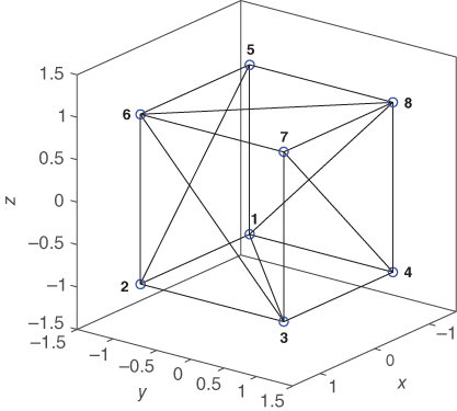
Figure 3.5Formation acquisition: desired formation  .
.
The initial conditions of the agents were randomly selected by

where the function ![]() generates a random
generates a random ![]() vector whose elements are uniformly distributed on the interval
vector whose elements are uniformly distributed on the interval ![]() . Both control gains
. Both control gains ![]() and
and ![]() were set to 1.
were set to 1.
The agent trajectories in space as they converge to the desired cube formation are shown in Figure 3.6. All 28 inter‐agent distance errors ![]() ,
, ![]() are depicted in Figure 3.7, confirming the acquisition of the desired formation. In Figure 3.8 we plot the
are depicted in Figure 3.7, confirming the acquisition of the desired formation. In Figure 3.8 we plot the ![]() ‐,
‐, ![]() ‐, and
‐, and ![]() ‐direction components of the velocity‐related error variable
‐direction components of the velocity‐related error variable ![]() defined in 3.4, which according to Theorem 3.1 should converge to zero. Finally, Figure 3.9 shows the components of the acceleration‐level control inputs.
defined in 3.4, which according to Theorem 3.1 should converge to zero. Finally, Figure 3.9 shows the components of the acceleration‐level control inputs.

Figure 3.6Formation acquisition: agent trajectories  ,
,  .
.

Figure 3.7Formation acquisition: distance errors  ,
,  .
.

Figure 3.8Formation acquisition: velocity errors  ,
,  .
.

Figure 3.9Formation acquisition: control inputs  ,
,  .
.
3.6.2 Dynamic Formation Acquisition with Maneuvering
This simulation combines formation maneuvering with dynamic formation acquisition as discussed at the end of Section 3.5. For this case, the desired dynamic formation ![]() was set to a cube that expanded and contracted uniformly over time. The desired formation was initialized as the cube with edge length of 2 shown in Figure 3.5. The eight vertices of the cube represented the followers while agent 9 at the geometric center of the cube was the leader through which the rotation axis passed. We ensured the desired framework was minimally rigid and infinitesimally rigid by imposing 21 (
was set to a cube that expanded and contracted uniformly over time. The desired formation was initialized as the cube with edge length of 2 shown in Figure 3.5. The eight vertices of the cube represented the followers while agent 9 at the geometric center of the cube was the leader through which the rotation axis passed. We ensured the desired framework was minimally rigid and infinitesimally rigid by imposing 21 (![]() ) edges with all followers connected to the leader. The edge set was selected as
) edges with all followers connected to the leader. The edge set was selected as
The desired formation was made dynamic by setting the vertex coordinates to ![]() where
where ![]() was defined in (2.81). The maneuvering velocity
was defined in (2.81). The maneuvering velocity ![]() in (2.24) was set to have the following translational and rotational components
in (2.24) was set to have the following translational and rotational components
which results in a screw‐like motion for the formation. Control gains ![]() and
and ![]() were again set to 1, while initial conditions were chosen according to 3.28.
were again set to 1, while initial conditions were chosen according to 3.28.
Snapshots in time of the actual formation are shown in Figure 3.10, where the dotted line marks the trajectory of the leader. The 36 inter‐agent distance errors are given in Figure 3.11, while the velocity errors are shown in Figure 3.12. In Figure 3.13, the control inputs are depicted.

Figure 3.10Dynamic formation acquisition with maneuvering: snapshots of  at different instants of time.

Figure 3.11Dynamic formation acquisition with maneuvering: distance errors  ,
,  .
.
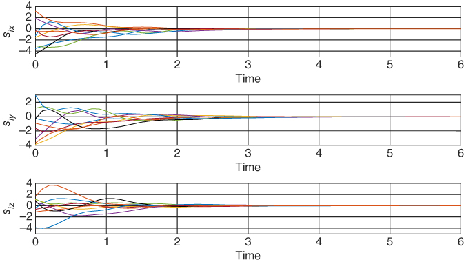
Figure 3.12Dynamic formation acquisition with maneuvering: velocity errors  ,
,  .
.

Figure 3.13Dynamic formation acquisition with maneuvering: control inputs  ,
,  .
.
3.6.3 Target Interception
In this simulation, the desired formation ![]() was set to the framework in Figure 3.5 with edge set 3.29. The leader, who is responsible for tracking the target, was agent 9. The velocity of the moving target was chosen as
was set to the framework in Figure 3.5 with edge set 3.29. The leader, who is responsible for tracking the target, was agent 9. The velocity of the moving target was chosen as
with initial position ![]() . The initial conditions of the agents were chosen according to 3.28, while the control gains in 3.19–3.21 were set to
. The initial conditions of the agents were chosen according to 3.28, while the control gains in 3.19–3.21 were set to ![]() ,
, ![]() ,
, ![]() , and
, and ![]() .
.
Figure 3.14 shows the leader intercepting the target while the followers simultaneously surround it with the cube formation. All 36 inter‐agent distance errors are given in Figure 3.15 with the left (resp., right) plots showing the transient (resp., steady‐state) behavior. The directional components of the velocity errors and control inputs of each agent are shown in Figures 3.16 and 3.17, respectively. Note that the chattering‐like appearance of the control inputs stems from the discontinuous term sgn![]() in 3.19.
in 3.19.

Figure 3.14Target interception: snapshots of  at different instants of time along with target motion.

Figure 3.15Target interception: distance errors  ,
,  .
.

Figure 3.16Target interception: velocity errors  ,
,  .
.

Figure 3.17Figure 3.17Target interception: control inputs  ,
,  .
.
3.7 Notes and References
Formation controllers based on the double‐integrator model are not as prevalent as single‐integrator‐based ones, especially within the realm of inter‐agent distance control. As in Chapter 2, the discussion below is mostly focused on results that explicitly or implicitly address the formation control problem.
In 34,48, the double‐integrator, inter‐agent distance dynamics for formation acquisition were described as a Hamiltonian system and the local asymptotic stability of undirected formations was achieved under a gradient‐like control law. In 46, the gradient formation acquisition law was extended to the double‐integrator model for tree formation graphs. Formation acquisition and flocking control systems were studied in 78 where the invariant properties between single‐ and double‐integrator formation systems were established by employing a parameterized Hamiltonian system.
A dynamic formation maneuvering control law was presented in 79 that decouples formation acquisition from maneuvering using virtual bodies and artificial repel‐attract potentials. Decoupling was achieved by parameterizing the virtual body motion by the scalar variable whose speed and direction can be prescribed. Recall that the general idea of decoupling formation acquisition and maneuvering was also used in the control designs of Sections 2.2 and 3.3 by exploiting the structure of the rigidity matrix (see (1.20)).
In 80, the time‐varying formation problem, which includes formation maneuvering and dynamic formation, was transformed into a consensus problem with respect to a formation center function. A 2D formation maneuvering controller was proposed in 81 where the group leader, who has inertial frame information, passes the information to other agents through a directed path in the graph. A limitation of this control is that it becomes unbounded if the desired formation maneuvering velocity is zero. A synchronization strategy was applied to the formation maneuvering problem in 82 where agents track their individual desired trajectory while synchronizing their relative motions to maintain the desired formation. A consensus scheme was presented in 83 using both the single‐ and double‐integrator models where the formation translation velocity is constant and known to only two leader agents. In 84, existing gradient controllers were modified to ensure finite time formation acquisition and flocking. A similar problem was addressed in 85 but with asymptotic formation acquisition and velocity consensus.
The consensus‐type algorithms for formation control proposed in 39 were extended by the authors to the double‐integrator dynamics. Several problems were discussed, including consensus conditions for fixed and switching interaction graphs, bounded control effort, and elimination of agent velocity measurements.
The interesting problem of containment control was studied in 86, where the followers move in the convex hull spanned by multiple leaders while the leaders perform formation maneuvers. Experiments using wheeled mobile robots were provided to validate the containment algorithms.
The first use of backstepping to deal with the double‐integrator model appeared in 87. The goal of this work was to extend the single‐integrator result of 65 (formation acquisition for three agents with directed graphs) to the double‐integrator case with formation translation. Comprehensive coverage of the integrator backstepping control technique can be found in 9.
The work in 88 considered the problem of dynamic formation acquisition with scaling of the formation size, where only a subset of agents know the desired scaling size but all agents know the desired formation shape. Recently, 89 analyzed the influence of mismatches on the measured distances of neighboring agents on the standard gradient‐based rigid formation control for double‐integrator agents. It was shown that, like the single‐integrator case discussed in 58, these mismatches introduce a distorted final shape and a steady‐state motion of the formation.
The material in this chapter is based on the work in 74, 75, 90, 91.