Analysis of covariance (ANCOVA) involves a combination of regression and analysis of variance. The response variable is continuous, and there is at least one continuous explanatory variable and at least one categorical explanatory variable. Typically, the maximal model involves estimating a slope and an intercept (the regression part of the exercise) for each level of the categorical variable(s) (the ANOVA part of the exercise). Let us take a concrete example. Suppose we are modelling weight (the response variable) as a function of sex and age. Sex is a factor with two levels (male and female) and age is a continuous variable. The maximal model therefore has four parameters: two slopes (a slope for males and a slope for females) and two intercepts (one for males and one for females) like this:

Model simplification is an essential part of ANCOVA, because the principle of parsimony requires that we keep as few parameters in the model as possible.

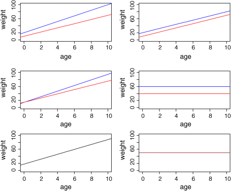
There are at least six possible models in this case, and the process of model simplification begins by asking whether we need all four parameters (top left). Perhaps we could make do with two intercepts and a common slope (top right). Or a common intercept and two different slopes (centre left). There again, age may have no significant effect on the response, so we only need two parameters to describe the main effects of sex on weight; this would show up as two separated, horizontal lines in the plot (one mean weight for each sex; centre right). Alternatively, there may be no effect of sex at all, in which case we only need two parameters (one slope and one intercept) to describe the effect of age on weight (bottom left). In the limit, neither the continuous nor the categorical explanatory variables might have any significant effect on the response, in which case model simplification will lead to the one-parameter null model (a single, horizontal line; bottom right).

Decisions about model simplification are based on the explanatory power of the model: if the simpler model does not explain significantly less of the variation in the response, then the simpler model is preferred. Tests of explanatory power are carried out using anova or AIC to compare two models: when using anova we shall only retain the more complicated model if the p value from comparing the two models is less than 0.05. When using AIC we simply prefer the model with the lower value.

Let us see how this all works by investigating a realistic example. The dataframe concerns an experiment on a plant's ability to regrow and produce seeds following grazing. The initial, pre-grazing size of the plant is recorded as the diameter of the top of its rootstock. Grazing is a two-level factor: grazed or ungrazed (protected by fences). The response is the weight of seeds produced per plant at the end of the growing season. Our expectation is that big plants will produce more seeds than small plants and that grazed plants will produce fewer seeds than ungrazed plants. Let us see what actually happened:

compensation <- read.csv("c:\temp\ipomopsis.csv")
attach(compensation)
names(compensation)

[1] "Root"    "Fruit"   "Grazing"

We begin with data inspection. First: did initial plant size matter?

plot(Root,Fruit,pch=16,col="blue")

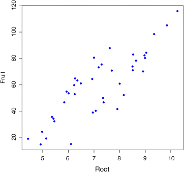
Yes, indeed. Bigger plants produced more seeds at the end of the growing season. What about grazing?

plot(Grazing,Fruit,col="lightgreen")

This is not at all what we expected to see. Apparently, the grazed plants produced more seeds, not less than the ungrazed plants. Taken at face value, the effect looks to be statistically significant (p < 0.03):

summary(aov(Fruit~Grazing))

               Df   Sum Sq  Mean Sq  F value  Pr(>F)  
Grazing          1   2910   2910.4     5.309  0.0268 *
Residuals       38  20833    548.2   

We shall return to this after we have carried out the statistical modelling properly.

Analysis of covariance is done in the familiar way: it is just that the explanatory variables are a mixture of continuous and categorical variables. We start by fitting the most complicated model, with different slopes and intercepts for the grazed and ungrazed plants. For this, we use the asterisk operator:

model <- lm(Fruit~Root*Grazing)

An important thing to realize about analysis of covariance is that order matters. Look at the regression sum of squares in the ANOVA table when we fit root first:

summary.aov(model)
             Df  Sum Sq    Mean Sq   F value   Pr(>F)    
Root          1    16795      16795  359.968  < 2e-16 ***
Grazing       1     5264       5264  112.832 1.21e-12 ***
Root:Grazing  1        5          5     0.103    0.75    
Residuals    36     1680         47    

and when we fit root second:

model <- lm(Fruit~Grazing*Root)
summary.aov(model)

Grazing       1   2910    2910  62.380 2.26e-09 ***
Root          1  19149   19149 410.420  < 2e-16 ***
Grazing:Root  1      5       5   0.103     0.75    
Residuals    36   1680      47  

In both cases, the error sum of squares (1680) and the interaction sum of squares (5) are the same, but the regression sum of squares (labelled Root) is much greater when root is fitted to the model after grazing (19,149), than when it is fitted first (16,795). This is because the data for ANCOVA are typically non-orthogonal. Remember, with non-orthogonal data, order matters (Box 9.1).

Back to the analysis. The interaction, SSR_diff, representing differences in slope between the grazed and ungrazed treatments, appears to be insignificant, so we remove it:

model2 <- lm(Fruit~Grazing+Root)

Notice the use of + rather than * in the model formula. This says ‘fit different intercepts for grazed and ungrazed plants, but fit the same slope to both graphs’. Does this simpler model have significantly lower explanatory power? We use anova to find out:

anova(model,model2)

Analysis of Variance Table

Model   1:   Fruit    ~  Grazing  *  Root
Model   2:   Fruit    ~  Grazing  +  Root
  Res.Df    RSS Df Sum of Sq      F Pr(>F)
1     36 1679.7                           
2     37 1684.5 -1   -4.8122 0.1031   0.75

The simpler model does not have significantly lower explanatory power (p = 0.75), so we adopt it. Note that we did not have to do the anova in this case: the p value given in the summary.aov(model) table gave the correct, deletion p value. Here are the parameter estimates from our minimal adequate model:

summary.lm(model2)

Coefficients:
                Estimate Std. Error t value Pr  (>|t|)    
(Intercept)     -127.829      9.664  -13.23 1.35e-15 ***
GrazingUngrazed   36.103      3.357   10.75 6.11e-13 ***
Root              23.560      1.149   20.51  < 2e-16 ***

Residual standard error: 6.747 on 37 degrees of freedom
Multiple R-squared:  0.9291,    Adjusted R-squared:  0.9252 
F-statistic: 242.3 on 2 and 37 DF,  p-value: < 2.2e-16

The model has high explanatory power, accounting for more than 90% of the variation in seed production (multiple r²). The hard thing about ANCOVA is understanding what the parameter estimates mean. Starting at the top, the first row, as labelled, contains an intercept. It is the intercept for the graph of seed production against initial rootstock size for the grazing treatment whose factor level comes first in the alphabet. To see which one this is, we can use levels:

levels(Grazing)

[1] "Grazed"   "Ungrazed"

So the intercept is for the grazed plants. The second row, labelled GrazingUngrazed, is a difference between two intercepts. To get the intercept for the ungrazed plants, we need to add 36.103 to the intercept for the grazed plants (−127.829 + 36.103 = −91.726). The third row, labelled Root, is a slope: it is the gradient of the graph of seed production against initial rootstock size, and it is the same for both grazed and ungrazed plants. If there had been a significant interaction term, this would have appeared in row 4 as a difference between two slopes.

We can now plot the fitted model through the scatterplot. It will be useful to have different colours for the grazed (red) and ungrazed plants (green)

plot(Root,Fruit,pch=21,bg=(1+as.numeric(Grazing)))

Note the use of 1+as.numeric(Grazing) to produce the different colours: 2 (red) for Grazed and 3 (green) for ungrazed. Let us add a legend to make this clear:

legend(locator(1),c("grazed","ungrazed"),col=c(2,3),pch=16)

Just position the cursor where you want the top left-hand corner of the key to appear, then click:

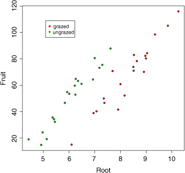
Now it becomes clear why we got the curious result at the beginning, in which grazing appeared to increase seed production. Clearly what has happened is that the majority of big plants ended up in the grazed treatment (red symbols). If you compare like with like (e.g. plants at 7 mm initial root diameter), it is clear that the ungrazed plants (green symbols) produced more seed than the grazed plants (36.103 more, to be precise). This will become clearer when we fit the lines predicted by model2:

abline(-127.829,23.56,col="blue")
abline(-127.829+36.103,23.56,col="blue")

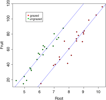
This example shows the great strength of analysis of covariance. By controlling for initial plant size, we have completely reversed the interpretation. The naïve first impression was that grazing increased seed production:

tapply(Fruit,Grazing,mean)

     Grazed      Ungrazed 
   67.9405       50.8805

and this was significant if we were rash enough to fit grazing on its own (p = 0.0268 as we saw earlier). But when we do the correct ANCOVA, we find the opposite result: grazing significantly reduces seed production for plants of comparable initial size; for example from 77.46 to 41.36 at mean rootstock size:

-127.829+36.103+23.56*mean(Root)

[1] 77.4619

-127.829+23.56*mean(Root)

[1] 41.35889

The moral is clear. When you have covariates (like initial size in this example), then use them. This can do no harm, because if the covariates are not significant, they will drop out during model simplification. Also remember that in ANCOVA, order matters. So always start model simplification by removing the highest-order interaction terms first. In ANCOVA, these interaction terms are differences between slopes for different factor levels (recall that in multi-way ANOVA, the interaction terms were differences between means). Other ANCOVAs are described in Chapters 13, 14 and 15 in the context of count data, proportion data and binary response variables.