Chapter 4
Building a Financial Model by the Rulebook
IN THIS CHAPTER
![]() Documenting assumptions
Documenting assumptions
![]() Creating dynamic formulas using links
Creating dynamic formulas using links
![]() Entering data once
Entering data once
![]() Modeling with consistent formulas
Modeling with consistent formulas
![]() Building error checks
Building error checks
![]() Formatting and labeling your models
Formatting and labeling your models
Because Excel is such a wonderfully flexible and universal tool, you can pretty much do anything with it — but that doesn’t mean you should! A key danger of using Excel is lack of discipline, leading to dangerous errors. When building a financial model in Excel, you’re unlikely to encounter the limitations and boundaries imposed by other, less flexible software, so there are certain rules you should follow to avoid these issues. In this chapter, I fill you in on the key rules you should follow when building a financial model.
Document Your Assumptions
The term “garbage in, garbage out” is never truer than in relation to financial modeling. You can have the most beautifully laid-out financial model with perfect formatting, a great design, and fabulous-looking charts and scenario tables, but if the inputs that go into the financial model haven’t been verified, the model is useless and you can’t use the outputs. Important decisions are made based on the outputs of financial models, so listing the assumptions that have gone into the model is critical.
 Documentation of assumptions is certainly not the most exciting part of financial modeling, so you may be tempted to leave it to the end. Don’t fall into this trap! When you’re done building your model, you won’t remember what those assumptions were. Document as you go. Whenever you make a structural change or even a minor change to one of the inputs, document it, even it if it seems unimportant at the time.
 List assumptions on a separate page, and label them clearly, so that they can be easily identified and referenced at a glance. For a small model, you may decide to mix source data and assumptions together. In a large model, you may separate them with as much detail as is possible or practical. For a detailed model, you may list out every single detail on a Detailed Assumptions page and then summarize the important ones on a Key Assumptions page. Think about the level of detail in your model, and let that guide the detail of your documentation of assumptions.
Still not convinced that documenting assumptions is important? How’s this for persuasion: When you move on to another role or you’re away on vacation, and something goes wrong with your model, who do you think they’re going to blame? You guessed it! Think of documenting assumptions as covering your ass. Your model needs to be able to speak for you when you aren’t around to explain or defend your work. The documentation of assumptions should explain your thought process and why the model is built the way it is. That way, if there are any questions as to the accuracy of the model or the input assumptions, they can be easily explained by the model itself.
 A model is only as good as the accuracy of the assumptions. You need to mitigate your liability by documenting your assumptions thoroughly and adding caveats where necessary.
Here are some commonly used methods for including documentation in a model:
-
In-cell comments: There are two different methods of creating in-cell comments:
-
Red triangle comments: The most common method of creating an in-cell comment is to simply insert a comment within the cell, which appears as a red triangle in the corner of the cell, as shown in Figure 4-1.
To create a red triangle comment, right-click the cell and select Insert Comment. To make a change to an existing comment, right-click the cell with the comment and select Edit Comment. Similarly, to delete a comment, right-click the cell and select Delete Comment.
If you want to try the examples out for yourself, you can download File 0401.xlsx at
www.dummies.com/go/financialmodelinginexcelfdand select the tab labeled 4-1. -
Data validation input messages: The less common method of creating an in-cell comment is to use data validations. These types of comments are more discreet, because they don’t have the red triangle in the corner and you don’t see the comment until you actually click on the cell, as shown in Figure 4-2.
This sort of in-cell comment is especially useful for creating little instructions and warnings regarding input data to users, because they won’t see the comment until they actually click the cell to enter the data.
To create a data validation input message, click the cell and then, in the Data Tools section of the Data tab of the Ribbon, click the Data Validation button and the Data Validation dialog box appears. Select the Input Message tab, and type the message you want to appear. This message will appear only when the cell is selected.
Documentation of assumptions using in-cell comments is most appropriate for specific information relating to only one cell or range, because they can be viewed only in a single cell. In-cell comments are useful for communicating details to another modeler about specific calculation details, because the comments are shown only on-screen and won’t show when printed out. More wide-ranging, generic assumptions should be documented using other methods.
Of the two types of in-cell comments, my personal preference is the data validation input message, because they’re neater and cleaner looking. Remember, though, that if the cell isn’t selected, the comment won’t be viewed, so make sure that the comment is only cell-specific. More important, general assumptions and comments should use plain text or another method of documentation.
-
- Hyperlinks: There are two different types of hyperlinks that are useful for documenting assumptions and source data in financial modeling:
-
Cell and file hyperlinks: You can create hyperlinks to sources or other reference files and other sections of a model. Cell and file hyperlinks can aid in navigation of a long and complex model. They’re especially helpful for new users to find their way around the model.
To insert this kind of hyperlink, on the Insert tab, select the Hyperlink icon from the Links section. On the left side, select Place in This Document. Then select the sheet and cell reference or named range of the hyperlink source. You can change the Text to Display at the top to display something like Go to Calculations instead of Calculations!B147, for example. Similarly, you can insert a hyperlink to another file for source referencing.
-
URL hyperlinks: Hyperlinks can also be used to refer to relevant websites directly from your spreadsheet. For example, if the interest rate you assume in your financial model came from a central bank’s website, you can simply copy the URL into a cell in your model. Note that if you’re using Get & Transform (formerly called Power Query) you can link data straight from external data sources, including websites, directly into your spreadsheet, which can be quickly updated without having to manually open the website.
If you’re not using Get & Transform, you can manually insert a URL hyperlink by copying and pasting the URL from the browser directly into the cell. If you don’t want to show a messy URL, you can show different text. On the Insert tab, select the Hyperlink icon from the Links section, and then select Existing File or Web Page. Paste the URL into the Address field at the bottom, and change the Text to Display at the top.
-
- Hard-coded text: This method of assumptions documentation is not very sophisticated, but as with many things in financial modeling, the simple solution is often best. As you can see in Figure 4-3, the assumption has been simply typed into the cell below the calculation table. There is no danger here that a modeler or user might overlook this assumption, whether it’s being viewed on the computer or in a printout.
-
Linked dynamic text: Documenting assumptions liberally within your model is very important, but it’s very difficult to keep the documentation up-to-date when your model is dynamic and inputs are continually changing. For example, in the project costings model shown in Figure 4-4, you want to make sure that the person using the model understands that only 15 hours has been entered into the model, so you want to put the commentary below “Calculations based on 15 hours of billable time spent.” This seems fairly obvious in this example, but if the model were more complex, and the inputs were on a different page, it would be useful to include this comment.
If you were to simply type the text “Calculations based on 15 hours of billable time spent” manually into cell A10, this would be correct … until someone changes the number of billable hours spent on the project, and then the text would quickly become out-of-date. There is a very high risk in this case that you could distribute the model with incorrect assumption documentation.
Instead of typing in the hard-coded value of 15, you can convert the text to a dynamic formula using an ampersand (&), as shown in Figure 4-4. If this formula is used, it will automatically change if the value in C2 changes:
="Calculations based on "&C2&" hours of billable time spent."Download File 0401.xlsx at
www.dummies.com/go/financialmodelinginexcelfdand select the tab labeled 4-4 to try this out for yourself. Change the value 15 in cell C2 to another value, such as 20, and you’ll see that text changes from “Calculations based on 15 hours of billable time spent” to “Calculations based on 20 hours of billable time spent.”

FIGURE 4-1: Red triangle comments.

FIGURE 4-2: Data validation input messages.

FIGURE 4-3: Hard-coded text.

FIGURE 4-4: Linked dynamic text.
Create Dynamic Formulas Using Links
In financial modeling, you need to understand the difference between linked and hard-coded numbers. A linked number will automatically change when the source data changes. In Figure 4-5, cell C3 contains the formula =B3*$C$2. This means that if, say, the number of hours spent on the project in cell C3 changes from 15 to 20, the cost of the team leader will change from $1,200 to $1,600. If you want to try this out for yourself, you can download File 0401.xlsx at www.dummies.com/go/financialmodelinginexcelfd and select the tab labeled 4-5.

FIGURE 4-5: Formulas versus hard-coded numbers.
In comparison, cells C2 and cells B3 to B6 contain hard-coded numbers. These are simply typed directly into the cell and won’t change unless a user manually changes them. These cells can also be called input cells because if a user or modeler changes them, it will change the model output calculations.
Format cells containing hard-coded numbers differently so that it’s obvious to the user which cells can be changed and which cannot. By formatting input cells differently, it’s a signal to your user or another modeler that this is a hard-coded input variable that is designed to change if necessary. Excel has helpfully provided an Input style on the Home tab, as shown in Figure 4-6. There is no hard-and-fast rule that says that you must use this particular format, but it’s important that you do use a consistent format throughout your model so that the user can see at a glance which cells should be changed, and which should not.

FIGURE 4-6: Input style on the Home tab.
This process of linking calculation cells to input cells is an important concept in financial modeling. Always link as much as possible so that when the model inputs change, the outputs also change. The only hard-coding should be input cells. To find out more about linking between cells, sheets, and external files, see Chapter 6.
By linking, you can trace source data back through the links, making your model auditable, traceable, and easy to validate. If you got the input from somewhere, you should document where it came from wherever possible, because that will help with auditing and validation, and give your model credibility.
Only Enter Data Once
When entering data, you should document where it came from if possible, and then link to it with formulas. This may sound obvious but be careful never to enter the same value twice — enter it once as a source and always reference that one cell.
During a long and complex model build, it’s very easy to forget that you’ve entered certain assumptions or inputs, and then enter them again in a different part of the model. For example, in my intermediate online financial modeling course, we build a business case from start to finish, during which we use inflation multiple times within the model, both for indexing salaries, as well as increasing the revenue charged to the customers. Because we’ve entered the inflation in a single cell on the assumptions page, and then referred to it multiple times throughout the model, any fluctuation in the interest rate can be quickly and easily applied throughout the model.
Never type a value within a formula. A calculation such as =453*24 should not appear in a financial model. Similarly, a statement such as =IF(H$6<=$E7,0,157000) should have a link, not 157000 typed in. The only exceptions to this rule are those things that are standard or commonly accepted values that will not change, such as 24 hours in a day, 7 days in a week, or 12 months in a year. In fact, some hard-core modelers even say that you should put the value 12 in a separate cell, and then link to that cell as an assumption that there are 12 months in the year, but I think that’s taking it a bit far!
Try to link directly to the source data where possible. If you link to a link, this creates spaghetti links within your model, which can cause problems later on. To find out more about spaghetti links, turn to Chapter 14.
Model with Consistent Formulas
If you’re getting a model audited by a third party, one of the many things they’ll check for is the number of unique formulas in the model. A good modeler will create as few unique formulas as possible as he’s building a model. In the following example, I’m calculating portfolio returns of different amounts. Figure 4-7 shows the formulas, rather than the calculated values. The way this block has been created in this instance, nine different formulas have been used, which is a very slow and inefficient way of creating this calculation block.

FIGURE 4-7: Calculating portfolio returns using nine unique formulas.
Download File 0401.xlsx at www.dummies.com/go/financialmodelinginexcelfd and select the tab labeled 4-7 or simply open Excel, re-create this example and try it out for yourself. You’ll see that creating the formulas shown in Figure 4-7 is a slow and tedious process.
 If the formulas aren’t all showing when you download and open this file, click the Show Formulas button in the Auditing group on the Formulas tab in the Ribbon. Or, you can use the Ctrl+` shortcut (the ` symbol can be found to the left of the 1 on most keyboards, under the ~ sign).
The task is made much simpler by merely including a few dollar signs in the formula in cell B2 and then copying. Using one single formula and then copying it across and down the calculation block, as shown in Figure 4-8, is much quicker and less prone to error.

FIGURE 4-8: Calculating portfolio returns using one single formula.
Using mixed referencing within the formula — by putting a dollar sign before the row or column to be anchored — is a far more efficient way of modeling. For more information about how to use relative, absolute, and mixed cell referencing, and for step-by-step instructions for completing this example, see Chapter 6.
This concept of building your models with consistent formulas wherever possible saves time, avoids error, and is much easier to audit. And it’s a key component of good financial modeling. If you only pick up one modeling technique from this book, this is it!
Modelers should strive for consistency of formulas within models for all the reasons I outline in this section, but consistency, in general, is something to aim for in all aspects of the model build. Use consistent colors and formatting, consistent labels, and even consistent layouts. If sheets are similar, work on the sheet until you’re completely happy with the layout, and then copy the sheet. This way, the design, formatting, and layout will be identical. Then when you need to update it, group the sheets to make global changes. Have columns and rows matching on multiple sheets — for example, on calculation sheets, if January’s calculations start in column F, then January should always start in column F on every calculation sheet.
Build in Error Checks
Even if you’ve only just started modeling, you’re probably well aware how easy it is to make a mistake in a financial model! There are three ways to prevent errors in a financial model:
- Avoid making the mistakes in the first place. In this book, I describe several techniques that you can employ to avoid making mistakes in the first place, such as being consistent with your formulas.
- Check the model for errors. Despite your best efforts, errors inevitably may slip through, so check, double-check, and have someone else check your model after it’s complete.
- Include error checks. As you’re building the model, include error checks that prevent inadvertent errors from slipping into the model due to incorrect entries or user error.
For more examples of different types of commonly made mistakes, and some ways to avoid making these errors in your models, see Chapter 13. This section focuses on the first two points: techniques for model building to reduce error, as well as ways to check the model for errors.
Error checks are a critical part of a well-built financial model so that the user or modeler can see at a glance if the formulas are calculating correctly. For example, when creating management reports, check that the sum of each individual department’s report adds to the company-wide total. This can be done by inserting a simple IF function, among other methods.
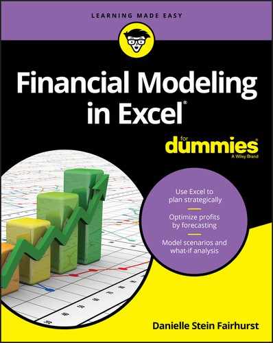
In the example shown in Figure 4-9, a capital budget has been built with estimated spend dates in column E. In the capital spend schedule shown in columns F through Q, the spend gets spread out over the full year. The modeler knows that the total capital spend amount of $124,700 shown in cell D17 should be the same as the total capital schedule amount shown in cell R17, and if the two amounts do not equal each other, then the model is not calculating properly. So the error-checking cell E1 contains the very simple formula =R17-D17.
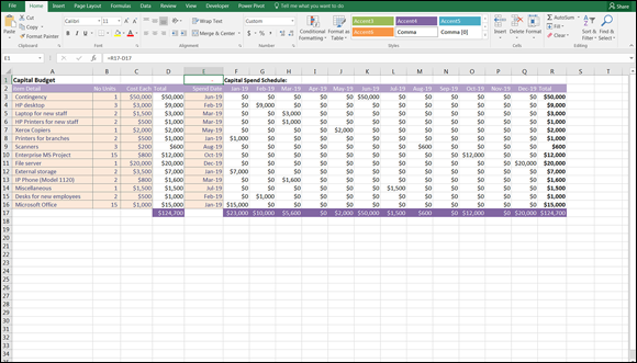
FIGURE 4-9: A simple error check.
In Figure 4-10, you can see that a user has entered an incorrect value in cell E4. Feb-20 is not a valid entry because the capital spend schedule only allows for dates during 2019. This means that the financial model shown in Figure 4-10 is incorrect — the user has entered $124,700 worth of capital expenditure into the model, but only $115,700 has been allocated across the year. The number showing in cell E1 (9,000) alerts the user to the fact that there is a problem. Download File 0401.xlsx at www.dummies.com/go/financialmodelinginexcelfd and select the tabs labeled 4-9 and 4-10 to try triggering this error check for yourself.

FIGURE 4-10: An error check triggered.
This error check is very simple and quite discreet. To make it more obvious, you may prefer to include the description “error check” next to the error checking cell in cell D1, which would make it more obvious to the user what has happened when the error check is triggered.
The error check shown in Figure 4-10 is my preferred method of error checking, because it’s so simple and quick to build. Because it returns a value in the case of an error, it may be a little too discreet for your tastes — it doesn’t necessarily alert the user immediately that an error had been made. However, it’s certainly quick and easy to follow and, for this reason, a fairly common error check favored by many modelers.
If you use this kind of error check, format it using the Comma style (found on the Home tab in the Numbers group) and remove the decimal place and format it with a red font. This way, the zero won’t show if there is no error, and a red number will show if there is an error.
Alternatively, you may prefer the other error checking formula such as =D17=R17, which will return the value TRUE if they are the same or FALSE if they aren’t. However, this method is also subject to a false error, as shown in the following section.
Allowing tolerance for error
=IF(D17<>R17,”error”,0) is a superior error check, but every now and then it can return a false error result, even though the values are the same. (See Chapter 7 for how to use an IF statement in a formula like this.) This “bug” in an error check is caused by the fact that Excel carries calculations to 14 decimal places. After that, it truncates the value and can cause a minute discrepancy, which will report an error when it’s only 0.00000000000001 off. To avoid this potential issue, you could use an absolute value formula, which would allow a tolerance for error. =IF(ABS(D17-R17)>1,”error”,0) will allow the values to be off by $1 before it reports an error. If you use the ABS function in Excel, this will take the absolute value of the result, so it doesn’t matter if it’s a positive or negative number.
There are many variations of this formula. Some modelers prefer to show the word OK if the numbers are right, and Check if they aren’t.
Applying conditional formatting to an error check
To make the error check even more prominent to the user, consider using conditional formatting to add a rule that makes the entire cell turn red if the error check has been triggered. On the Home Tab of the Ribbon, in the Styles group, click the Conditional Formatting button. Then hover the mouse over Highlight Cells Rule and select Equal To (see Figure 4-11).
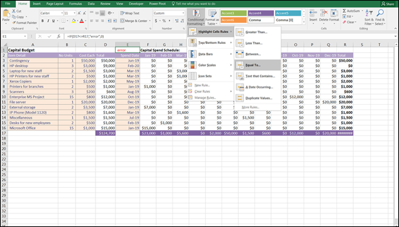
FIGURE 4-11: Applying conditional formatting to an error check.
When the Equal To dialog box appears, as shown in Figure 4-12, type the word error into the Format Cells that are EQUAL TO box and click OK. By default, it will turn the cell to Light Red Fill with Dark Red Text, but you can change this in the drop-down box.

FIGURE 4-12: Editing the conditional formatting color.
Conditional formatting is popular in error checks because it makes the error check stand out more when it has been triggered. And, with any luck, the user will realize that there is an error in the financial model. Conditional formatting is not limited to error checks — it can be useful for other models where you want to draw the user’s attention to abnormalities or highlights in the calculations.
Format and Label for Clarity
Applying appropriate formatting and labeling to financial models is sometimes neglected by even experienced financial modelers. You need to include as many descriptions and instructions as possible within the model to make it absolutely obvious how to use the model and how the calculations work. Don’t assume that someone using the model will be able to understand what he’s supposed to do with the model, its purpose, and what should be changed when.
Here are some simple formatting rules to follow:
-
Format input cells differently from calculation cells. (See “Create Dynamic Formulas Using Links,” earlier in this chapter.)
- Use the correct symbols for currency. If the currency is dollars, format 5000 as $5,000 for example, or if it’s in euros, format it as €5,000.
- Use commas for thousands. This makes your model easier to read and prevents mistakes and misinterpretations.
- Include a dedicated units column. Make sure the units denoted by the amounts in that column are entered into that column’s heading (for example, “MWh,” “Liters,” or “Headcount”).
- Label your data clearly. It sounds simple, but mixing units (for example, mixing apples and oranges, or miles and kilometers) is a common source of error in financial modeling, and good formatting and labeling will avoid this.
- If you round figures into thousands, show this clearly at the top of the row with a descriptive heading. For example, make the column heading “Revenue $’000” to avoid confusion and misinterpretation.
- Include units or currencies in column and row headings. Where possible, each column or row should contain only one type of unit or currency.
- Reserve a column for constants that apply to all years, months, or days. For example, if growth rate is 5 percent, have that in column D, and then link all calculations to column D.