Chapter 6
Excel Tools and Techniques for Financial Modeling
IN THIS CHAPTER
![]() Introducing cell referencing
Introducing cell referencing
![]() Applying named ranges
Applying named ranges
![]() Dealing with links and the potential errors they can cause
Dealing with links and the potential errors they can cause
![]() Improving your modeling skills with shortcuts
Improving your modeling skills with shortcuts
![]() Restricting user entry with data validations
Restricting user entry with data validations
![]() Working out a break-even point with goal seek
Working out a break-even point with goal seek
When you’re using Excel for the purpose of financial modeling, much of the emphasis is on selecting the right function to include in the formulas to calculate the results of the model. Besides functions, a number of tools and techniques are also useful to include in your models. Chapter 7 focuses on Excel formulas. This chapter looks at some of the other practical tools and techniques commonly used in financial modeling in Excel.
Referencing Cells
In Chapter 3, I explain why not every spreadsheet built in Excel is a financial model. In order to be able to call your spreadsheet a financial model, it must contain formulas. And in order to build formulas, you need to reference cells. It follows therefore that as a financial modeler, you must understand how to reference cells in Excel.
An Excel worksheet is made up of over a million rows and more than 16,000 columns. Each of these cells is referred to like the coordinates of a map, and the cell references are what you use to build the formula. For example, in Figure 6-1, the cost of $450 has been entered in cell B2. So, if you want to use that value in another cell, you would use the cell reference =B2.

FIGURE 6-1: Cell referencing.
 You can download File 0601.xlsx at
 www.dummies.com/go/financialmodelinginexcelfd.
This kind of reference is called a relative cell reference, and it’s the default way that Excel treats the reference when you first link to a cell. There are three types of cell references, however, and the way you choose to reference a cell will depend on how you want your formula to change when you copy it to other cells:
- Relative cell reference: Both the column letter and the row number change relative to where the formula is copied. A relative cell reference is simply a cell name, such as B2.
- Absolute cell reference: The column letter and row number of a cell name are preceded by dollar signs, such as $B$2, to indicate that the cell reference should not change when copied.
- Mixed cell reference: Either the column letter or row number is preceded by a dollar sign to indicate which of these is to remain unchanged when copied. Both $B2 and B$2 are examples of mixed cell references.
Understanding the difference between relative, absolute, and mixed cell referencing is important when it comes to efficiently building your financial models and maintaining formula consistency. Formula consistency is critical for best practice in financial modeling (and in any other sort of analysis using Excel). In order to have consistent formulas across and down the block of data, you need to understand how cell referencing works. Although cell referencing is a very basic feature of Excel that is taught in introductory Excel courses, it’s surprising how many modelers don’t recognize its importance.
 The dollar sign in cell referencing tells Excel how to treat your references when you copy the cell. If there is a dollar sign in front of a row number or column letter, the row or column does not change when you copy it. Otherwise, it does change. So an absolute reference will not change its cell reference when you copy it, whereas a relative reference will.
I walk you through each of these types of cell referencing in greater detail in the following sections.
Relative cell referencing
Relative cell referencing is the default in Excel. For example, Figure 6-2 calculates the total price by referring to values in cells B2 and A3. The asterisk is used to multiply the numbers in the two cells.

FIGURE 6-2: Relative cell referencing.
Although you can manually type out a cell reference, this may introduce hard-to-detect typing errors. To avoid this problem, enter your cell reference by typing the formula up to the point of the cell reference and then select the cell with the value to be used in your formula. You can do this by clicking the cell with your mouse or using the arrow keys on your keyboard. When you select a cell, Excel automatically places the cell name in your formula.
When you copy a formula with relative references to the cell below, the row number of the references adjust accordingly. In the same way, when you copy the formula to the next cell over, the column letters changes. For example, when the formula in cell B3 is copied down the range, the references automatically change, as shown in Figure 6-3, and the results will be wrong!

FIGURE 6-3: A relative reference copied down (incorrect and not recommended).
To get the correct result using relative references, you’d need to re-create the formula five times instead of copying it down, as shown in Figure 6-4.

FIGURE 6-4: A relative reference built separately (mathematically correct but not recommended).
Although this does give the correct results, it’s not the fastest and easiest way of building this formula. There are several reasons why this solution is not recommended:
- It takes a lot longer to build.
- The formula is prone to error because you’re far more likely to accidentally pick up the wrong cell.
- Updating it will mean having to update each and every formula in the range.
- It’s more difficult for someone else to follow and, hence, more difficult to audit.
Absolute cell referencing
A much better solution would be to use the formula =$B$2*A3 and then copy the formula down the range, as shown in Figure 6-5. Putting one dollar sign before the column letter and another before the row number in the cell reference anchors the reference when it’s copied. This is called an absolute reference.
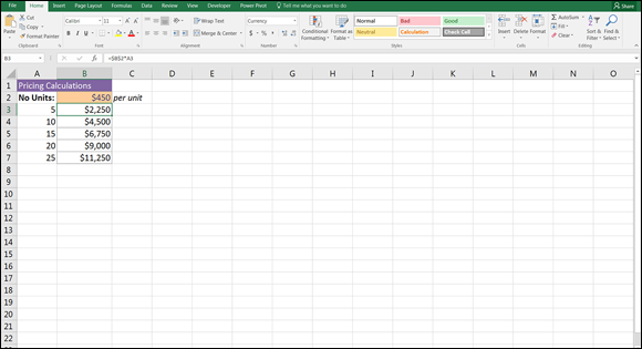
FIGURE 6-5: An absolute reference copied down (recommended).
In this example, the $B$2 part of the formula is an absolute reference, and the A3 part of the formula is a relative reference. As shown in Figure 6-5, the absolute reference remains constant, but the relative reference changes when it’s copied down.
Let’s take a look at a practical example and apply relative and absolute cell referencing to a very simple financial model. You’ve been given the annual salaries for staff members who will work on a particular project. Assume that each person works 260 days in the year, and each person must work 60 days on this project. Calculate the total staff cost of the project.
Download File 0601.xlsx at www.dummies.com/go/financialmodelinginexcelfd and select the tab labeled 6-6, or open a blank workbook and enter and format the data as shown in Figure 6-6. Then follow these steps:
-
In cell C6, enter the formula =B6/B3.
This formula calculates the daily rate of each person by dividing his annual salary by the number of days he works per year. The formula result is $923.08.
-
Press F4 to apply absolute referencing.
The formula changes to =B6/$B$3.
-
Copy this formula down the column.
Now you need to calculate what those project costs are based on the daily rate by multiplying the number of project days by the daily rate.
- In cell D6, enter the formula =D3*C6.
-
When you copy it down, you want the project days reference to remain constant, so press F4 to fix this reference.
The formula is =$D$3*C6 with the resulting value of $55,385.
- Copy this formula down the column.
-
In cell D10, enter the formula =SUM(D6:D9).
The result $146,769, which is the total project cost.
-
Compare your results to Figure 6-7.
You can perform some sensitivity analysis by changing the number of project days in cell D3 from 60 to 65. Change the cost for the business analyst in cell B7 from $120,000 to $150,000. Observe the effect it has on the project costs.

FIGURE 6-6: Calculating daily staff rate using absolute referencing.

FIGURE 6-7: Completed project costs.
Mixed cell referencing
Mixed cell referencing is a combination of relative and absolute referencing; one part of the reference is absolute, and the other is relative. When you add a dollar sign before the row, the row remains anchored when the cell is copied; when you add a dollar sign before the column, the column remains anchored when the cell is copied.
For example, if you create the reference =B2 in a cell, and then copy that reference down, it will change to B3. If you add some anchoring, here are the results in each case:
|
Cell |
Copies as Cell |
|
=B2 |
=B3 |
|
=$B$2 |
=$B$2 |
|
=B$2 |
=B$2 |
|
=$B2 |
=$B3 |
The dollar sign anchors a row number or column letter when you copy it. You can anchor both the column and the row (absolute referencing), or you can anchor one or the other (mixed referencing).
Mixed cell referencing is a concept critical to good financial modeling practice, so it’s important for a financial modeler to understand this fundamental concept. Used effectively, mixed cell references make your model
- Faster to build and more efficient
- Less prone to error
- Quicker, easier, and cheaper to audit
The easiest way to quickly add absolute and mixed cell referencing is to press F4 immediately after adding the reference to the formula. This keyboard shortcut cycles through combinations of relative and absolute referencing. You can repeatedly press F4 after entering the cell name in a formula to cycle through the mixed references. For example, type =B2 and then press F4 to display =$B$2. Press F4 again to display =B$2. Press F4 again to display =$B2. And press F4 again to display =B2.
Let’s look at a practical example of how to use mixed cell referencing. In the following example, you want to calculate how much you’d receive in interest under three different portfolio amounts and three different interest rates. The most efficient way to perform this calculation is to create a single formula with appropriate references and then copy that formula to other cells. You need to create a formula that multiplies the interest amount in row 1 and the borrowing amount in column A.
Instead of creating nine different formulas, you’re creating only one single formula using mixed cell referencing, which you can then copy across, saving you time and reducing the possibility of error.
Follow these steps:
- Download File 0601.xlsx from
www.dummies.com/go/financialmodelinginexcelfdand select the tab labeled 6-8 or create a blank workbook and enter and format the data as shown in Figure 6-8. - In cell B2, type = and then select cell A2 by clicking it or pressing the arrow key.
- Press F4 three times to display the mixed reference $A2.
-
Type *, select cell B1, and this time press F4 twice to display the mixed reference B$1.
To anchor the row, put the dollar sign before the row. To anchor the column, put the dollar sign before the column. -
Press Enter to show the formula =$A2*B$1 in cell B2.
The result is $18,750 as shown in Figure 6-8.
-
Select cell B2 and copy it across and down the rest of the block of data.
Copying and pasting can be done in a several different ways. Choose the option that suits you best:
- Go to the lower-right corner of cell B2 and select the fill handle with the mouse. Drag it across to cell D2 and release the mouse. Then drag down to row 4.
- Copy cell B2 with the shortcut Ctrl+C, and select the entire block either with the mouse or by holding down the Shift key together with the right arrow and down arrow. Press Enter to paste.
- Highlight the entire block of data either with the mouse or by holding down the Shift key together with the right arrow and down arrow. Use the shortcuts Ctrl+R and Ctrl+D to copy right and copy down.
-
Review the results.
Note how your carefully crafted formula generates data for the entire block of cells. Compare your worksheet to the one shown in Figure 6-8.

FIGURE 6-8: Mixed cell referencing.
Maintaining consistency of formulas is a fundamental technique of financial modeling that will save you and anyone else using your model a lot of unnecessary time in building, checking, and auditing the calculations.
When formulas make calculations based on data stored in your spreadsheet, use cell references wherever possible, instead of typing the actual data. Typing numbers into formulas is called hard coding, and it should be avoided unless the numbers are source data — and, if so, documented as such. This rule is also important to follow when building your model because it makes your models much easier to update, both for you and others using your model. If you’ve used cell references instead of hard-coded the numbers into the formula, and you change a value in a cell referenced by a formula, the formula automatically recalculates.
Naming Ranges
Many financial modelers like to include named ranges in their models. Named ranges are just a way of naming a cell, or a range of cells, to use it in a formula, instead of using cell references.
In Figure 6-5 earlier in this chapter, I used an absolute reference to anchor the formula to the consistent price of $450. This cell is called B2, and it won’t change. However, I can also change the name of it to something else, such as “price.” That’s what a named range is.
Understanding why you may want to use a named range
You don’t have to include named ranges in a financial model, and some of the best financial models don’t use them at all. Those who haven’t used them before sometimes struggle to see the benefits of including them in financial models. Most of the time, named ranges aren’t really necessary, but there are a few reasons why you should consider using them in a financial model:
- Named ranges can make your formulas easier to follow. A formula containing lots of cell references can be confusing to look at and difficult to edit. But if the cell references are replaced by a range name, it becomes much easier to understand. For example, the formula =SUM(B3:B24)-SUM(F3:F13) could be expressed as =SUM(Revenue)-SUM(Expenses) to calculate profit.
- Named ranges don’t need absolute referencing. By default, a named range is an absolute reference, so you don’t need to add any in.
- Using named ranges is ideal when you’re linking to external files. When the cell reference in the source file changes (such as when someone inserts a row), the formula linking to it will automatically update, even if the file is closed when the update is made.
- If you decide to use macros in your model, you should use named ranges when referring to cell references in the Visual Basic code. As with external links, this practice is more robust than using cell references.
In general, named ranges just make your life easier as a modeler. They make your formulas neat and tidy, easier to read and follow. You aren’t required to use named ranges in your model, but you should know what they are and how to edit them if you come across named ranges in someone else’s model.
Creating a named range
To create a named range, follow these steps:
- Select cell B2.
-
In the Name box in the upper-left corner (see Figure 6-9), type over the name and call it something else, like Price.
Note that the name you type must not contain any spaces or special characters. For instance, if you want to call it “Year 1 Price,” you need to name it “Year1Price” or “Year1_Price” or something along those lines.
- Press Enter.

FIGURE 6-9: The Name box.
Named ranges don’t necessarily need to be confined to a single cell; you can also create named ranges for an entire range of cells, and these can be used in formulas. Simply highlight the range instead of a single cell, and type over the name.
Finding and using named ranges
Clicking the drop-down arrow next to the Name box shows all the defined names in the workbook, as shown in Figure 6-10.

FIGURE 6-10: Finding a named range using the Name box.
Clicking the name in the drop-down box will take you directly to select that cell or range of cells included in the named range automatically. It doesn’t matter what sheet you’re in when you select the name. This can make finding your way around the named ranges in a model much faster. You can also press Ctrl+G to bring up a dialog box with all the names, or press F3 to paste names.
After you’ve created a range name, you can use that name in a formula instead of cell references. In the example shown in Figure 6-11, you can create the named range Price for cell B2 and the named range Units for the range A3:A7. In cell B3, you can use the formula =Price*Units to calculate the price, and then copy it down the column, as shown in Figure 6-11.

FIGURE 6-11: Using named ranges in a formula.
You can use a named range in a formula in several different ways:
- Simply type =price in a cell.
- Type = and then select cell B2 with the mouse to pick up the name of the cell.
- Press F3 and then double-click the name to paste it into a cell.
- Select the Formulas tab on the Ribbon and, in the Defined Names section, select the name you want to use from the Use in Formula drop-down list.
If you’re planning to use named ranges in your model, create them first, before you build your formulas. Otherwise, you’ll need to go back and rebuild your formulas to include the named ranges.
A cell does not need to be an input field in order to assign a name to it, although it often is in financial models. The cell can also contain a formula as well as a hard-coded input value.
 Named ranges can be useful, but you don’t want to have too many. They can be confusing, especially if you haven’t been consistent in your naming methodology. It’s also quite easy to accidentally name the same cell twice. So in order to keep names neat and tidy, be sure to use the Name Manager to edit or delete any named ranges that are no longer being used. Note that copying sheets into a model can copy named ranges, which can also contain errors as well as external links you’re not aware of. This can slow down the file, so it’s a good idea to look through the Name Manager every now and then to tidy it up.
Editing or deleting a named range
You can manage all the named ranges you’ve created in the Name Manager, which can be found in the Defined Names section on the Formulas tab on the Ribbon. It’s easy to create a named range and forget it’s there, so try to keep your names tidy. If you need to remove a named range or find that you’ve accidentally named the wrong cell, you can add, edit, or delete existing named ranges in the Name Manager.
Linking in Excel
As discussed in Chapter 1, the definition of financial modeling is that when the inputs change, the outputs change as well. Linking in Excel is what makes this happen. If you’re just typing numbers into formulas, such as =453*12, that’s not financial modeling. You need to create a formula that links to a cell or cells so that when the cell changes, the result of your formula will change as well.
There are two types of links in Excel: internal links (links within the model) and external links (links to other files). So far, in this chapter, I’ve been performing links on the same page. Almost every financial model involves multiple pages, though, so it’s almost always necessary to link to other sheets within the same file.
Internal links
In this section, you have some simple profit-and-loss calculations, and you’re going to create a summary report by linking between sheets. Follow these steps:
-
Download File 0602.xlsx from
www.dummies.com/go/financialmodelinginexcelfdand select the tab labeled IS.A completed version is also available in File 0603.xlsx, which you can download and use to compare your work.
-
On the IS worksheet, select the cell C4 and calculate the sales revenue by entering the formula =F3*F4.
The calculated result is $29,502.
-
Go to cell C19 and calculate the manufacturing cost by entering the formula =F19*F3.
The calculated result is $7,152.
-
Go to cell C20 and calculate the sales commission by entering the formula =F20*C4.
The calculated result is $1,475.
-
Excel will sometimes put additional decimal places automatically, so change the number formatting to currency with no decimal places if necessary.
You can do this by pressing the Decrease Decimal icon in the Number section of the Home tab of the Ribbon.
-
Check that the profit margin is calculating correctly.
The calculated result in cell C25 is 20%.
-
Compare your results to Figure 6-12.
Now you have your detailed P&L and you can create a summary on the first worksheet (Summary) using links.
- On the Summary worksheet, select cell B5.
-
Link through the fixed costs by entering the formula =‘IS’!C15.
Do not type this out. Instead, click cell B5, type =, and select the next tab using the mouse. Click cell C15 on the IS tab using the mouse, and press Enter.
- Similarly, select cell B6 on the Summary worksheet and link through the variable costs by adding the formula =‘IS’!C21.
- Go to cell B4, and link through the sales revenue by adding the formula =‘IS’!C4.
-
Compare your results to Figure 6-13.
A good layout for a financial model is to have assumptions together on a single page, usually at the back. Let’s move the assumptions to a separate sheet at the back of the model. Don’t worry — this is a lot easier than it sounds!
- Insert a new sheet by clicking the plus sign behind the last tab.
- Double-click the tab name, and change Sheet1 to Assumptions.
- Go back to the IS worksheet and highlight the area of the sheet that contains the assumptions (cells F1:G20).
- Press Ctrl+X to cut the data onto the clipboard.
-
Go to the Assumptions worksheet, select cell A1, and press Ctrl+V or press Enter to paste the data to the new sheet.
When you have data on the Clipboard, pressing Enter will paste the data and remove it from the Clipboard. Pressing Ctrl+V will leave the data on the Clipboard in case you want to paste it again. Either technique will work in this case. The formulas in this model work in exactly the same way as they did before we moved the assumptions to the new sheet. It’s important that you used cut and paste here, not copy and paste, or the links would not have worked properly. - Go back to the Assumptions worksheet and tidy it up. Remove the blank rows 5 through 18 by highlighting the rows, right-clicking, and pressing Delete.

FIGURE 6-12: The completed income statement.

FIGURE 6-13: The completed income statement summary.
Now you have a simple but tidy model. It links, it’s clear, it’s straightforward, and it’s easy for someone else to understand.
External links
So far, I’ve only been looking at creating links from one cell to another, either on the same sheet or on a different sheet within the same file. Sometimes, however, the data you want to link to exists in another file, so you need to link from one file to another. These are called external links. They’re created in a very similar way to internal links; simply type = and then select the cell in the file you want to link to, and press Enter. Working with external links isn’t as straightforward as working with internal links, however, so it does require a lot more care.
External links can be the cause of many problems, such as broken links, incorrect data, and error messages. Your model will be much simpler if you can avoid external links, but if you decide to include them, you should do so with caution. Most problems happen when users
- Change filenames or move the file to another location.
- Change the source file sheet name when the file linking to it is closed.
- Insert rows or columns in the source file when the file linking to it is closed.
- Email files that contain links.
Improving external links with named ranges
One of the main issues with linking to external files is that if users insert or delete rows or columns in the source file, or change tab names, this causes errors in the files that are linking to it. If you’re lucky, it will show a #REF! error, which you can easily find and correct. If you’re not so lucky, it will show a value that looks as though it is correct, but is in fact completely wrong.
Imagine that you want to use an interest rate in your financial model, which is being generated in another model. This interest rate frequently changes, so you decide to create a link, rather than hard-coding the number. This will save you time having to update it every time. You create a link from your financial model to another source file, using the following link:
=‘C:Plum SolutionsClientsTransactionsFiles[Interest Calculations.xlsx]Sept’!$D$23
If both files are open at the same time, and you insert a row in the Interest Calculations.xlsx file, the link will automatically update from $D$23 to $D$24. However, if your file is closed, your model will not update. This means that the next time you open it, your model will be picking up the wrong cell!
The way around this issue is to create a named range in the source file (for example, the word interest), and then if that cell moves in the source file, the cell will still retain its name, and the formula in your model will still be correct. See the section on “Creating a named range” earlier in this chapter for how to do this:
=‘C:Plum SolutionsClientsTransactionsFiles[Interest Calculations.xlsx]Sept’!interest)
The next time your model tries to update the link, it will look for the name interest, rather than $D$23, and the integrity of the link will be maintained. This is why using named ranges when dealing with external links is considered best practice: It’s a much more robust way of linking files together.
Don’t use formulas in external links. When linking to an external file, use a simple, direct formula such as =‘C:WorkPlum SolutionsClientsTransactionsFilesInterest Calculations.xlsx’!interest. Using more complex formulas, such as SUMIF, can mean that the links show errors unless the files are both open at the same time.
Finding and editing external links
In the Connections group on the Data tab, click Edit Links. The Edit Links dialog box, shown in Figure 6-14, appears. Click the Change Source button to tell your model the new location of the file it has been linked to.

FIGURE 6-14: The Edit Links dialog box.
Another handy use for Edit Links is to break all links in a file. If you’re emailing a file, it isn’t recommended that you leave links in it. You could paste the cell values one by one, but breaking links will convert every single formula in the entire file to their hard-coded values. Click Edit Links, and you’ll be able to select the external files and click the Break Links button.
Sometimes your model will have links that simply won’t break! These “phantom links” are most commonly the result of links contained in named ranges. Deleting the names that contain external links from the Name Manager will remove them from your file. If that doesn’t work, other possible reasons could be links in conditional formatting, charts, objects, or PivotTables.
Using Shortcuts
If you’re spending a lot of time modeling in Excel, you can save yourself a lot of time by learning some keyboard shortcuts. For example, when copying and pasting a cell, you could follow this process:
- Select the cell.
- Right-click with the mouse.
- Select Copy from the contextual menu.
- Highlight the destination range with the mouse.
- Right-click again with the mouse.
- Select Paste from the contextual menu.
Alternatively, you could accomplish the same task using shortcuts:
- Select the cell.
- Press Ctrl+C.
- Use the Shift and arrow keys to move to the destination cells.
- Press Enter (which clears the clipboard) or press Ctrl+V (which leaves what you have copied on the clipboard).
Open Excel and try this for yourself. The second method is a lot quicker, especially with a little practice.
Hundreds of shortcuts are available in Excel. Table 6-1 lists those that are covered in this book and that you should, at a minimum, know. As you continue your journey as a modeler, you’ll no doubt add many more shortcuts to your repertoire.
TABLE 6-1 Excel Shortcuts
|
Shortcut |
Action |
|
Editing | |
|
Ctrl+S |
Save workbook |
|
Ctrl+C |
Copy |
|
Ctrl+V |
Paste |
|
Ctrl+X |
Cut |
|
Ctrl+Z |
Undo |
|
Ctrl+Y |
Redo |
|
Ctrl+A |
Select all |
|
Ctrl+R |
Copies the far left cell across the range (after you highlight the range) |
|
Ctrl+D |
Copies the top cell down the range (after you highlight the range) |
|
Ctrl+B |
Bold |
|
Ctrl+1 |
Format box |
|
Alt+Tab |
Switch program |
|
Alt+F4 |
Close program |
|
Ctrl+N |
New workbook |
|
Shift+F11 |
New worksheet |
|
Ctrl+W |
Close worksheet |
|
Alt+E+L |
Delete a sheet |
|
Ctrl+Tab |
Switch workbooks |
|
Navigating | |
|
Shift+Spacebar |
Highlight row |
|
Ctrl+Spacebar |
Highlight column |
|
Ctrl+– (minus sign) |
Delete selected cells (note that the Del key only clears cells, it does not delete them) |
|
Arrow keys |
Move to new cells |
|
Ctrl+Pg Up/Pg Down |
Switch worksheets |
|
Ctrl+Arrow |
Go to end of continuous range and select a cell |
|
Shift+Arrow |
Select range |
|
Shift+Ctrl+Arrow |
Select continuous range |
|
Home |
Move to beginning of line |
|
Ctrl+Home |
Move to cell A1 |
|
In Formulas | |
|
F2 |
Edit formula, showing precedent cells |
|
Alt+Enter |
Start new line in same cell |
|
Shift+Arrow |
Highlight within cells |
|
F4 |
Change absolute referencing ($) |
|
Esc |
Cancel a cell entry |
|
Alt+= |
Sum selected cells |
|
F9 |
Recalculate all workbooks |
|
Ctrl+[ |
Highlight precedent cells |
|
Ctrl+] |
Highlight dependent cells |
|
F5+Enter |
Go back to original cell |
To find the shortcut for any function, press the Alt key, and the shortcut keys will show on the Ribbon, as shown in Figure 6-15. For example, Remove Duplicates can be performed by selecting the range, and then pressing Alt+A+M.

FIGURE 6-15: Shortcut keys are shown after pressing the Alt key.
In the upper-left corner, you can see the Quick Access Toolbar. You can change the shortcuts that appear here by clicking the tiny arrow to the right of the Quick Access Toolbar and selecting what you want to add from the drop-down box that appears. In Figure 6-15, Paste Special is in the fourth position, so Paste Special can be accessed with the shortcut Alt+4. Note that this only works when you’ve customized the Quick Access Toolbar; whatever you put in the fourth position will be accessed by the shortcut Alt+4.
Restricting and Validating Data
After you finish building a financial model, you may be tempted to keep it to yourself, because you don’t want anyone to mess up your formulas or use the model inappropriately. Models should be collaborative, but you need to build your model in such a way that it’s easy for others to use and difficult to mess up. One great way of making your model robust for others to use is to apply data validations and protections to the model. This way, the user can only enter the data he’s supposed to.
Restricting user data entry
For a practical example of how to use data validation, let’s take the Project Costings Analysis from the “Absolute cell referencing” section earlier in this chapter (refer to Figure 6-6). Your colleague is using the model you’ve built and he can tell by the way in which cell D3 has been formatted (with shading) that you expected people to make changes to it. He’s not sure anymore how many days this project is going to continue, so he types TBA into cell D3 instead. As soon as he types TBA, that really messes things up! As you can see in Figure 6-16, the formulas you’ve already built were expecting a number in cell D3, not text.

FIGURE 6-16: Text in an input causing errors.
Instead of allowing the user to put anything into any cell, you can change the properties of this cell to allow only numbers to be entered. You can also change it to allow only whole numbers or numbers in a given range.
Follow these steps:
- Download File 0601.xlsx from
www.dummies.com/go/financialmodelinginexcelfdand select the tab labeled 6-17. - Select cell D3.
-
Go to the Data tab on the Ribbon and press the Data Validation icon in the Data Tools section (see Figure 6-17).
The Data Validation dialog box appears (refer to Figure 6-17).
- On the Settings tab, in the Allow drop-down list, select Whole Number; in the Data drop-down list, select Greater Than; and in the Minimum field, enter 0.

FIGURE 6-17: Using data validation to restrict entry into cells.
Now only allow whole numbers greater than zero can be entered into cell D3. Try entering text such as TBA. Try entering a negative value. Excel won’t allow it, and an error alert will appear.
If you want, you can enter a warning message on the Input Message tab of the Data Validation dialog box. For example, you might want the following message to appear: “Warning! Only enter numerical values.” On the Error Alert tab, you can enter another message that appears if someone ignores the warning and tries to enter invalid text. I’m usually tempted to type something mischievous, such as: “Invalid entry. Your hard drive will now be completely erased.”
Creating drop-down boxes with data validations
Not only does the data validation tool stop users from entering incorrect data into your model, but you can also use it to create drop-down boxes. In the Data Validation dialog box, from the Allow drop-down list, select List, as shown in Figure 6-18. In the Source field, enter the values you’d like to appear in the list with a comma between them such as Yes, No. A simple drop-down list is created in cell B12 with only two options: Yes and No. The user can’t enter anything else.

FIGURE 6-18: Using data validation to create a simple drop-down list.
No one can enter a value in a cell that goes against your data validation rules, but it’s still possible to paste over a cell that is restricted by data validation. In this way, users can inadvertently (or deliberately) enter data into your model that you did not intend.
You can also create a drop-down list that links to existing cells within the model. For example, in Figure 6-19, I don’t want the users to include a region that is not included in the list shown in column F. So I’ve used a data validation list, but instead of typing in the values (which would be very time-consuming), I can link to the range already containing the regions — $F$2:$F$5 — which is a much quicker way of inserting a drop-down list.

FIGURE 6-19: Using data validation to create a linked, dynamic drop-down list.
Because I’ve linked the drop-down list, this drop-down is now dynamic. If someone edits any of the cells in the range F2:F5, the options in the drop-down list will automatically change.
Protecting and locking cells
You can also add protection to your model by going to the Review tab on the Ribbon and clicking the Protect Sheet button in the Changes section. Enter a password if you want one, and click OK. This will protect every single cell in the entire worksheet, so no one will be able to make any changes at all! If you want users to be able to edit certain cells, you’ll need to turn off the protection, highlight those cells (and only those cells you want to change), go to the Home tab on the Ribbon, and click the Format button in the Cells section. Deselect the Lock Cell option that appears in the drop-down list. Turn the protection back on again, and only the cells that have been selected will be unlocked.
Keep in mind that it’s reasonably easy to crack an Excel password (search the Internet for Excel password cracker), so if someone wants to get in and make changes to your protected model, he can. I recommend that you treat Excel passwords as a deterrent, not a definitive security solution.
Goal Seeking
Another tool that’s very useful for financial modeling is goal seek. If you know the answer you want, but you want to know what input you need to achieve it, you can work backward using a goal seek.
In order to run a goal seek, you must have
- A formula
- A hard coded input cell that drives this formula
It doesn’t matter how complicated the model is. As long as there is a direct link between the formula and the input cell, the goal seek will calculate the result correctly.
The input cell must be hard coded. It won’t work if the input cell contains a formula.
Limiting project costs with a goal seek
What a goal seek is and how it works is best demonstrated using a simple model. For a practical example of how to use a goal seek to limit project costings, follow this series of steps as shown.
Again, let’s take the Project Costings Analysis from earlier in the chapter (refer to Figure 6-6). As shown in Figure 6-20, I’ve used simple formulas to calculate the total cost of a project based on the number of days worked, giving a total costing of $146,769. Unfortunately, however, I’ve only budgeted for $130,000 in staff costs. If I want the project to come in under budget, I need to know how much I need to cut the days worked by. I can manually tweak the number of days that has been input in cell D3, but it would take a long time to get the number exactly right. By using a goal seek, I can do it in seconds:
-
On the Data tab of the Ribbon, in the Forecast section, select What-If Analysis and then select Goal Seek.
The Goal Seek dialog box (shown in Figure 6-20) appears.
- In the Set Cell field, make sure the cell contains the outcome you want, the total cost in cell D10.
- In the To Value field, enter the number you want D10 to be, $130,000.
- In the By Changing Cell field, enter the cell you want to change, the project days in cell $D$3.
-
Press OK.
The number of project days in cell D3 automatically changes to 53.1446540880503, which is a lot more information than you probably need! Round it down manually, by typing 53 into cell D3, which will change the total costings so that they come just under the $130,000 target you needed.

FIGURE 6-20: Using a goal seek to limit project costings.
 If you tried to manually enter a number with decimal places into cell D3, the data validation you created earlier in this chapter in Figure 6-6 would not allow it. Because a goal seek is essentially pasting the number into the cell, it circumvents the data validation rule, as though you had copied and pasted the value.
Calculating a break-even point with a goal seek
Using goal seek is also very helpful for break-even analysis. In this section, you perform a simple break-even calculation using a goal seek. (For more detail on break-even analysis, see Chapter 9.)
For a practical example of how to use a goal seek to calculate a break-even point, let’s work with the model you built earlier in this chapter. You’ve linked it through in such a way that if the number of units sold changes, the revenue changes, and so does the variable costs. You’d like to know the minimum number of units you need to sell in order to cover costs (the break-even point). Follow these steps:
- Go to
www.dummies.com/go/financialmodelinginexcelfdand download and open File 0603.xlsx. - Go to the Assumptions worksheet, and try changing the number of units sold from 8,940 to 8,000.
-
Go back to the IS worksheet, and you’ll see that the profitability has dropped from 20% to 14%.
You could continue to do this manually until you reach zero, but a goal seek will be much quicker and more accurate.
-
On the Data tab on the Ribbon, in the Forecast section, select What-If Analysis and then select Goal Seek.
The Goal Seek dialog box appears (see Figure 6-21).
- In the Set Cell field, enter the cell that contains the outcome you want (the profit), C24.
- In the To Value field, enter the number you want C24 to be, 0.
- In the By Changing Cell field, enter the cell you want to change (the number of units on the Assumptions page), $A$3.
-
Press OK.
The number of units in cell A3 on the Assumptions page automatically changes to 6,424, which is the break-even point.

FIGURE 6-21: Using a goal seek to calculate a break-even point.