Chapter 8
Applying Scenarios to Your Financial Model
IN THIS CHAPTER
![]() Building drop-down scenarios with data validations
Building drop-down scenarios with data validations
![]() Using data tables for sensitivity analysis
Using data tables for sensitivity analysis
![]() Calculating probability-weighted predicted outcomes of scenario analysis
Calculating probability-weighted predicted outcomes of scenario analysis
![]() Applying Scenario Manager to your financial model
Applying Scenario Manager to your financial model
One of the things that makes a financial model a financial model and not a spreadsheet is that it contains hypothetical outcomes or scenarios. When your model has been built properly, using links with data only entered once (see Chapter 4), adding scenarios to your model is a fairly straightforward process, and including scenarios doesn’t require much work or redesign.
In this chapter, you take a couple of simple models that you’ve already built in previous chapters, and see how simple it is to add scenarios to improve the functionality. With a well-built model that has all inputs properly linked through to outputs, changing inputs and watching the outputs change is fairly easy. In fact, you could argue that this is pretty much the whole purpose of building a financial model in the first place!
Scenarios and sensitivity analysis are a great way to reduce risk by seeing all the possible outcomes of the project or venture you’re modeling. What would be the absolute worst that could happen? If everything that can go wrong does go wrong, can you still afford to pay your staff? There are usually interdependent effects and interactions between multiple variables, which may change in the model. That’s why it’s so important to have links automatically calculating within a model. For example, if units sold increases, then revenue increases, so profitability increases, so cash flow increases, so borrowing decreases, so interest payable decreases, and so on… .
Scenarios can also help you make decisions. After you’ve built scenarios into the model, the hypothetical outcomes can be laid out so that the decision makers can see the expected impact of each course of action. How closely these outcomes reflect reality depends, of course, on the accuracy of the model as well as the assumptions that have been used — but you already knew that!
Identifying the Differences between Types of Analysis
Scenario analysis, sensitivity analysis, and what-if analysis are all very similar to each other. In fact, they’re really only slight variations of the same thing. Here’s a breakdown:
- What-if analysis: What-if analysis is the process of testing to see “what would happen if” you change something in the model.
-
Sensitivity analysis: Sensitivity analysis is the process of tweaking one key input or driver in a financial model and seeing how sensitive the model is to the change in that variable.
For example, if you have an income statement with a profit of $1.2 million, you may want to know how that profit is affected by changes in price. If you reduce the per unit price of one of the products from $5.25 to $4.75, the profit may decrease to $975,000, so you can see that the business is quite sensitive to changes in the price for that product. This process of changing a single input in isolation is referred to as performing sensitivity analysis.
-
Scenario analysis: Scenario analysis is the process of tweaking a whole series of inputs or drivers in a financial model and seeing what happens with the model.
For example, a worst-case scenario could include not only the price decreasing but interest rates increasing, number of customers decreasing, and unfavorable exchange rates. Sometimes these inputs affect each other — for example, a reduction in sales affecting profitability may also cause sales commission or bonuses to go down, which would also affect profitability.
Building Drop-Down Scenarios
The most commonly used method of building scenarios (and the one that I most often teach in my training courses) is to use a combination of formulas and drop-down boxes. In the model, you create a table of possible scenarios and their inputs and link the scenario names to an input cell drop-down box. The inputs of the model are linked to the scenario table. If the model has been built properly with all the inputs flowing through to the outputs, then the results of the model will change as the user selects different options from the drop-down box.
Data validation drop-down boxes are used for a number of different purposes in financial modeling, including scenario analysis. For an example of using data validations to reduce errors in a financial model, turn to Chapter 12.
Using data validations to model profitability scenarios
In Chapter 7, you create a simple one-page model to calculate costs based on particular inputs. I recommend that you build the model as described in Chapter 7 first so that you understand how this simple model works before adding the scenarios to it. Alternatively, you can find a copy of the completed model by downloading File 0801.xlsx from www.dummies.com/go/financialmodelinginexcelfd. Open it and select the tab labeled 8-1-start.
The way I’ve modeled this, the inputs are lined up in column B. You could perform sensitivity analysis simply by changing one of the inputs — for example, change the customers per call operator in cell B3 from 40 to 45, and you’ll see all the dependent numbers change. This would be a sensitivity analysis, because you’re changing only one variable. Instead, you’re going to change multiple variables at once in this full scenario analysis exercise, so you’ll need to do more than tweak a few numbers manually.
To perform a scenario analysis using data validation drop-down boxes, follow these steps:
-
Take the existing model that you created in Chapter 7 (or downloaded), and cut and paste the descriptions from column C to column F.
You can do this by highlighting cells C6:C8, pressing Ctrl+X, selecting cell F6, and pressing Enter.
The inputs in cells B3 to B8 are the active range that drives the model and will remain so. However, they need to become formulas that change depending on the drop-down box that you’ll create.
-
Copy the range in column B across to columns C, D, and E.
You can do this by highlighting B3:B8, pressing Ctrl+C, selecting cells C3:E3, and pressing Enter. These amounts will be the same for each scenario until we change them.
-
In row 2 enter the titles Best Case, Base Case, and Worst Case, as shown in Figure 8-1.
Note that the formulas still link to the inputs in column B, as we can see by selecting cell C12 and pressing the F2 shortcut key as shown in figure 8-1.
-
Edit the inputs underneath each scenario.
You can put whatever you think is likely, but in order to match the numbers to those in this example, enter the values as shown in Figure 8-2. Ignore column B for now.
Now you need to add the drop-down box at the top, which is going to drive your scenarios. It doesn’t really matter where exactly you put the drop-down box, but it should be in a location that’s easy to find, usually at the top of the page.
- In cell E1, enter the title Scenario:.
-
Select cell F1, and change the formatting to input so that the user can see that this cell is editable.
The easiest way to do this is to follow these steps:
- Click one of the cells that are already formatted as an input, such as cell E3.
- Press the Format Painter icon in the Clipboard section on the left-hand side of the Home tab. Your cursor will change to a paintbrush.
- Select cell F1 to paste the formatting.
 Format Painter is normally for single use. After you’ve selected the cell, the paintbrush will disappear from the cursor. If you want the Format Painter to become “sticky” and apply to multiple cells, double-click the icon when you select it from the Home tab.
 -
Now, in cell F1, select Data Validation from the Data Tools section of the Data tab.
The Data Validation dialog box appears.
- On the Settings tab, change the Allow drop-down to List, use the mouse to select the range =$C$2:$E$2 (see Figure 8-3), and click OK.
- Click the drop-down box, which now appears next to cell F1, and select one of the scenarios (for example, Base Case).

FIGURE 8-1: Setting up the model for scenario analysis.

FIGURE 8-2: Inputs for scenario analysis.

FIGURE 8-3: Creating the data validation drop-down scenarios.
Applying formulas to scenarios
The cells in column B are still driving the model, and these need to be replaced by formulas. Before you add the formulas, however, you should change the formatting of the cells in the range to show that they contain formulas, instead of hard-coded numbers. Follow these steps:
- Select cells B3:B8, and select the Fill Color from the Font group on the Home tab.
-
Change the Fill Color to a white background.
 It’s very important to distinguish between formulas and input cells in a model. You need to make it clear to any user opening the model that the cells in this range contain formulas and should not be overridden.
Now you need to replace the hard-coded values in column B with formulas that will change as the drop-down box changes. You can do this using a number of different functions; an HLOOKUP, a nested IF statement, an IFS, and a SUMIF will all do the trick. Add the formulas by following these steps:
-
Select cell B3, and add a formula that will change the value depending on what is in cell F1.
Here is what the formula will be under the different options:
-
=HLOOKUP($F$1,$C$2:$E$8,2,0)
Note that with this solution, you need to change the row index number from 2 to 3 and so on as you copy the formula down. Instead, you could use a ROW function in the third field like this: =HLOOKUP($F$1,$C$2:$E$8,ROW(A3)-1,0)
- =IF($F$1=$C$2,C3,IF($F$1=$D$2,D3,E3))
- =IFS($F$1=$C$2,C3,$F$1=$D$2,D3,$F$1=$E$2,E3)
- =SUMIF($C$2:$E$2,$F$1,C3:E3)
As always, there are several different options to choose from and the best solution is the one that is the simplest and easiest to understand. Any of these functions will produce exactly the same result, but in my opinion, having to change the row index number in the HLOOKUP is not robust, and adding the ROW may be confusing for a user. The nested IF statement is tricky to build and follow, and although the new IFS function is designed to make a nested IF function simpler, it’s still rather unwieldy. I find the SUMIF quite simple to build and follow, and it’s easy to expand if you need to add extra scenarios in the future. Note that IFS is a new function that is only available with Office 365 and Excel 2016 or later installed. If you use this function and someone opens this model in a previous version of Excel, she can view the formula, but she won’t be able to edit it.
 -
-
Copy the formula in cell B3 down the column.
By using an ordinary copy and paste, you’ll lose all your formatting. It’s important to retain the formatting of the model so that you can see at a glance which inputs are in dollar values, percentages, or customer numbers. Use Paste Formulas to retain the formatting. You can access it by copying the cell onto the clipboard, highlighting the destination range, right-clicking, and selecting the Paste Formulas icon to paste formulas only, and leave the formatting intact (see Figure 8-4).Now for the fun part! It’s time to test the scenario functionality in the model.
- Click cell F1, change the drop-down box, and watch the model outputs change as you toggle between the different scenarios, as shown in Figure 8-5.
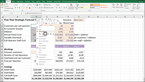
FIGURE 8-4: Using Paste Formulas to retain formatting.

FIGURE 8-5: The completed scenario analysis.
Applying Sensitivity Analysis with Data Tables
Data tables are among the more advanced and complex financial modeling tools available. Data tables can be used for scenarios and sensitivity analysis, but they’re less commonly used because they’re more advanced. Data tables are unlike most other formulas in that you can’t trace dependents, and they’re very difficult to follow unless you’re familiar with them. If anyone you work with doesn’t know data tables, he won’t be able to edit the table or make any changes.
Setting up the calculation
Let’s go back to the profitability model you created in Chapter 6. I recommend that you work through the internal links exercise in Chapter 6, or download the completed version of this model, called File 0603.xlsx, from www.dummies.com/go/financialmodelinginexcelfd first so that you understand how this simple model works before adding sensitivities to it.
Because the model links directly to assumptions, you can use data tables to test the sensitivity of the profit margin to changes in assumptions such as the number of units sold and the cost per unit.
The existing model has a simple Income Statement linking to a number of input variables. You can test the sensitivity of one of the outputs, such as the profit margin, to variations in the input variables. Let’s see how much the profit margin changes when the sales price and cost per unit inputs change. Of course, you could do this manually, but to see the various outputs in a single table, you need to use a data table.
Building a data table with one input
To create a data table in this model, follow these steps:
-
Download File 0802.xlsx from
www.dummies.com/go/financialmodelinginexcelfd, open the file, and select the Assumptions tab.You’re testing how sensitive the profit margin is to changes in the sales price. The inputs for the sales price to be used in the data table have been entered in column A already. The next thing you need to do is to link the output cell to the data table. This needs to go at the top of the data table.
-
Link cell B9 to the profit margin using the formula =‘Summary’!B9.
Don’t type this in — press = and then click the Summary tab, select cell B9, and press Enter.
-
Highlight the entire data table in cells A9:B15, including the output cell, as shown in Figure 8-6.
Note that you must highlight all these cells in order for it to work.
-
Select What-if Analysis from the Data tab and choose Data Table from the options (refer to Figure 8-6).
The Data Table dialog box appears.
Because you’re only doing a one-input data table, you only need to enter data for one variable, but which variable depends on how the data table is arranged and whether the input variable you’re testing is in a row or a column. Because it’s in a column, you should use the Column input cell field.
- Link the column input cell field to the input field for the sales price (cell A4) as shown in Figure 8-7.
-
Click OK.
Your data table populates with the completed sensitivity table, as shown in Figure 8-8.
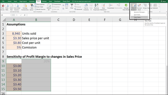
FIGURE 8-6: Selecting the Data Table tool on the Ribbon.

FIGURE 8-7: Linking the one input data table to the input cell.
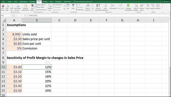
FIGURE 8-8: Completed one-input data table.
Note that the formulas in the data table will have curly brackets around them like this =TABLE{,A4}. This is because it’s an array formula. Array formulas work differently from ordinary formulas because array formulas treat the data like an array instead of a single data value. For this reason, you can’t edit or delete a single cell within a data table in isolation. To make any changes, you need to use the Data Table tool or highlight all the formulas from cell A10 to B15, press Delete, and start again.
Building a data table with two inputs
You can add another input to your data table by listing another input variable across the top. Let’s add the cost per unit as well as the sales price, and this time, we’ll test the total profit (the dollar value) instead of the profit margin (percentage). To complete this sensitivity analysis, follow these steps:
- Scroll down the model to cell A18 and link it to the total profit using the formula =‘Summary’!B8.
-
Highlight the entire data table in cells A18:E24, including the output cell, as shown in Figure 8-9.
Note that again, you must highlight all these cells in order for it to work.
-
Select What-if Analysis from the Data tab and choose Data Table from the options.
The Data Table dialog box appears.
- Link the row input cell field to the input field for the cost per unit (A5) and the column field to the input field for the sales price (A4), as shown in Figure 8-9.
-
Click OK.
Your data table populates with the completed sensitivity table, as shown in Figure 8-10.

FIGURE 8-9: Linking the two-input data table to the input cells.

FIGURE 8-10: Completed two-input data table.
Applying probability weightings to your data table
The great thing about adding a data table to your financial model is that it gives you a large number of variables. However, you know that only one of these can be correct! You can try to reduce the amount of uncertainty by adding probability weightings to a data table because you know that not all outcomes are equally likely.
If you believe certain outcomes to be equally likely, then use the same weighting, while still retaining the probability functionality in the model. For example, if you have four different possible inputs for a data table, simply weight each of them at 25 percent, and the user can change the weighting inputs later.
Build on the data table that you already created in the previous section by following this series of steps:
- Download File 0803.xlsx from
www.dummies.com/go/financialmodelinginexcelfd, open the file, and select the Assumptions tab. -
Enter the probability of each outcome in row 18 and column A, as shown in Figure 8-11.
You may enter any weighting you like as long as the weightings add to 100 percent, but I recommend that you enter the same inputs as those shown in Figure 8-11 so that you can check that the output is accurate.
A check total has been added for you already in cells G18 and A26.
-
Make sure that both column A and row 18 add to 100 percent, and add an error check that will alert the user if it does not because the model will be inaccurate if it does not tally.
You can do this as follows: In cell G19, enter the formula =1-G18, as shown in Figure 8-11, and in cell B26 add the formula =1-A26.
Now add the data table just as you did in the last section.
- Link B19 to the output cell using the formula ='Summary'!B8.
- Highlight the entire range B19:F25.
-
Select the What-if Analysis from the Data tab and choose Data Table from the options.
The Data Table dialog box appears.
-
Link the row field to the input field for the cost per unit (B5) and the column field to the input field for the sales price (B4) and compare your results to those in Figure 8-12.
After you’ve finished the data table, you need to multiply out the probability weightings into the table so that you can work out how likely each outcome is.
-
In cell H20, add the formula =C$18*$A20.
Don’t forget your mixed cell referencing (see Chapter 6).
-
Copy this formula across the block of data to cell K25 and compare your results to those in Figure 8-12.
The total should add to 100 percent.
-
Add an error check in cell L27 with the formula =1-L26.
When the data table and the probability weighting table have been built, you can use the results to calculate the probability weighted outcomes.
-
In cell M20, add the formula =H20*C20.
There is no need to add cell referencing for this calculation.
- Copy this formula across the block of data to cell P25 and compare your results to those in Figure 8-13.
-
In cell Q26, add the entire table together with the formula =SUM(M20:P25), as shown in Figure 8-13.
The calculated result is $5,202, which is the probability weighted predicted outcome of this model. If you’d like to see a completed copy of this model, download File 0804.xlsx from
www.dummies.com/go/financialmodelinginexcelfd.

FIGURE 8-11: Setting up the data table to add probability weightings.
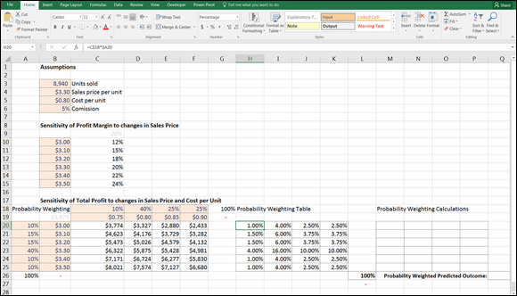
FIGURE 8-12: Building the probability weighting table.

FIGURE 8-13: Completed probability weighted predicted outcome.
Using Scenario Manager to Model Loan Calculations
Scenario Manager is grouped together with Goal Seek and Data Tables in the What-If Analysis section of the Data tab. Being grouped with other tools that are so useful would lead you to believe that Scenario Manager is also a critical tool to know. However, despite its useful-sounding name and the good company it keeps, Scenario Manager is quite limited in its functionality and is as helpful as the name suggests! It’s therefore not frequently used by expert financial modelers; however, for the sake of completeness, I cover it here very briefly.
Setting up the model
To demonstrate how to use Scenario Manager, let’s apply it to a simple loan calculation model. The theory behind loan calculations is quite complex, but fortunately, Excel handles loans quite easily. For more information on modeling loans, interest amounts, and amortization schedules in financial models, see Chapter 6.
In the example shown in Figure 8-14, I’ve created an interest rate calculator upon which you can test the sensitivity of monthly repayments to changes in interest rates and loan terms. Follow these steps:
- Download File 0801.xlsx at
www.dummies.com/go/financialmodelinginexcelfd, open it, and select the tab labeled 8-14, or simply set up the model with hard-coded input assumptions as shown in Figure 8-14. -
In cell B11, type =PMT( and press Ctrl+A.
The Function Arguments dialog box appears.
The PMT function requires the following inputs:
- Rate: The interest rate.
- Nper: The number of periods over the life of the loan.
- Pv: The present value of the loan (the amount borrowed).
- Fv: The amount left at the end of the loan period. (In most cases, you want to pay the entire amount back during the loan period, so you can leave this blank.)
- Type: Whether you want the payments to occur at the beginning or the end of the period. (You can leave this blank for the purposes of this exercise.)
-
Link the fields in the Function Arguments dialog box to the inputs in your model.
The PMT function returns the annual repayment amount. Because you want to calculate the monthly repayment amount, you could simply divide the entire formula by 12, but because the interest is compounding, it’s more accurate to divide each field by 12 within the formula. So, the rate in the first field is converted to a monthly rate, and the number of periods in the second field is also converted to a monthly rate. -
Click OK.
The formula is =PMT(B7/12,B9*12,B5).
This function returns a negative value because this is an expense. For our purposes, change it to a positive by preceding the function with the minus sign.

FIGURE 8-14: Setting up the PMT function to calculate monthly loan repayments.
Applying Scenario Manager
Now you can use Scenario Manager to add some scenarios. You want to know the impact of changes in inputs on your monthly repayments. Follow these steps:
-
On the Data tab, in the Forecast section of the Ribbon, click the What-if Analysis icon, and select Scenario Manager from the drop-down list.
The Scenario Manager dialog box appears.
-
Click the Add button to create a new scenario.
The Add Scenario dialog box, shown in Figure 8-15, appears.
- Enter a name for the first scenario in the Scenario Name box (for example, Scenario One).
-
Enter the cell references for the variable cells in the Changing Cells box, as shown in Figure 8-15.
Separate each reference with a comma (if there is more than one), but don’t use spaces. You can also hold down the Ctrl key and click each cell in the spreadsheet to insert the references into the box.
-
Click OK.
The Scenario Values dialog box appears with the existing values (0.045 for the interest rate and 25 for the years).
- Click OK to accept these values as Scenario One.
-
Click Add to add another scenario.
The Add Scenario dialog box appears again.
- Enter a name for the second scenario in the Scenario Name box (for example, Scenario Two).
-
Click OK.
The Scenario Values dialog box appears again.
- Enter the variables’ values for this scenario (for example, 0.05 for the interest rate and 30 for the years, as shown in Figure 8-16).
-
Click OK.
You’re returned to the Scenario Manager dialog box.
- Follow Steps 7 through 9 again to create additional scenarios.
-
After you’ve created all the scenarios, you can use the Scenario Manager to view each scenario, as shown in Figure 8-17, by clicking the Show button at the bottom.
The inputs are automatically changed to show the scenarios.

FIGURE 8-15: Building the scenario using Scenario Manager.

FIGURE 8-16: Entering scenario values using Scenario Manager.

FIGURE 8-17: The completed Scenario Manager.
Scenarios are sheet-specific, meaning they only exist in the sheet where you created them. So when you’re looking for the scenarios you’ve created, you have to select the correct sheet in the model.