
Chapter 3
Finding and Eliminating Bottlenecks
IN THIS CHAPTER
![]() Identifying the problem
Identifying the problem
![]() Considering possible causes
Considering possible causes
![]() Pondering possible fixes
Pondering possible fixes
![]() Investigating bottlenecks
Investigating bottlenecks
![]() Judging query efficiency
Judging query efficiency
![]() Using resources wisely
Using resources wisely
Databases generally start small and grow with time. Operations that could be performed in a reasonable amount of time with a small database gradually take longer as the database grows. This slowdown probably isn’t due to any general inadequacy of the system, but to a specific link in the chain of operations that leads from a request to a result. That specific link is a bottleneck. Finding and eliminating bottlenecks is one of the main jobs of any person charged with maintaining a database. The ability to determine the cause of a performance shortfall, and to find a remedy, is valuable in any organization and can be highly rewarding, both intellectually and financially.
Pinpointing the Problem
Have you heard the old backwoods story about the frog in hot water? It goes like this:
If you throw a frog into a pot of water that’s practically boiling, it will jump out right away. If, however, you put a frog in a pot that’s at a comfortable temperature and gradually turn up the heat, the frog won’t notice that anything is amiss and will swim around contentedly until it’s too late.
Sometimes, database users are like frogs. When they start using a new database application, they let you know right away if it’s running slowly. If performance is good at first but then gradually degrades, however, they may not notice a difference until that difference is truly dramatic. Some problems manifest themselves right away, whereas others are slow to develop. As you might expect, the causes of the immediate problems tend to be different from the causes of the problems that develop slowly over time. In either case, a database specialist needs to know how to track down the source of the problem and then take appropriate action to fix it.
After the initial loading of data into a database, only two basic activities are performed on it: retrieving a selected portion of the data or updating the data. I count adding new data, deleting existing data, and changing existing data as being forms of updates. Some databases experience many more retrievals, called queries, than they do updates in a given interval. Other databases experience more updates, and some experience about an equal number of queries and updates.
Slow query
Users who are responsible for running queries, like the happily swimming frog, may not notice that their queries are running slower until someone comes by while one is running and remarks on how long it takes for a result to come back. At that point, the users call you. Now you get the chance to do a little detective work. Somewhere — whether it be in the application, the database management system (DBMS), the network link, the database server, or the storage subsystem — something has maxed out. Your job is to figure out what it is and restore performance to acceptable levels as soon as possible without replacing or upgrading the parts of the system that are not part of the problem. Your job is to find the bottleneck.
Slow update
Perhaps the problem is not with queries, but with updates. For a person making additions, changes, or deletions in a database, long waits between entering a change and having the system being ready to accept the next one can be frustrating at best and intolerable at worst. The causes for delays in updating tend to be different from the causes of slow responses to queries. Although the bottleneck may be different, your job is still the same: Find the source of the problem and then fix it. In the next section, I look at some of the likely causes of bottlenecks.
Determining the Possible Causes of Trouble
The main candidates for causing bottlenecks can be categorized in three areas: indexes, communication, and hardware. In this section, I explore these categories further.
Problems with indexes
Probably the number-one cause of less-than-optimal performance is improper indexing. Improper indexing may mean the lack of one or more indexes that should be present, but it could also mean the presence of indexes that should not be there.
B+ tree indexes
Several kinds of indexes exist, but the most common is the B+ tree index, (also called the B-tree index), in which B stands for balanced. A B+ tree has a treelike structure with a root node from which a row of branch nodes fan out. Another row of branch nodes may fan out from the first row, and so on for as many rows as the tree has. The nodes at the end of the chain of branch nodes are called leaf nodes. Leaf nodes have no children; instead, they hold the index values. The root node contains pointers to the first row of branch nodes. The first row of branch nodes contains pointers to the next row of branch nodes. The last row of branch nodes contains pointers to the leaf nodes. The leaf nodes contain pointers to rows in the table being indexed.
Index pluses and minuses
Indexes are valuable because they allow you to find a row in a data table after following a short chain of pointers, as opposed to scanning the table one row at a time until you reach the row you want. The advantage is even greater than it seems on the surface because indexes tend to be small compared with the data tables they’re indexing. This means that the index is often entirely contained in cache memory, which in turn means that the target row in the data table is located at semiconductor RAM speeds rather than mechanical hard disk speeds, as would likely be the case for a full table scan.
The advantages aren’t all on the side of indexing, however. Indexes tend to degrade in tables with frequent inserts and deletes. Deletes create empty leaf nodes, which fill space in cache without contributing and could cause the index to spill out of cache onto the hard disk, with the performance penalty that goes along with that. Eliminating the empty leaf cells requires a time-consuming index rebuild, during which no productive processing can take place.
Updates have an even greater impact on performance than delete operations do. An update that includes at least one indexed column consists of both a delete and an insert. Because an index is a table of pointers, updating an index changes the location of that pointer, requiring its deletion from one place and its insertion at another. Indexes on nonkey columns containing values that change frequently cause the worst performance hits. Updates of indexes on primary keys almost never happen, and updates of indexes on foreign keys are rare. Indexes that aren’t highly selective (such as indexes on columns that contain many duplicates) often degrade overall performance rather than enhance it.
Index-only queries
Indexes have the capability to speed queries because they provide near-direct access to the rows in a data table from which you want to retrieve data. This arrangement is great, but suppose that the data you want to retrieve is entirely contained in the columns that comprise the index. In that case, you don’t need to access the data table at all: Everything you need is contained in the index.
Index-only queries can be very fast indeed, which may make it worthwhile to include in an index a column that you otherwise wouldn’t include, just because it’s retrieved by a frequently run query. In such a case, the added maintenance cost for the index is overshadowed by the increased speed of retrievals for the frequently run query.
Full table scans versus indexed table access
How do you find the rows you want to retrieve from a database table? The simplest way, called a full table scan, is to look at every row in the table, up to the table’s high-water mark, grabbing the rows that satisfy your selection condition as you go. The high-water mark of a table is the largest number of rows it has ever had. Currently, the table may have fewer rows because of deletions, but it still may have rows scattered anywhere up to and including the high-water mark. The main disadvantage of a full table scan is that it must examine every row in the table up to and including the high-water mark. A full table scan may or may not be the most efficient way to retrieve the data you want. The alternative is indexed table access.
As I discuss in the preceding section on the B+ tree index, when your retrieval is on an index, you reach the desired rows in the data table after a short walk through a small number of nodes on the tree. Because the index is likely to be cached, such retrievals are much faster than retrievals that must load sequential blocks from the data table into cache before scanning them.
For very small tables, which are as likely to be cached as an index is, a full table scan is about as fast as an indexed table access. Thus, indexing small tables is probably a bad idea. It won’t gain you significant performance, and it adds complexity and size to your database.
Pitfalls in communication
One area where performance may be lost or gained is in the communication between a database server and the client computers running the database applications. If the communication channel is too narrow for the traffic, or if the channel is just not used efficiently, performance can suffer.
ODBC/JDBC versus native drivers
Most databases support more than one way of connecting to client computers running applications. Because these different ways of connecting employ different mechanisms, they have different performance characteristics. The database application, running on a client computer, must be able to send requests to and receive responses from the database, running on the database server. The conduit for this communication is a software driver that translates application requests into a form that the database can understand and database responses into a form that the application can understand.
You have two main ways of performing this function. One way is to use a native driver, which has been specifically written to interface an application written with a DBMS vendor’s application development tools to that same vendor’s DBMS back end. The advantage of this approach is that because the driver knows exactly what’s required, it performs with minimum overhead. The disadvantage is that an application written with one DBMS back end in mind can’t use a native driver to communicate with a database created with a different DBMS.
In practice, you frequently need to access a database from an application that didn’t originally target that database. In such a case, you can use a generalized driver. The two main types are Open Database Connectivity (ODBC) and Java-Based Database Connectivity (JDBC). ODBC was created by Microsoft but has been widely adopted by application developers writing in the Visual Basic, C, and C++ programming languages. JDBC is similar to ODBC but designed to be used with the Java programming language.
ODBC consists of a driver manager and the specific driver that’s compatible with the target database. The driver performs the ODBC functions and communicates directly with the database server. One feature of the driver manager is its capability to log ODBC calls, which do the actual work of communicating between the application and the database. This feature can be very helpful in debugging a connection, but slows down communication, so it should be disabled in a production environment. ODBC drivers may provide slower performance than a native driver designed to join a specific client with a specific data source. An ODBC driver also may fail to provide all the functions for a specific data source that a native driver would. (I discuss drivers in more detail in Book 5, Chapter 7.)
Locking and client performance
Multiple users can perform read operations without interfering with one another, making use of a shared lock. When an update is involved, however, things are different. As long as an update transaction initiated by one client has a resource in the database locked with an exclusive lock, other clients can’t access that resource. Furthermore, an update transaction can’t place an exclusive lock on a resource that currently is held by a shared lock.
This situation is strong motivation for keeping transactions short. You should consider several factors when you find that a critical resource is being locked too long, slowing performance for everyone. One possibility is that a transaction’s SQL code is written in an inefficient manner, perhaps due to improper use of indexes or poorly written SELECT
Application development tools making suboptimal decisions
Sometimes, an application development tool implements a query differently from what you’d get if you entered the same query directly from the SQL command prompt. If you suspect that lagging performance is due to your development tool, enter the SQL directly, and compare response times. If something that the tool is doing is indeed causing the problem, see whether you can turn off the feature that’s causing extra communication between the client and the server to take place.
Determining whether hardware is robust enough and configured properly
Perhaps your queries are running slowly because your hardware isn’t up to the challenge. It could be a matter of a slow processor, bus clock, or hard disk subsystem, or it could be insufficient memory. Alternatively, your hardware may be good enough but isn’t configured correctly. Your database page buffer may not be big enough, or you may be running in a less-than-optimal mode, such as flushing the page buffer to disk more often than necessary. Perhaps the system is creating checkpoints or database dumps too frequently. All these configuration issues, if recognized and addressed, can improve performance dramatically without touching your equipment budget.
 You may well decide that you need to update some aspect of your hardware environment, but before you do, make sure that the hardware that you already have is configured in such a way that you have a proper balance of performance and reliability.
Implementing General Principles: A First Step Toward Improving Performance
In looking for ways to improve the performance of queries you’re running, some general principles almost always apply. If a query violates any of these principles, you can probably make it run faster by eliminating the violation. Check out the suggestions in this section before expending a lot of effort on other interventions.
Avoid direct user interaction
Among all the components of a database system, the human being sitting at the keyboard is the slowest by far — almost a thousand times slower than a hard disk and more than a billion times slower than semiconductor RAM. Nothing brings a system to its knees as fast as putting a human in the loop. Transactions that lock database resources should never require any action by a human. If your application does require such action, changing your application to eliminate it will do more for overall system performance than anything else you can do.
Examine the application/database interaction
One important performance bottleneck is the communication channel between the server and a client machine. This channel has a design capacity that imposes a speed limit on the packets of information that travel back and forth. In addition to the data that gets transmitted, a significant amount of overhead is associated with each packet. Thus, one large packet is transmitted significantly faster than numerous small packets containing the same amount of information. In practice, this means that it’s better to retrieve the entire set in one shot than to retrieve a set of rows one row at a time. Following that logic, it would be a mistake to put an SQL retrieval statement within a loop in your application program. If you do, you’ll end up sending a request and receiving a response every time through the loop. Instead, grab an entire result set at the same time, and do your processing on the client machine.
Another thing you can do to reduce back-and-forth traffic is to use SQL’s flow of control constructs to execute multiple SQL statements in a single transaction. In this case, the number-crunching takes place on the server rather than on the client. The result is, however, the same as in the preceding paragraph — fewer message packets traveling over the communication channel.
User-defined functions (UDFs) can also reduce client/server traffic. When you include a UDF in a SELECT statement’s WHERE clause, processing is localized in the server, and less data needs to be transmitted to the client. You can create a UDF with a CREATE FUNCTION statement, and then use it as an extension to the SQL language.
Don’t ask for columns that you don’t need
It may seem like a no-brainer to not retrieve columns that you don’t need. After all, doing so shuttles unneeded information across the communications channel, slowing operations. It’s really easy, however, to type the following:
SELECT * FROM CUSTOMER ;
This query retrieves the data you want, along with a lot of unwanted baggage. So work a little harder and list the columns you want — only the columns you want. If it turns out that all the columns you want are indexed, you can save a lot of time, as the DBMS makes an index-only retrieval. Adding just one unindexed column forces the query to access the data table.
Don’t use cursors unless you absolutely have to
Cursors are glacially slow in almost all implementations. If you have a slow-running query that uses cursors, try to find a way to get the same result without cursors. Whatever you come up with is likely to run significantly faster.
Precompiled queries
Compiling a query takes time — often, more than the time it takes to execute the query. Rather than suffer that extra time every time you execute a query, it’s better to suffer it once and then reap the benefit every time you execute the query after the first time. You can do this by putting the query in a stored procedure, which is precompiled by definition.
Precompilation helps most of the time, but it also has pitfalls:
- If an index is added to a column that’s important to a query, you should recompile the query so that it takes advantage of the new index.
- If a table grows from having relatively few rows to having many rows, you should recompile the query. When the query is compiled with few rows, the optimizer probably will choose a full table scan over using an index because for small tables, indexes offer no advantage. When a table grows large, however, an index greatly reduces the execution time of the query.
Tracking Down Bottlenecks
Tracking down bottlenecks is the fun part of database maintenance. You get the same charge that a detective gets from solving a mysterious crime. Breaking the bottleneck and watching productivity go through the roof can be exhilarating.
Your system is crawling when it should be sprinting. It’s a complex construction with many elements, both hardware and software. What should you do first?
Isolating performance problems
As long as a wide variety of system elements could be involved in a problem, it’s hard to make progress. The first step is narrowing down the possibilities. Do this by finding which parts of the system are performing as they should, thus eliminating them as potential sources of the problem. To paraphrase Sherlock Holmes, “When you eliminate all the explanations but one as being not possible, then whatever is left, however unlikely it may seem, must be true.”
Performing a top-down analysis
A query is a multilevel operation, and whatever is slowing it could be at any one of those levels. At the highest level is the query code as implemented in SQL. If the query is written inefficiently, you probably need to look no further for the source of the problem. Rewrite the query more efficiently, and see whether that solves the problem. If it does, great! You don’t have to look any further. If you don’t find an inefficient query, however, or the rewrite doesn’t seem to help, you must dig deeper.
DBMS operations
Below the level of the SQL code is a level where locking, logging, cache management, and query execution take place. All these operations are in the province of the DBMS and are called into action by the top-level SQL. Any inefficiencies here can certainly impact performance, as follows:
- Locking more resources than necessary or locking them for too long can slow operations for everybody.
- Logging is a vital component of the recovery system, and it helps you determine exactly how the system performs, but it also absorbs resources. Excessive logging beyond what’s needed could be a source of slowdowns.
- Cache management is a major factor in overall performance. Are the right pages being cached, and are they remaining in the cache for the proper amount of time?
- Finally, at this level, are queries being executed in the most efficient way? Many queries could be executed a variety of ways and end up with the same result. The execution plans for these different ways can vary widely, however, in how long they take to execute and in what resources they consume while doing it. All these possibilities deserve scrutiny when performance is unacceptable and can’t be attributed to poorly written queries.
Hardware
The lowest level that could contribute to poor performance is the hardware level. Look here after you confirm that everything at the higher levels is working as it should. This level includes the hard disk drives, the disk controller, the processor, and the network. Each of these elements could be a bottleneck if its performance doesn’t match that of the other hardware elements.
HARD DISK DRIVES
The performance of hard disk drives tends to degrade over time, as insertions and deletions are made in databases and as files unrelated to database processing are added, changed, or deleted. The disk becomes increasingly fragmented. If you want to copy a large file to disk, but only small chunks of open space are scattered here and there across the disk’s cylinders, pieces of the file are copied into those small chunks. To read the entire file, the drive’s read/write head must move from track to track, slowing access dramatically. As time goes on, the drive gets increasingly fragmented, imperceptibly at first and then quite noticeably.
The solution to this problem is running a defragmentation utility. This solution can take a long time, and because of heavy disk accessing, it reduces the system’s response time to close to zero. Defragmentation runs should be scheduled at regular intervals when normal traffic is light to maintain reasonable performance. Most modern operating systems include a defragmentation utility that analyzes your hard disk, tells you whether it would benefit from defragmenting, and then (with your consent) performs the defragmentation operation.
DISK CONTROLLER
The disk controller contains a cache of recently accessed pages. When a page that’s already in disk controller cache is requested by the processor, it can be returned much faster than is possible for pages stored only on disk. All the considerations I mention in Book 7, Chapter 2 for optimizing the database page buffer in the processor apply to the disk controller cache as well. The choice of page replacement algorithm can have a major effect on performance, as can cache size.
PROCESSOR
The processor has a tremendous effect on overall system performance because it’s the fastest component in the entire system. Processors just a few years old are significantly slower than those on the market today. Upgrading an older processor, along with all the ancillary circuitry that must be upgraded to support it, can make a significant difference in overall performance.
Many organizations have a regular program of replacing computers at regular intervals, such as every three years. The systems that get replaced are moved down to less-critical applications. This domino effect of hand-me-down computers ends with donation to charitable organizations. If your computer is more than about three years old, consider replacing it as a possible method of improving your performance, assuming that you’ve already investigated all the other sources of slowdown mentioned in this chapter.
NETWORK
The network is the final major subsystem that may be causing performance problems. If the performance of running queries from a client computer on a network is unacceptable, try running the same queries directly on the server. If the queries run significantly faster on the server, the server’s processor may be more powerful, or the network connection between the server and the client may be a bottleneck. Tools for analyzing network traffic can give you some indication whether your network is slowing you.
As is the case with processors, network performance has been increasing steadily. If your network is starting to get a little old, you may be better served by one with state-of-the-art speed. It’s worth looking into.
Partitioning
Suppose that you’ve done the top-down analysis advocated in the preceding section and have isolated your performance problem to one of the primary hardware subsystems: the hard disk drive, disk controller, processor, or network. Suppose further that you’ve done everything you can think of: defragmented your hard drives, optimized paging in your disk controller, optimized paging in your database page buffer, and analyzed the traffic on your network. Despite all these remedies, the problem persists. Partitioning offers another approach that may break the bottleneck.
Partitioning can be helpful if your performance problem is caused by exceeding the capacity of a critical system resource. Partitioning is essentially spreading out the work so that the overstretched resource doesn’t get overloaded.
You can spread the work spatially, temporally, or both. Spatial partitioning means doing more things in parallel, which could entail moving to a multicore processor, adding hard disk drives to your RAID array, installing a bigger database page buffer, and so on. You get the idea. Wherever the bottleneck is, widen the neck to increase the flow rate through it.
The other thing to try is to increase temporal partitioning. In temporal partitioning, you don’t make the neck of the bottle any wider; you just schedule workflow so that it’s more evenly distributed in time. Don’t run large update transactions at the same time that online query activity is high. Give users incentives to use the system across a broader range of times, rather than allow everybody to try to access the same resources at the same time.
Locating hotspots
Spreading the work away from an overloaded resource presupposes that you’re able to determine which of the many components of your system is causing the bottleneck. Such overloaded resources are called hotspots. When a resource is hot, it’s continually in use. If the resource is too hot, operations have to wait in line to use it. If the wait takes too long and results in aborts and rollbacks, performance is greatly affected. Fortunately, several tools are available, both at the operating-system level and at the database level, which you can use to monitor the performance of various aspects of your system and locate the hotspots. These performance monitoring tools, of course, vary from one operating system to another and from one DBMS to another. Check the documentation of your specific systems to determine what is available to you. After you locate a hotspot, you are well on your way to solving your performance problem. When you know what the overloaded system component is, you can apply the remedies discussed in this chapter to restore performance to an acceptable level. In the next section, I discuss several performance monitoring tools available on popular systems.
Analyzing Query Efficiency
Some kinds of problems slow everything that’s running on a system. Other kinds of problems affect the performance of only one query or a few queries. For the class of problems that seem to affect only one or a few queries, the major DBMSs provide tools that you can use to track down the source of the problem. These tools come in three major categories: query analyzers, performance monitors, and event monitors. Each looks at a different aspect of the way a query is running. Based on what these tools tell you, you should be able to zero in on whatever is causing your system to perform less well than it should.
Using query analyzers
All the major DBMSs offer tools that give the database administrator (or other person responsible for the efficient operation of the database) a way of analyzing how well queries on the database are performing. In versions of Microsoft SQL Server before SQL Server 2005, the tool for this job was even named Query Analyzer. SQL Server 2005 represented a major break from the past in a number of ways. The functions that had been the province of Query Analyzer were incorporated into the new Microsoft SQL Server Management Studio, along with additional functionality useful for tuning query performance. This functionality is retained, along with a lot of other functionality in the version of SQL Server Management Studio included with SQL Server 2017.
Here’s a brief introduction to SQL Server 2017’s tuning tools (the Database Engine Tuning Advisor and the SQL Server Profiler) to give you an idea of what such tools look like and what they do. The operation of the tuning tools in SQL Server Management Studio differs in detail from the operation of similar tools for other DBMSs, but the overall functions are the same.
Figure 3-1 shows the main screen of Microsoft SQL Server Management Studio.
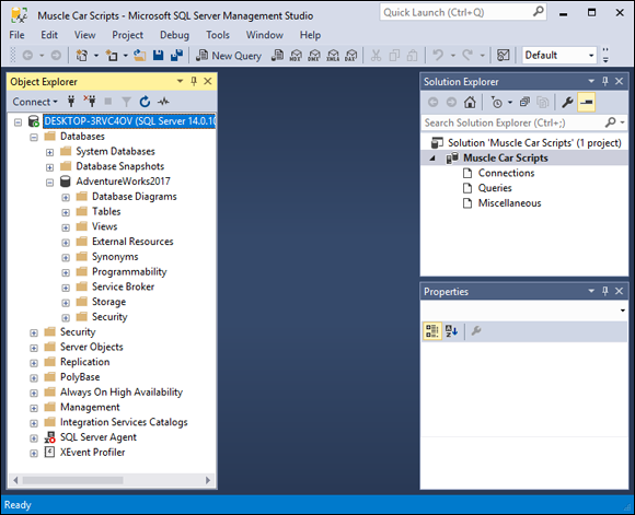
FIGURE 3-1: Microsoft SQL Server Management Studio.
If you take a peek at the Object Explorer in the left pane of the Management Studio window (refer to Figure 3-1), you can see that I’ve connected to a database named AdventureWorks2017. This database is a sample SQL Server database provided by Microsoft. If you don’t have it already, you can download it from www.msdn.microsoft.com. It contains sample data for a fictitious company.
Suppose that you’re a manager at AdventureWorks, and you want to know what customers you have in the United States. You can find out with a simple SQL query. To draft a query in Management Studio, follow these steps:
Click the New Query button at the left end of the Standard toolbar.
An SQL editor pane opens in the middle of the Management Studio window, as shown in Figure 3-2.
 To remind yourself of the names of the tables in the AdventureWorks2017 database, you can expand the Databases node and then, from the items that appear below it, expand the Tables node in the tree in the Object Explorer in the left pane of the Management Studio window.
Type your query in the editor pane, as shown in Figure 3-3.
The query
SELECT FirstName, LastName, Phone FROM Person.ContactWHERE LastName = 'Taylor' ;retrieves the names and phone numbers of everybody in the Contact table of the Person schema whose last name is Taylor.
Execute the query by clicking the Execute button in the toolbar.
The result of the query shows up in the Results tab, as shown in Figure 3-4. The first several of the 83 people in the table whose last name is Taylor appear on the tab. You can see the rest by scrolling down.
The tree at the left shows that the Phone column is a nullable
VARCHARfield and that the primary key of the Contact table is ContactID. The Phone column isn’t indexed. There are indexes on rowguid, EmailAddress, the primary key PK_Customers, and AddContact. None of these indexes is of any use for this query — an early clue that performance of this query could be improved by tuning.Name and save your query by choosing File ⇒ Save As.
My example query is named
SQLQuery2.sql. You can name yours whatever you want.
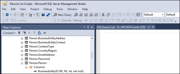
FIGURE 3-2: The Microsoft SQL Server Management Studio SQL editor pane.
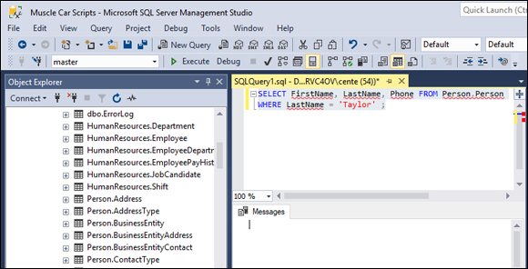
FIGURE 3-3: A sample query.

FIGURE 3-4: The query result.
Now you have a sample query that’s ready to be taken through its paces. The next sections spell out how SQL Server Management Studio lets you do that.
The Database Engine Tuning Advisor
The tool that SQL Server Management Studio provides for tuning queries is the Database Engine Tuning Advisor. To use this tool with the sample query created in the preceding section, follow these steps:
In SQL Server Management Studio, choose Tools ⇒ Database Engine Tuning Advisor.
The Tuning Advisor window opens to the General tab, as shown in Figure 3-5.
- When you’re asked to connect to the server you’re using, do so.
- (Optional) The system has assigned a default session name, based on your login and the date and time; change this session name if you want to.
- In the Workload section, choose the File radio button and then click the Browse for a Workload File button to the right of the long text box.
Find and select the query file that you just created.
For this example, I select
SQLQuery2.sql.Choose your database from the Database for workload analysis drop-down menu.
For this example, I choose AdventureWorks2017.
- In the list of databases at the bottom of the Tuning Advisor window, select the check box next to the name of your database.
Make sure that the Save Tuning Log check box (at the bottom of the list of databases) is selected.
This option creates a permanent record of the tuning operation that’s about to take place. Figure 3-6 shows what the Tuning Advisor window should look like at this point.
Click the Tuning Options tab to see what the default tuning options are — and to change them, if so desired.
Figure 3-7 shows the contents of the Tuning Advisor’s Tuning Options tab.
The Limit Tuning Time check box in the top left corner is selected by default: Tuning can be so time-consuming that it severely affects normal production operation. To prevent this effect, you can set the maximum amount of time that a tuning session can take. When that maximum is reached, whatever tuning recommendations have been arrived at so far are shown as the result. If the tuning run had been allowed to run to completion, different recommendations might have been made. If your server is idle or lightly loaded, you may want to clear this check box to make sure that you get the best recommendation.The three tuning options you can change are
- Physical Design Structures (PDS) to use in database: The Indexes radio button is selected, and other options are either not selected or not available. For the simple query you’re considering, indexes are the only PDS that it makes sense to use.
- Partitioning Strategy to employ: No partitioning is selected. Partitioning means breaking up tables physically across multiple disk drives, which enables multiple read/write heads to be brought into play in a query, thereby speeding access. Depending on the query and the clustering of data in tables, partitioning may enhance performance. Partitioning isn’t applicable if the entire database is contained on a single disk drive, of course.
- Physical Design Structures (PDS) to keep in database: Here, you can specify which PDSs to keep. The Tuning Advisor may recommend dropping other structures (such as indexes or partitioning) that aren’t contributing to performance.
Click the Advanced Options button to open the Advanced Tuning Options dialog box.
The Advanced Tuning Options dialog box (see Figure 3-8) enables you to specify a maximum amount of memory use for the recommendations. In the process of coming up with a recommendation, the Tuning Advisor can consume considerable memory. If you want to set a limit on the amount it can commandeer, this dialog box is the place to do it. (The Online Index Recommendations check boxes allow you to specify where you want to see any recommendations for indexes that are generated.)
Click OK to return to the General tab (refer to Figure 3-6), confirm that your query file is specified in the Workload area, and then click the Start Analysis button to commence tuning.
The Start Analysis button is in the icon bar, just below the Actions option on the main menu.
Depending on the sizes of the tables involved in the query, this process could take a significant amount of time. The Tuning Advisor keeps you apprised on progress as the session runs.

FIGURE 3-5: The Database Engine Tuning Advisor window.
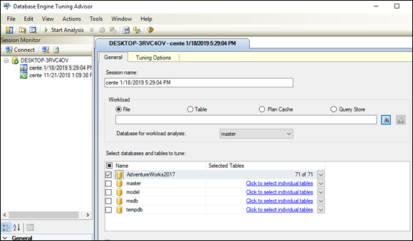
FIGURE 3-6: The Tuning Advisor window, ready to tune a query.
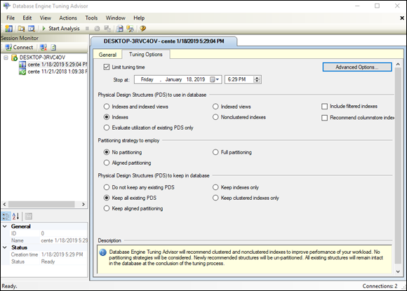
FIGURE 3-7: The Tuning Options pane.
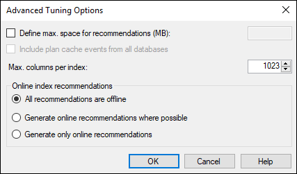
FIGURE 3-8: Advanced tuning options.
Figure 3-9 shows the Progress tab at the end of a successful run. It shows up after a tuning run starts.

FIGURE 3-9: The Progress tab after a successful run.
Figure 3-10 shows the Recommendations tab, which appears when a tuning run is complete.
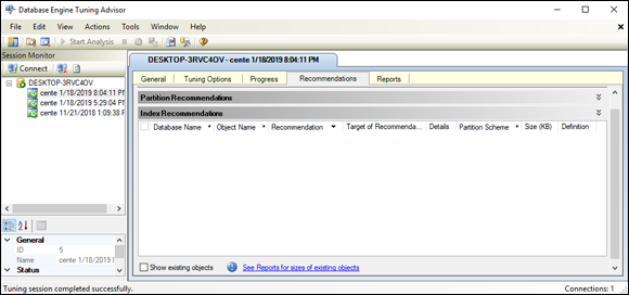
FIGURE 3-10: The Recommendations tab after a successful run.
In Figure 3-10, the Tuning Advisor has concluded that tuning would not improve performance at all. The query is already as efficient as it can be.
When you complete the tuning run, you’ll probably want to look at the Reports tab, which is shown in Figure 3-11.

FIGURE 3-11: The Reports tab after a successful run.
In this report, you see the details of the tuning run. The report in Figure 3-11, for example, shows that 1 minute of tuning time was used and that the Tuning Advisor expects 0.00 percent improvement if you perform any tuning. The Tuning Advisor’s recommendation allocates a maximum 279MB of space. Currently, the table uses 180MB of space. If the memory allocated originally was too small, it’s a simple matter to raise the limit. Finally, note that 100 percent of the SELECT statements were in the tuned set — a confirmation that the tuning session ran to completion.
SQL Server Profiler
The Database Engine Tuning Advisor is just one tool that SQL Server Management Studio provides to help you optimize your queries. The SQL Server Profiler is another tool available under the Tools tab. Instead of operating on SQL scripts, it traces the internal operation of the database engine on a query, showing exactly what SQL statements are submitted to the server — which may differ from the statements written by the SQL programmer — and how the server accesses the database.
After you start a trace in the Profiler by choosing File ⇒ New Trace, it traces all DBMS activity until you tell it to stop. Somewhere among all the things that are going on, actions relevant to your query are recorded. Figure 3-12 shows the General tab of the Trace Properties dialog box, which appears when you select New Trace.

FIGURE 3-12: The Trace Properties dialog box.
Figure 3-13 shows the Events Selection tab of the Trace Properties dialog box. In this example, the default selections are shown, selecting almost everything to be recorded. In many cases, this selection is overkill, so you should deselect the things that don’t interest you. Click the Run button to start the trace, and then click the Execute button in Management Studio to give the trace a query to operate upon.
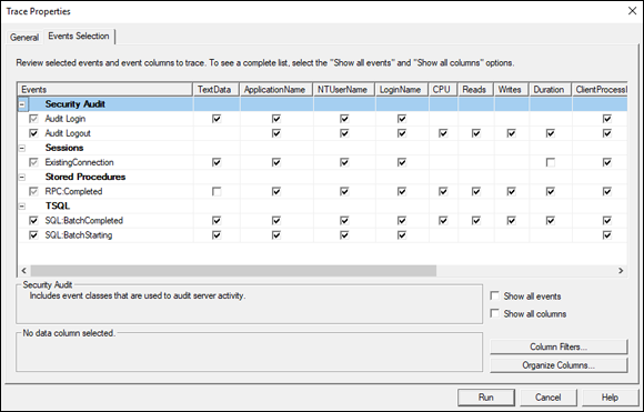
FIGURE 3-13: The Events Selection tab of the Trace Properties dialog box.
A trace of SQLQuery2.sql dumps information about the EventClasses that you’ve specified for monitoring. Figure 3-14 is a view of the trace, showing the events that I selected. Data listed on the right side of the trace window include CPU usage, number of reads, number of writes, and time consumed by every event represented by a row in the trace file.
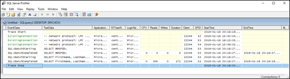
FIGURE 3-14: Trace for a simple query.
You can include many more event classes in a trace beyond the few that I display in this section. Check the Show All Events box in the Events Selection pane of the Trace Properties dialog box to display a host of them. You can break down a query to its constituent parts and see which parts are consuming the most time and resources. For the trace shown in Figure 3-14, I chose to monitor the acquisition and release of locks (and there were a lot of them). In cases in which you have little or no chance of deadlocks or lock contention, the trace will run faster if you choose not to monitor lock behavior.
Queries aren’t the only things that consume system resources. If you’re experiencing performance problems, the source of the problem may be somewhere other than in a poorly performing query. Performance monitors are tools that give you a broader view of how a system is performing. Just remember that performance monitors aren’t specifically related to database systems but are maintained by the operating system.
The Oracle Tuning Advisor
The Oracle Tuning Advisor analyzes a query presented to it and issues recommendations for rewriting it to improve performance. The learning curve for this tool is somewhat steeper than that for the SQL Server Database Engine Tuning Advisor, but after you master the syntax, it provides very helpful recommendations.
Finding problem queries
In a poorly performing multiuser, multitasking environment in which multiple queries are being run at any given moment, tracking the source of the problem may be difficult. Is the problem systemic? Are weaknesses in the server’s processor, the server’s memory, or the network slowing everything? Is one problem query gumming up the works for everyone? This last question is particularly important. If you can restore performance to a satisfactory level by tuning a query, doing so is a lot cheaper than making a major hardware upgrade that may not solve the problem.
A useful approach is the divide-and-conquer strategy. Find all the jobs that typically run together when performance is slow, and run them individually. Use your system’s performance-monitoring tools to check for jobs that saturate one or more system resources. Then use your event-monitoring tool to find a query that seems to be consuming more time and resources than it should.
When you find a suspicious query, use your query-analyzer tool to look inside the query to see exactly where time and resources are being consumed. When you find a bad actor, you can try several things to make matters better. In the next sections, I discuss a few of those techniques.
Analyzing a query’s access plan
A DBMS generates an access plan that describes how to execute a query. The details of the access plan depend on what the DBMS knows or can assume about what system resources are available and what the query needs. This knowledge is largely based on statistics that show how the system has been running lately on queries similar to the one for which the access plan is being developed.
CHECKING THE ACCESS PATH
After the query optimizer generates an access plan, check the plan to see how the query accesses table rows. Is it doing a full table scan? If a full table scan of a large table uploads a big chunk of the table into the database buffer, it could push data out of the buffer that other queries running concurrently will need soon. This situation won’t show up as a performance bottleneck for the query you’re looking at, but it affects the performance of the other queries running at the same time.
Interactions of this type are devilishly difficult to unravel and fix. Some DBMSs are smart enough to recognize this situation, and instead of following the normal practice of flushing the least recently used (LRU) pages from the buffer, they page out the big chunk because it’s unlikely to be needed again soon after the scan.
In most situations, unless you’re dealing with a very small table, indexed access is better than a full table scan. If your query’s access plan specifies a full table scan, examine the plan carefully to see whether indexed access would be better. It may make sense to create a new index if the appropriate index doesn’t exist.
Here are several reasons why indexed access tends to be better:
- The target of an indexed access is almost always cached.
- Table blocks reached by an index tend to be hotter than other blocks and consequently are more likely to be cached. These rows, after all, are the ones that you (and possibly other users) are hitting.
- Full table scans cache a multiblock group, whereas an indexed access retrieves a single block. The single blocks retrieved by indexed access are likelier to contain the rows that you and other users need than are blocks in a multiblock group that came along for the ride in a full table scan.
- Indexed accesses look only at the rows that you want in a retrieved block rather than every row in the block, thus saving time.
- Indexed accesses scale better than full table scans, which become worse as table size increases.
Full table scans make sense if you’re retrieving 20 percent or more of the rows in a table. Indexed retrievals are clearly better if you’re retrieving 0.5 percent or fewer of the rows in the table. Between those two extremes, the best choice depends on the specific situation.
FILTERING SELECTIVELY
Conditions such as those in an SQL WHERE clause act as filters. They exclude the table rows that you don’t want and pass on for further processing the rows that you may want. If a condition specifies a range of index values for further processing, values outside that range need not be considered, and the data table itself need not be accessed as part of the filtering process. This filter is the most efficient kind because you need to look only at the index values that correspond to the rows in the data table that you want.
If the desired index range isn’t determined by the condition, but rows to be retrieved are determinable from the index, performance can still be high because, although index values that are ultimately discarded must be accessed, the underlying data table needn’t be touched.
Finally, if rows to be retrieved can’t be determined from the index but require table access, no time is saved in the filtering process, but network bandwidth is saved because only the filtered rows need to be sent to the requesting client.
CHOOSING THE BEST JOIN TYPE
In Book 3, Chapter 4, I discuss several join types. Although the SQL code may specify one of the join types discussed there, the join operation that’s actually executed is probably one of three basic types: nested-loops, hash, or sort-merge. The Query optimizer chooses one of these join types for you. In most cases, it chooses the type that turns out to be the best. Still, you should understand the three types and what distinguishes them from one another, as follows:
- Nested-loops join: A nested-loops join is a robust method of joining tables that almost always produces results in close to the shortest possible time. It works by filtering unwanted rows from one table (the driving table) and then joining the result to a second table, filtering out unwanted rows of the result in the process, joining the result to the next table, and so on until all tables have been joined and the fully filtered result is produced.
- Hash join: In some situations, a hash join may perform better than a nested-loops join. This situation occurs when the smaller of the two tables being joined is small enough to fit entirely into semiconductor memory. Unwanted rows are discarded from the smaller table, and the remaining rows are placed in buckets according to a hashing algorithm. At the same time, the larger driving table is filtered; the remaining rows are matched to the rows from the smaller table in the hash buckets; and unmatched rows are discarded. The matched rows form the result set.
- Sort-merge join: A sort-merge join reads two tables independently, discarding unwanted rows. First, it presorts both tables on the join key and merges the sorted lists. The presort operation is expensive in terms of time, so unless you can guarantee that both tables will fit into semiconductor memory, this technique performs worse than a hash join of the same tables.
Examining a query’s execution profile
Perhaps you’ve examined an expensive query’s access plan and found it to be about as efficient as can be expected. The next step is looking at the query’s execution profile — the accounting information generated by the profiler. Among the pieces of information available are the number of physical and logical reads and the number of physical and logical writes. Logical operations are those that read or write memory. Physical operations are logical operations that go out to disk.
Other information available in the profile includes facts about locking. Of interest are the number of locks held and the length of time they’re held. Time spent waiting for locks, as well as deadlocks and timeouts, can tell you a lot about why execution is slow.
Sorts are also performance killers. If the profile shows a high number of sorts or large areas of memory used for sorting, this report is a clue that you should pursue.
Resource contention between concurrently running transactions can drag down the performance of all transactions, which provides excellent motivation to use resources wisely, as I discuss in the following section.
Managing Resources Wisely
The physical elements of a database system can play a major role in how efficiently the database functions. A poorly configured system performs well below the performance that’s possible if it’s configured correctly. In this section, I review the roles played by the various key subsystems.
The disk subsystem
The way that data is distributed across the disks in a disk subsystem affects performance. The ideal case is to store contiguous pages on a single cylinder of a disk to support sequential prefetching — grabbing pages from disk before you need them. Spreading subsequent pages to similarly configured disks enables related reads and writes to be made in parallel. A major cause of performance degradation is disk fragmentation caused by deletions opening free space in the middle of data files that are then filled with unrelated file segments. This situation causes excessive head seeks, which slow performance dramatically. Disk fragmentation can accumulate rapidly in transaction-oriented environments and can become an issue over time even in relatively static systems.
Tools for measuring fragmentation are available at both the operating-system and database levels. Operating-system defragmentation tools work on the entire disk, whereas database tools measure the fragmentation of individual tables. An example of an operating-system defragmentation tool is the tool for Microsoft Windows, Optimize Drives utility, which you can access from the Search field. Figure 3-15 shows the result of an analysis of a slightly fragmented C: drive, an unfragmented backup drive, and a 28% fragmented System drive. Optimizing the System drive will improve performance.

FIGURE 3-15: An Optimize Drives display of a computer’s disk drives.
In addition to being badly fragmented, this drive has very little free space, and none of that space is in large blocks, which makes it almost impossible to store a new database in a fragment-free manner.
With Optimize Drives, you can not only analyze the fragmentation of a disk drive, but also defragment it. Alas, this defragmentation usually is incomplete. Files that Optimize Drives can’t relocate continue to impair performance.
DBMSs also have fragmentation analysis tools, but they concentrate on the tables in a database rather than look at the entire hard disk. SQL Server, for example, offers the sys.dm_db_index_physical_stats command, which returns size and fragmentation data for the data and indexes of a specified table or view. It doesn’t fix the fragmentation; it only tells you about it. If you decide that fragmentation is excessive and is impairing performance, you must use other tools — such as the operating-system defragmentation utility — to remedy the situation.
The database buffer manager
The job of the buffer manager is to minimize the number of disk accesses made by a query. It does this by keeping hot pages — pages which have been used recently and are likely to be used again soon — in the database buffer while maintaining a good supply of free pages in the buffer. The free pages provide a place for pages that come up from disk without the need to write a dirty page back to disk before the new page can be brought in.
You can see how good a job the buffer manager is doing by looking at the cache–hit ratio — the number of times a requested page is found in the buffer divided by the total number of page requests. A well-tuned system should have a cache–hit ratio of more than 90 percent.
In the specific case of Microsoft SQL Server running under Microsoft Windows, you can monitor the cache–hit ratio along with many other performance parameters from the Windows System Monitor. You can access the System Monitor from the Windows command prompt by typing perfmon. This launches the System Monitor in a window titled Reliability and Performance Monitor. From the menu tree on the left edge of the window, under Monitoring Tools, select Performance Monitor. This displays the Performance Monitor Properties dialog box. Open the Data tab and then click the Add button. This enables you to add counters that monitor many performance-related quantities, including cache–hit ratio.
Activating the System Monitor consumes resources, which affects performance. Use it when you are tracking down a bottleneck, but turn it off when you are finished before returning to normal operation.
Another useful metric is the number of free pages. If you check the cache–hit ratio and the number of free pages frequently under a variety of load conditions, you can keep an eye out for a trend that could lead to poor performance. Addressing such problems sooner rather than later is wise. With the knowledge you gain from regular monitoring of system health, you can act in a timely manner and maintain a satisfactory level of service.
The logging subsystem
Every transaction that makes an insertion, alteration, or deletion in the database is recorded in the log before the change is actually made in the database. This recovery feature permits reconstruction of what occurred before a transaction abort or system failure. Because the log must be written to before every action that’s taken on the database, it’s a potential source of slowdown if log writes can’t keep up with the transaction traffic. Use the performance-monitoring tools available to you to confirm that there are no holdups due to delays in making log entries.
The locking subsystem
The locking subsystem can affect performance if multiple transactions are competing to acquire locks on the same object. If a transaction holds a lock too long, other transactions may time out, necessitating an expensive rollback.
You can track down the source of locking problems by checking statistics that are normally kept by the DBMS. Some helpful statistics are
- Average lock wait time (the average amount of time a transaction must wait to obtain a lock)
- Number of transactions waiting for locks
- Number of timeouts
- Number of deadlocks
Time spent waiting for locks should be low compared with total transaction time. The number of transactions waiting for locks should be low compared with the number of active transactions.
If the metrics cited here point to a problem with locks, you may be able to trace the source of the problem with a Microsoft Windows System Monitor or the equivalent event monitor in a different operating environment. Things such as timeouts and deadlocks appear in the event log and indicate what was happening when the event occurred.