Chapter 2
SELECT Statements and Modifying Clauses
IN THIS CHAPTER
![]() Retrieving data from a database
Retrieving data from a database
![]() Zeroing in on what you want
Zeroing in on what you want
![]() Optimizing retrieval performance
Optimizing retrieval performance
The main purpose of storing data on a computer is to be able to retrieve specific elements of the data when you need them. As databases grow in size, the proportion that you are likely to want on any given occasion becomes smaller. As a result, SQL provides tools that enable you to make retrievals in a variety of ways. With these tools — SELECT statements and modifying clauses — you can zero in on the precise pieces of information that you want, even though they may be buried among megabytes of data that you’re not interested in at the moment.
Finding Needles in Haystacks with the SELECT Statement
SQL’s primary tool for retrieving information from a database is the SELECT statement. In its simplest form, with one modifying clause (a FROM clause), it retrieves everything from a table. By adding more modifying clauses, you can whittle down what it retrieves until you are getting exactly what you want, no more and no less.
Suppose you want to display a complete list of all the customers in your CUSTOMER table, including every piece of data that the table stores about each one. That is the simplest retrieval you can do. Here’s the syntax:
SELECT * FROM CUSTOMER ;
The asterisk (*) is a wildcard character that means all columns. This statement returns all the data held in all the rows of the CUSTOMER table. Sometimes that is exactly what you want. At other times, you may only want some of the data on some of the customers: those that satisfy one or more conditions. For such refined retrievals, you must use one or more modifying clauses.
Modifying Clauses
In any SELECT statement, the FROM clause is mandatory. You must specify the source of the data you want to retrieve. Other modifying clauses are optional. They serve several different functions:
- The
WHEREclause specifies a condition. Only those table rows that satisfy the condition are returned. - The
GROUPBYclause rearranges the order of the rows returned by placing rows together that have the same value in a grouping column. - The
HAVINGclause filters out groups that do not meet a specified condition. - The
ORDERBYclause sorts whatever is left after all the other modifying clauses have had a chance to operate.
The next few sections look at these clauses in greater detail.
FROM clauses
The FROM clause is easy to understand if you specify only one table, as in the previous example.
SELECT * FROM CUSTOMER ;
This statement returns all the data in all the rows of every column in the CUSTOMER table. You can, however, specify more than one table in a FROM clause. Consider the following example:
SELECT *
FROM CUSTOMER, INVOICE ;
This statement forms a virtual table that combines the data from the CUSTOMER table with the data from the INVOICE table. Each row in the CUSTOMER table combines with every row in the INVOICE table to form the new table. The new virtual table that this combination forms contains the number of rows in the CUSTOMER table multiplied by the number of rows in the INVOICE table. If the CUSTOMER table has 10 rows and the INVOICE table has 100, the new virtual table has 1,000 rows.
This operation is called the Cartesian product of the two source tables. The Cartesian product is a type of JOIN. I cover JOIN operations in detail in Chapter 4 of this minibook.
In most applications, the majority of the rows that form as a result of taking the Cartesian product of two tables are meaningless. In the case of the virtual table that forms from the CUSTOMER and INVOICE tables, only the rows where the CustomerID from the CUSTOMER table matches the CustomerID from the INVOICE table would be of any real interest. You can filter out the rest of the rows by using a WHERE clause.
Row pattern recognition is a new capability that was added to the FROM clause in SQL:2016. It enables you to find patterns in a data set. The capability is particularly useful in finding patterns in time series data, such as stock market quotes or any other data set where it would be helpful to know when a trend reverses direction. The row pattern recognition operation is accomplished with a MATCH_RECOGNIZE clause within an SQL statement’s FROM clause. The syntax of the row pattern recognition operation is more complex than I want to get into in this overview of modifying clauses. It is described in detail in ISO/IEC TR 19075-5:2016(E), Section 3, which is available for free from ISO. As of this writing, of the major RDBMS products, only Oracle implements row pattern recognition.
WHERE clauses
I use the WHERE clause many times throughout this book without really explaining it because its meaning and use are obvious: A statement performs an operation (such as a SELECT, DELETE, or UPDATE) only on table rows where a stated condition is TRUE. The syntax of the WHERE clause is as follows:
SELECT <i>column_list</i>
FROM <i>table_name</i>
WHERE <i>condition</i> ;
DELETE FROM <i>table_name</i>
WHERE <i>condition</i> ;
UPDATE <i>table_name</i>
SET column<sub>1</sub>=value<sub>1</sub>, column<sub>2</sub>=value<sub>2</sub>, …, column<sub>n</sub>=value<sub>n</sub>
WHERE <i>condition</i> ;
The condition in the WHERE clause may be simple or arbitrarily complex. You may join multiple conditions together by using the logical connectives AND, OR, and NOT (which I discuss later in this chapter) to create a single condition.
The following statements show you some typical examples of WHERE clauses:
WHERE CUSTOMER.CustomerID = INVOICE.CustomerID
WHERE MECHANIC.EmployeeID = CERTIFICATION.MechanicID
WHERE PART.QuantityInStock < 10
WHERE PART.QuantityInStock > 100 AND PART.CostBasis > 100.00
The conditions that these WHERE clauses express are known as predicates. A predicate is an expression that asserts a fact about values.
The predicate PART.QuantityInStock < 10, for example, is True if the value for the current row of the column PART.QuantityInStock is less than 10. If the assertion is True, it satisfies the condition. An assertion may be True, False, or UNKNOWN. The UNKNOWN case arises if one or more elements in the assertion are null. The comparison predicates (=, <, >, <>, <=, and >=) are the most common, but SQL offers several others that greatly increase your capability to distinguish, or filter out, a desired data item from others in the same column. The following list notes the predicates that give you that filtering capability:
- Comparison predicates
BETWEENIN [NOT IN]LIKE [NOT LIKE]NULLALL,SOME, andANYEXISTSUNIQUEDISTINCTOVERLAPSMATCH
The mechanics of filtering can get a bit complicated, so let me take the time to go down this list and explain the mechanics of each predicate.
Comparison predicates
The examples in the preceding section show typical uses of comparison predicates in which you compare one value to another. For every row in which the comparison evaluates to a True value, that value satisfies the WHERE clause, and the operation (SELECT, UPDATE, DELETE, or whatever) executes upon that row. Rows that the comparison evaluates to FALSE are skipped. Consider the following SQL statement:
SELECT * FROM PART
WHERE QuantityInStock < 10 ;
This statement displays all rows from the PART table that have a value of less than 10 in the QuantityInStock column.
Six comparison predicates are listed in Table 2-1.
TABLE 2-1 SQL’s Comparison Predicates
Comparison |
Symbol |
Equal |
= |
Not equal |
<> |
Less than |
< |
Less than or equal |
<= |
Greater than |
> |
Greater than or equal |
>= |
BETWEEN
Sometimes, you want to select a row if the value in a column falls within a specified range. One way to make this selection is by using comparison predicates. For example, you can formulate a WHERE clause to select all the rows in the PART table that have a value in the QuantityInStock column greater than 10 and less than 100, as follows:
WHERE PART.QuantityInStock > 10 AND PART.QuantityInStock < 100
This comparison doesn’t include parts with a quantity in stock of exactly 10 or 100 — only those values that fall in between these two numbers. To include the end points, you can write the statement as follows:
WHERE PART.QuantityInStock >= 10 AND PART.QuantityInStock <= 100
Another (potentially simpler) way of specifying a range that includes the end points is to use a BETWEEN predicate, like this:
WHERE PART.QuantityInStock BETWEEN 10 AND 100
This clause is functionally identical to the preceding example, which uses comparison predicates. This formulation saves some typing and is a little more intuitive than the one that uses two comparison predicates joined by the logical connective AND.
 The
The BETWEEN keyword may be confusing because it doesn’t tell you explicitly whether the clause includes the end points. In fact, the clause does include these end points. BETWEEN also fails to tell you explicitly that the first term in the comparison must be equal to or less than the second. If, for example, PART.QuantityInStock contains a value of 50, the following clause returns a TRUE value:
WHERE PART.QuantityInStock BETWEEN 10 AND 100
However, a clause that you may think is equivalent to the preceding example returns the opposite result, False:
WHERE PART.QuantityInStock BETWEEN 100 AND 10
 If you use
 BETWEEN, you must be able to guarantee that the first term in your comparison is always equal to or less than the second term.
You can use the BETWEEN predicate with character, bit, and datetime data types as well as with the numeric types. You may see something like the following example:
SELECT FirstName, LastName
FROM CUSTOMER
WHERE CUSTOMER.LastName BETWEEN 'A' AND 'Mzzz' ;
This example returns all customers whose last names are in the first half of the alphabet.
IN and NOT IN
The IN and NOT IN predicates deal with whether specified values (such as GA, AL, and MS) are contained within a particular set of values (such as the states of the United States). You may, for example, have a table that lists suppliers of a commodity that your company purchases on a regular basis. You want to know the phone numbers of those suppliers located in the southern United States. You can find these numbers by using comparison predicates, such as those shown in the following example:
SELECT Company, Phone
FROM SUPPLIER
WHERE State = 'GA' OR State = 'AL' OR State = 'MS' ;
You can also use the IN predicate to perform the same task, as follows:
SELECT Company, Phone
FROM SUPPLIER
WHERE State IN ('GA', 'AL', 'MS') ;
This formulation is more compact than the one using comparison predicates and logical OR.
The NOT IN version of this predicate works the same way. Say that you have locations in New York, New Jersey, and Connecticut, and to avoid paying sales tax, you want to consider using suppliers located anywhere except in those states. Use the following construction:
SELECT Company, Phone
FROM SUPPLIER
WHERE State NOT IN ('NY', 'NJ', 'CT') ;
Using the IN keyword this way saves you a little typing. Saving a little typing, however, isn’t that great an advantage. You can do the same job by using comparison predicates, as shown in this section’s first example.
 You may have another good reason to use the
 IN predicate rather than comparison predicates, even if using IN doesn’t save much typing. Your DBMS probably implements the two methods differently, and one of the methods may be significantly faster than the other on your system. You may want to run a performance comparison on the two ways of expressing inclusion in (or exclusion from) a group and then use the technique that produces the quicker result. A DBMS with a good optimizer will probably choose the more efficient method, regardless of which kind of predicate you use. A performance comparison gives you some idea of how good your DBMS’s optimizer is. If a significant difference between the run times of the two statements exists, the quality of your DBMS’s optimizer is called into question.
The IN keyword is valuable in another area, too. If IN is part of a subquery, the keyword enables you to pull information from two tables to obtain results that you can’t derive from a single table. I cover subqueries in detail in Chapter 3 of this minibook, but following is an example that shows how a subquery uses the IN keyword.
Suppose that you want to display the names of all customers who’ve bought the flux capacitor product in the last 30 days. Customer names are in the CUSTOMER table, and sales transaction data is in the PART table. You can use the following query:
SELECT FirstName, LastName
FROM CUSTOMER
WHERE CustomerID IN
(SELECT CustomerID
FROM INVOICE
WHERE SalesDate >= (CurrentDate – 30) AND InvoiceNo IN
(SELECT InvoiceNo
FROM INVOICE_LINE
WHERE PartNo IN
(SELECT PartNo
FROM PART
WHERE NAME = 'flux capacitor' ) ;
The inner SELECT of the INVOICE table nests within the outer SELECT of the CUSTOMER table. The inner SELECT of the INVOICE_LINE table nests within the outer SELECT of the INVOICE table. The inner select of the PART table nests within the outer SELECT of the INVOICE_LINE table. The SELECT on the INVOICE table finds the CustomerID numbers of all customers who bought the flux capacitor product in the last 30 days. The outermost SELECT (on the CUSTOMER table) displays the first and last names of all customers whose CustomerID is retrieved by the inner SELECT statements.
LIKE and NOT LIKE
You can use the LIKE predicate to compare two character strings for a partial match. Partial matches are valuable if you don’t know the exact form of the string for which you’re searching. You can also use partial matches to retrieve multiple rows that contain similar strings in one of the table’s columns.
To identify partial matches, SQL uses two wildcard characters. The percent sign (%) can stand for any string of characters that have zero or more characters. The underscore (_) stands for any single character. Table 2-2 provides some examples that show how to use LIKE.
TABLE 2-2 SQL’s LIKE Predicate
Statement |
Values Returned |
|
auto |
automotive |
|
automobile |
|
automatic |
|
autocracy |
|
|
code of conduct |
model citizen |
|
|
mope |
tote |
|
rope |
|
love |
|
cone |
|
node |
The NOT LIKE predicate retrieves all rows that don’t satisfy a partial match, including one or more wildcard characters, as in the following example:
WHERE Email NOT LIKE '%@databasecentral.info'
This example returns all the rows in the table where the email address is not hosted at www.DatabaseCentral.Info.
You may want to search for a string that includes a percent sign or an underscore. In this case, you want SQL to interpret the percent sign as a percent sign and not as a wildcard character. You can conduct such a search by typing an escape character just prior to the character you want SQL to take literally. You can choose any character as the escape character, as long as that character doesn’t appear in the string that you’re testing, as shown in the following example:
SELECT Quote
FROM BARTLETTS
WHERE Quote LIKE '20#%'
ESCAPE '#' ;
The % character is escaped by the preceding # sign, so the statement interprets this symbol as a percent sign rather than as a wildcard. You can escape an underscore or the escape character itself, in the same way. The preceding query, for example, would find the following quotation in Bartlett’s Familiar Quotations:
20% of the salespeople produce 80% of the results.
The query would also find the following:
20%
NULL
The NULL predicate finds all rows where the value in the selected column is null. In the photographic paper price list table I describe in Chapter 1 of this minibook, several rows have null values in the Size11 column. You can retrieve their names by using a statement such as the following:
SELECT (PaperType)
FROM PAPERS
WHERE Size11Price IS NULL ;
This query returns the following values:
Dual-sided HW semigloss
Universal two-sided matte
Transparency
As you may expect, including the NOT keyword reverses the result, as in the following example:
SELECT (PaperType)
FROM PAPERS
WHERE Size11Price IS NOT NULL ;
This query returns all the rows in the table except the three that the preceding query returns.
The statement Size11Price IS NULL is not the same as Size11Price = NULL. To illustrate this point, assume that, in the current row of the PAPERS table, both Size11Price and Size8Price are null. From this fact, you can draw the following conclusions:
Size11Price IS NULLisTrue.Size8Price IS NULLisTrue.- (
Size11Price IS NULL AND Size8Price IS NULL) isTrue. Size11Price = Size8Price is unknown.
Size11Price = NULL is an illegal expression. Using the keyword NULL in a comparison is meaningless because the answer always returns as unknown.
Why is Size11Price = Size8Price defined as unknown, even though Size11Price and Size8Price have the same (null) value? Because NULL simply means, “I don’t know.” You don’t know what Size11Price is, and you don’t know what Size8Price is; therefore, you don’t know whether those (unknown) values are the same. Maybe Size11Price is 9.95, and Size8Price is 8.95; or maybe Size11Price is 10.95, and Size8Price is 10.95. If you don’t know both the Size11 value and the Size8 value, you can’t say whether the two are the same.
ALL, SOME, and ANY
Thousands of years ago, the Greek philosopher Aristotle formulated a system of logic that became the basis for much of Western thought. The essence of this logic is to start with a set of premises that you know to be true, apply valid operations to these premises, and thereby arrive at new truths. The classic example of this procedure is as follows:
- Premise 1: All Greeks are human.
- Premise 2: All humans are mortal.
- Conclusion: All Greeks are mortal.
Another example:
- Premise 1: Some Greeks are women.
- Premise 2: All women are human.
- Conclusion: Some Greeks are human.
Another way of stating the same logical idea of this second example is as follows:
If any Greeks are women and all women are human, then some Greeks are human.
The first example uses the universal quantifier ALL in both premises, enabling you to make a sound deduction about all Greeks in the conclusion. The second example uses the existential quantifier SOME in one premise, enabling you to make a deduction about some, but not all, Greeks in the conclusion. The third example uses the existential quantifier ANY, which is a synonym for SOME, to reach the same conclusion you reach in the second example.
Look at how SOME, ANY, and ALL apply in SQL.
Consider an example in baseball statistics. Baseball is a physically demanding sport, especially for pitchers. A pitcher must throw the baseball from the pitcher’s mound, at speeds up to 100 miles per hour, to home plate between 90 and 150 times during a game. This effort can be very tiring, and many times, the starting pitcher becomes ineffective, and a relief pitcher must replace him before the game ends. Pitching an entire game is an outstanding achievement, regardless of whether the effort results in a victory.
Suppose that you’re keeping track of the number of complete games that all Major League pitchers pitch. In one table, you list all the American League pitchers, and in another table, you list all the National League pitchers. Both tables contain the players’ first names, last names, and number of complete games pitched.
The American League permits a designated hitter (DH) (who isn’t required to play a defensive position) to bat in place of any of the nine players who play defense. Usually, the DH bats for the pitcher because pitchers are notoriously poor hitters. (Pitchers must spend so much time and effort on perfecting their pitching that they do not have as much time to practice batting as the other players do.)
Say that you speculate that, on average, American League starting pitchers throw more complete games than do National League starting pitchers. This is based on your observation that designated hitters enable hard-throwing, but weak-hitting, American League pitchers to stay in close games. Because the DH is already batting for them, the fact that they are poor hitters is not a liability. In the National League, however, a pinch hitter would replace a comparable National League pitcher in a close game because he would have a better chance at getting a hit. To test your idea, you formulate the following query:
SELECT FirstName, LastName
FROM AMERICAN_LEAGUER
WHERE CompleteGames > ALL
(SELECT CompleteGames
FROM NATIONAL_LEAGUER) ;
The subquery (the inner SELECT) returns a list, showing for every National League pitcher, the number of complete games he pitched. The outer query returns the first and last names of all American Leaguers who pitched more complete games than ALL of the National Leaguers. In other words, the query returns the names of those American League pitchers who pitched more complete games than the pitcher who has thrown the most complete games in the National League.
Consider the following similar statement:
SELECT FirstName, LastName
FROM AMERICAN_LEAGUER
WHERE CompleteGames > ANY
(SELECT CompleteGames
FROM NATIONAL_LEAGUER) ;
In this case, you use the existential quantifier ANY rather than the universal quantifier ALL. The subquery (the inner, nested query) is identical to the subquery in the previous example. This subquery retrieves a complete list of the complete game statistics for all the National League pitchers. The outer query returns the first and last names of all American League pitchers who pitched more complete games than ANY National League pitcher. Because you can be virtually certain that at least one National League pitcher hasn’t pitched a complete game, the result probably includes all American League pitchers who’ve pitched at least one complete game.
If you replace the keyword ANY with the equivalent keyword SOME, the result is the same. If the statement that at least one National League pitcher hasn’t pitched a complete game is a true statement, you can then say that SOME National League pitcher hasn’t pitched a complete game.
EXISTS
You can use the EXISTS predicate in conjunction with a subquery to determine whether the subquery returns any rows. If the subquery returns at least one row, that result satisfies the EXISTS condition, and the outer query executes. Consider the following example:
SELECT FirstName, LastName
FROM CUSTOMER
WHERE EXISTS
(SELECT DISTINCT CustomerID
FROM INVOICE
WHERE INVOICE.CustomerID = CUSTOMER.CustomerID);
The INVOICE table contains all your company’s sales transactions. The table includes the CustomerID of the customer who makes each purchase, as well as other pertinent information. The CUSTOMER table contains each customer’s first and last names, but no information about specific transactions.
The subquery in the preceding example returns a row for every customer who has made at least one purchase. The DISTINCT keyword assures you that you retrieve only one copy of each CustomerID, even if a customer has made more than one purchase. The outer query returns the first and last names of the customers who made the purchases that the INVOICE table records.
UNIQUE
As you do with the EXISTS predicate, you use the UNIQUE predicate with a subquery. Although the EXISTS predicate evaluates to TRUE only if the subquery returns at least one row, the UNIQUE predicate evaluates to TRUE only if no two rows that the subquery returns are identical. In other words, the UNIQUE predicate evaluates to TRUE only if all rows that its subquery returns are unique. Consider the following example:
SELECT FirstName, LastName
FROM CUSTOMER
WHERE UNIQUE
(SELECT CustomerID FROM INVOICE
WHERE INVOICE.CustomerID = CUSTOMER.CustomerID);
This statement retrieves the names of all first time customers for whom the INVOICE table records only one sale. Two null values are considered to be not equal to each other and thus unique. When the UNIQUE keyword is applied to a result table that only contains two null rows, the UNIQUE predicate evaluates to True.
DISTINCT
The DISTINCT predicate is similar to the UNIQUE predicate, except in the way it treats nulls. If all the values in a result table are UNIQUE, they’re also DISTINCT from each other. However, unlike the result for the UNIQUE predicate, if the DISTINCT keyword is applied to a result table that contains only two null rows, the DISTINCT predicate evaluates to False. Two null values are not considered distinct from each other, while at the same time they are considered to be unique. This strange situation seems contradictory, but there’s a reason for it. In some situations, you may want to treat two null values as different from each other, whereas in other situations, you want to treat them as if they’re the same. In the first case, use the UNIQUE predicate. In the second case, use the DISTINCT predicate.
OVERLAPS
You use the OVERLAPS predicate to determine whether two time intervals overlap each other. This predicate is useful for avoiding scheduling conflicts. If the two intervals overlap, the predicate returns a True value. If they don’t overlap, the predicate returns a False value.
You can specify an interval in two ways: either as a start time and an end time or as a start time and a duration. Following are a few examples:
(TIME '2:55:00', INTERVAL '1' HOUR)
OVERLAPS
(TIME '3:30:00', INTERVAL '2' HOUR)
The preceding example returns a True because 3:30 is less than one hour after 2:55.
(TIME '9:00:00', TIME '9:30:00')
OVERLAPS
(TIME '9:29:00', TIME '9:31:00')
The preceding example returns a True because you have a one-minute overlap between the two intervals.
(TIME '9:00:00', TIME '10:00:00')
OVERLAPS
(TIME '10:15:00', INTERVAL '3' HOUR)
The preceding example returns a False because the two intervals don’t overlap.
(TIME '9:00:00', TIME '9:30:00')
OVERLAPS
(TIME '9:30:00', TIME '9:35:00')
This example returns a False because even though the two intervals are contiguous, they don’t overlap.
MATCH
In Book 2, Chapter 3, I discuss referential integrity, which involves maintaining consistency in a multitable database. You can lose integrity by adding a row to a child table that doesn’t have a corresponding row in the child’s parent table. You can cause similar problems by deleting a row from a parent table if rows corresponding to that row exist in a child table.
Say that your business has a CUSTOMER table that keeps track of all your customers and a TRANSACT table that records all sales transactions. You don’t want to add a row to TRANSACT until after you enter the customer making the purchase into the CUSTOMER table. You also don’t want to delete a customer from the CUSTOMER table if that customer made purchases that exist in the TRANSACT table. Before you perform an insertion or deletion, you may want to check the candidate row to make sure that inserting or deleting that row doesn’t cause integrity problems. The MATCH predicate can perform such a check.
To examine the MATCH predicate, I use an example that employs the CUSTOMER and TRANSACT tables. CustomerID is the primary key of the CUSTOMER table and acts as a foreign key in the TRANSACT table. Every row in the CUSTOMER table must have a unique, nonnull CustomerID. CustomerID isn’t unique in the TRANSACT table because repeat customers buy more than once. This situation is fine and does not threaten integrity because CustomerID is a foreign key rather than a primary key in that table.
Seemingly, CustomerID can be null in the TRANSACT table because someone can walk in off the street, buy something, and walk out before you get a chance to enter his name and address into the CUSTOMER table. This situation can create a row in the child table with no corresponding row in the parent table. To overcome this problem, you can create a generic customer in the CUSTOMER table and assign all such anonymous sales to that customer.
Say that a customer steps up to the cash register and claims that she bought a flux capacitor on January 15, 2019. She now wants to return the device because she has discovered that her DeLorean lacks time circuits, and so the flux capacitor is of no use. You can verify her claim by searching your TRANSACT database for a match. First, you must retrieve her CustomerID into the variable vcustid; then you can use the following syntax:
… WHERE (:vcustid, 'flux capacitor', '2019-01-15')
MATCH
(SELECT CustomerID, ProductName, Date
FROM TRANSACT)
If a sale exists for that customer ID for that product on that date, the MATCH predicate returns a True value. Take back the product and refund the customer’s money. (Note: If any values in the first argument of the MATCH predicate are null, a True value always returns.)
 SQL’s developers added the
 MATCH predicate and the UNIQUE predicate for the same reason — to provide a way to explicitly perform the tests defined for the implicit referential integrity (RI) and UNIQUE constraints. (See the next section for more on referential integrity.)
The general form of the MATCH predicate is as follows:
<i>Row_value</i> MATCH [UNIQUE] [SIMPLE| PARTIAL | FULL ] <i>Subquery</i>
The UNIQUE, SIMPLE, PARTIAL, and FULL options relate to rules that come into play if the row value expression R has one or more columns that are null. The rules for the MATCH predicate are a copy of corresponding referential integrity rules.
The MATCH predicate and referential integrity
Referential integrity rules require that the values of a column or columns in one table match the values of a column or columns in another table. You refer to the columns in the first table as the foreign key and the columns in the second table as the primary key or unique key. For example, you may declare the column EmpDeptNo in an EMPLOYEE table as a foreign key that references the DeptNo column of a DEPT table. This matchup ensures that if you record an employee in the EMPLOYEE table as working in department 123, a row appears in the DEPT table, where DeptNo is 123.
This situation is fairly straightforward if the foreign key and primary key both consist of a single column. The two keys can, however, consist of multiple columns. The DeptNo value, for example, may be unique only within a Location; therefore, to uniquely identify a DEPT row, you must specify both a Location and a DeptNo. If both the Boston and Tampa offices have a department 123, you need to identify the departments as ('Boston', '123') and ('Tampa', '123'). In this case, the EMPLOYEE table needs two columns to identify a DEPT. Call those columns EmpLoc and EmpDeptNo. If an employee works in department 123 in Boston, the EmpLoc and EmpDeptNo values are 'Boston' and '123'. And the foreign key declaration in EMPLOYEE is as follows:
FOREIGN KEY (EmpLoc, EmpDeptNo)
REFERENCES DEPT (Location, DeptNo)
Drawing valid conclusions from your data is complicated immensely if the data contains nulls. Sometimes you want to treat null-containing data one way, and sometimes you want to treat it another way. The UNIQUE, SIMPLE, PARTIAL, and FULL keywords specify different ways of treating data that contains nulls. If your data does not contain any null values, you can save yourself a lot of head-scratching by merely skipping to the section called “Logical connectives” later in this chapter. If your data does contain null values, drop out of Evelyn Wood speed-reading mode now and read the following paragraphs slowly and carefully. Each paragraph presents a different situation with respect to null values and tells how the MATCH predicate handles it.
If the values of EmpLoc and EmpDeptNo are both nonnull or both null, the referential integrity rules are the same as for single-column keys with values that are null or nonnull. But if EmpLoc is null and EmpDeptNo is nonnull — or EmpLoc is nonnull and EmpDeptNo is null — you need new rules. What should the rules be if you insert or update the EMPLOYEE table with EmpLoc and EmpDeptNo values of (NULL, '123') or ('Boston', NULL)? You have six main alternatives: SIMPLE, PARTIAL, and FULL, each either with or without the UNIQUE keyword. The UNIQUE keyword, if present, means that a matching row in the subquery result table must be unique in order for the predicate to evaluate to a True value. If both components of the row value expression R are null, the MATCH predicate returns a True value regardless of the contents of the subquery result table being compared.
If neither component of the row value expression R is null, SIMPLE is specified, UNIQUE is not specified, and at least one row in the subquery result table matches R, the MATCH predicate returns a True value. Otherwise, it returns a False value.
If neither component of the row value expression R is null, SIMPLE is specified, UNIQUE is specified, and at least one row in the subquery result table is both unique and matches R, the MATCH predicate returns a True value. Otherwise, it returns a False value.
If any component of the row value expression R is null and SIMPLE is specified, the MATCH predicate returns a True value.
If any component of the row value expression R is nonnull, PARTIAL is specified, UNIQUE is not specified, and the nonnull parts of at least one row in the subquery result table matches R, the MATCH predicate returns a True value. Otherwise, it returns a False value.
If any component of the row value expression R is nonnull, PARTIAL is specified, UNIQUE is specified, and the nonnull parts of R match the nonnull parts of at least one unique row in the subquery result table, the MATCH predicate returns a True value. Otherwise, it returns a False value.
If neither component of the row value expression R is null, FULL is specified, UNIQUE is not specified, and at least one row in the subquery result table matches R, the MATCH predicate returns a True value. Otherwise, it returns a False value.
If neither component of the row value expression R is null, FULL is specified, UNIQUE is specified, and at least one row in the subquery result table is both unique and matches R, the MATCH predicate returns a True value. Otherwise, it returns a False value.
If any component of the row value expression R is null and FULL is specified, the MATCH predicate returns a False value.
Logical connectives
Often, as a number of previous examples show, applying one condition in a query isn’t enough to return the rows that you want from a table. In some cases, the rows must satisfy two or more conditions. In other cases, if a row satisfies any of two or more conditions, it qualifies for retrieval. On other occasions, you want to retrieve only rows that don’t satisfy a specified condition. To meet these needs, SQL offers the logical connectives AND, OR, and NOT.
AND
If multiple conditions must all be True before you can retrieve a row, use the AND logical connective. Consider the following example:
SELECT InvoiceNo, SaleDate, SalesPerson, TotalSale
FROM SALES
WHERE SaleDate >= '2019-01-16'
AND SaleDate <= '2019-01-22' ;
The WHERE clause must meet the following two conditions:
- SaleDate must be greater than or equal to January 16, 2019.
- SaleDate must be less than or equal to January 22, 2019.
Only rows that record sales occurring during the week of January 16 meet both conditions. The query returns only these rows.
Notice that the AND connective is strictly logical. This restriction can sometimes be confusing because people commonly use the word and with a looser meaning. Suppose, for example, that your boss says to you, “I’d like to see the sales for Acheson and Bryant.” She said, “Acheson and Bryant,” so you may write the following SQL query:
SELECT *
FROM SALES
WHERE Salesperson = 'Acheson'
AND Salesperson = 'Bryant';
Well, don’t take that answer back to your boss. The following query is more like what she had in mind:
SELECT *
FROM SALES
WHERE Salesperson IN ('Acheson', 'Bryant') ;
The first query won’t return anything, because none of the sales in the SALES table were made by both Acheson and Bryant. The second query returns the information on all sales made by either Acheson or Bryant, which is probably what the boss wanted.
OR
If any one of two or more conditions must be True to qualify a row for retrieval, use the OR logical connective, as in the following example:
SELECT InvoiceNo, SaleDate, Salesperson, TotalSale
FROM SALES
WHERE Salesperson = 'Bryant'
OR TotalSale > 200 ;
This query retrieves all of Bryant’s sales, regardless of how large, as well as all sales of more than $200, regardless of who made the sales.
NOT
The NOT connective negates a condition. If the condition normally returns a True value, adding NOT causes the same condition to return a False value. If a condition normally returns a False value, adding NOT causes the condition to return a True value. Consider the following example:
SELECT InvoiceNo, SaleDate, Salesperson, TotalSale
FROM SALES
WHERE NOT (Salesperson = 'Bryant') ;
This query returns rows for all sales transactions completed by salespeople other than Bryant.
When you use AND, OR, or NOT, sometimes the scope of the connective isn’t clear. To be safe, use parentheses to make sure that SQL applies the connective to the predicate you want. In the preceding example, the NOT connective applies to the entire predicate (Salesperson = 'Bryant').
GROUP BY clauses
Sometimes, instead of retrieving individual records, you want to know something about a group of records. The GROUP BY clause is the tool you need. I use the AdventureWorks2017 sample database designed to work with Microsoft SQL Server 2017 for the following examples.
SQL Server Express is a version of Microsoft SQL Server that you can download for free from www.microsoft.com.
Suppose you’re the sales manager and you want to look at the performance of your sales force. You could do a simple SELECT such as the following:
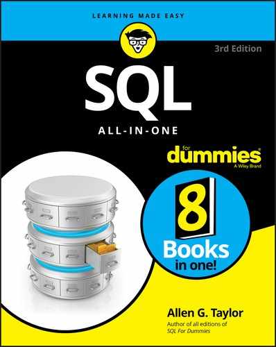
SELECT SalesOrderId, OrderDate, LastName, TotalDue
FROM Sales.SalesOrderHeader, Person.Person
WHERE BusinessEntityID = SalesPersonID
AND OrderDate >= '2011-05-01'
AND OrderDate < '2011-05-31'
You would receive a result similar to that shown in Figure 2-1. In this database, SalesOrderHeader is a table in the Sales schema and Person is a table in the Person schema. BusinessEntityID is the primary key of the SalesOrderHeader table, and SalesPersonID is the primary key of the Person table. SalesOrderID, OrderDate, and TotalDue are rows in the SalesOrderHeader table, and LastName is a row in the Person table.
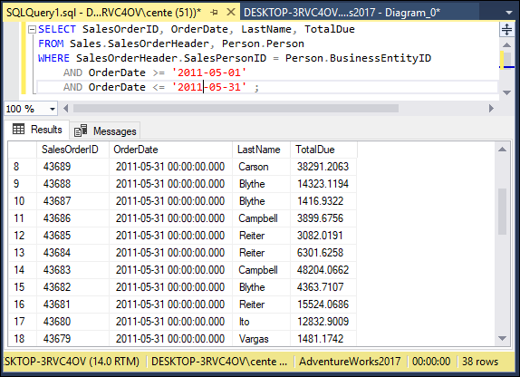
FIGURE 2-1: The result set for retrieval of sales for May 2011.
This result gives you some idea of how well your salespeople are doing because relatively few sales are involved. 38 rows were returned. However, in real life, a company would have many more sales, and it wouldn’t be as easy to tell whether sales objectives were being met. To do that, you can combine the GROUP BY clause with one of the aggregate functions (also called set functions) to get a quantitative picture of sales performance. For example, you can see which salesperson is selling more of the profitable high-ticket items by using the average (AVG) function as follows:
SELECT LastName, AVG(TotalDue)
FROM Sales.SalesOrderHeader, Person.Person
WHERE BusinessEntityID = SalesPersonID
AND OrderDate >= '2011-05-01'
AND OrderDate < '2011-05-31'
GROUP BY LastName;
You would receive a result similar to that shown in Figure 2-2. The GROUP BY clause causes records to be grouped by LastName and the groups to be sorted in ascending alphabetical order.
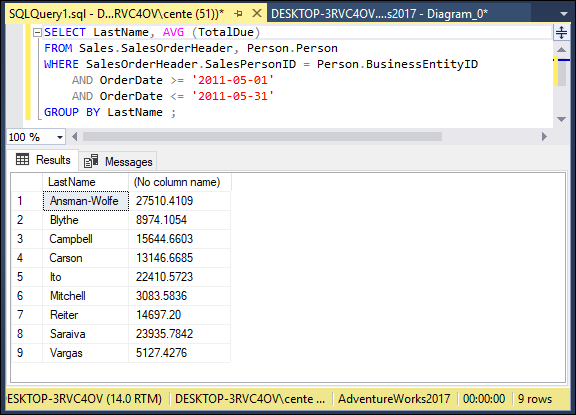
FIGURE 2-2: Average sales for each salesperson.
As shown in Figure 2-2, Ansman-Wolfe has the highest average sales. You can compare total sales with a similar query — this time using SUM:
SELECT LastName, SUM(TotalDue)
FROM Sales.SalesOrderHeader, Person.Person
WHERE BusinessEntityID = SalesPersonID
AND OrderDate >= '2011-05-01'
AND OrderDate < '2011-05-31'
GROUP BY LastName;
This gives the result shown in Figure 2-3. As in the previous example, the GROUP BY clause causes records to be grouped by LastName and the groups to be sorted in ascending alphabetical order.
FIGURE 2-3: Total sales for each salesperson.
Saraiva has the highest total sales for the month. Ansman-Wolfe has apparently sold only high-ticket items, but Saraiva has sold more across the entire product line.
HAVING clauses
You can analyze the grouped data further by using the HAVING clause. The HAVING clause is a filter that acts similar to a WHERE clause, but the filter acts on groups of rows rather than on individual rows. To illustrate the function of the HAVING clause, suppose Saraiva has just resigned, and the sales manager wants to display the overall data for the other salespeople. You can exclude Saraiva’s sales from the grouped data by using a HAVING clause as follows:
SELECT LastName, SUM(TotalDue)
FROM Sales.SalesOrderHeader, Person.Person
WHERE BusinessEntityID = SalesPersonID
AND OrderDate >= '2011-05-01'
AND OrderDate < '2011-05-31'
GROUP BY LastName
HAVING LastName <> 'Saraiva';
This gives the result shown in Figure 2-4. Only rows where the salesperson is not Saraiva are returned. As before, the GROUP BY clause causes records to be grouped by LastName and the groups to be sorted in ascending alphabetical order.
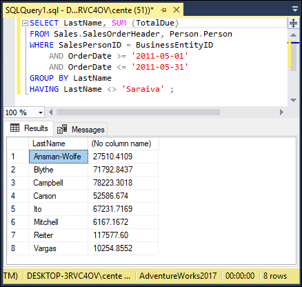
FIGURE 2-4: Total sales for all salespeople except Saraiva.
ORDER BY clauses
You can use the ORDER BY clause to display the output table of a query in either ascending or descending alphabetical order. Whereas the GROUP BY clause gathers rows into groups and sorts the groups into alphabetical order, ORDER BY sorts individual rows. The ORDER BY clause must be the last clause that you specify in a query. If the query also contains a GROUP BY clause, the clause first arranges the output rows into groups. The ORDER BY clause then sorts the rows within each group. If you have no GROUP BY clause, the statement considers the entire table as a group, and the ORDER BY clause sorts all its rows according to the column (or columns) that the ORDER BY clause specifies.
To illustrate this point, consider the data in the SalesOrderHeader table. The SalesOrderHeader table contains columns for SalesOrderID, OrderDate, DueDate, ShipDate, and SalesPersonID, among other things. If you use the following example, you see all the SALES data, but in an arbitrary order:
SELECT * FROM Sales.SalesOrderHeader ;
In one implementation, this order may be the one in which you inserted the rows in the table, and in another implementation, the order may be that of the most recent updates. The order can also change unexpectedly if anyone physically reorganizes the database. Usually, you want to specify the order in which you want to display the rows. You may, for example, want to see the rows in order by the OrderDate, as follows:
SELECT * FROM Sales.SalesOrderHeader ORDER BY OrderDate ;
This example returns all the rows in the SalesOrderHeader table, in ascending order by OrderDate.
For rows with the same OrderDate, the default order depends on the implementation. You can, however, specify how to sort the rows that share the same OrderDate. You may want to see the orders for each OrderDate in order by SalesOrderID, as follows:
SELECT * FROM Sales.SalesOrderHeader ORDER BY OrderDate, SalesOrderID ;
This example first orders the sales by OrderDate; then for each OrderDate, it orders the sales by SalesOrderID. But don’t confuse that example with the following query:
SELECT * FROM Sales.SalesOrderHeader ORDER BY SalesOrderID, OrderDate ;
This query first orders the sales by SalesOrderID. Then for each different SalesOrderID, the query orders the sales by OrderDate. This probably won’t yield the result you want because it is unlikely that multiple order dates exist for a single sales order number.
The following query is another example of how SQL can return data:
SELECT * FROM Sales.SalesOrderHeader ORDER BY SalesPersonID, OrderDate ;
This example first orders by salesperson and then by order date. After you look at the data in that order, you may want to invert it, as follows:
SELECT * FROM Sales.SalesPersonID ORDER BY OrderDate, SalesPersonID ;
This example orders the rows first by order date and then by salesperson.
All these ordering examples are ascending (ASC), which is the default sort order. In the AdventureWorks2017 sample database, this last SELECT would show earlier sales first and, within a given date, shows sales for 'Ansman-Wolfe' before 'Blythe'. If you prefer descending (DESC) order, you can specify this order for one or more of the order columns, as follows:
SELECT * FROM Sales.SalesPersonID ORDER BY OrderDate DESC, SalesPersonID ASC;
This example specifies a descending order for order date, showing the more recent orders first, and an ascending order for salespeople.
Tuning Queries
Performance is almost always a top priority for any organizational database system. As usage of the system goes up, if resources such as processor speed, cache memory, and hard disk storage do not go up proportionally, performance starts to suffer and users start to complain. Clearly, one thing that a system administrator can do is increase the resources — install a faster processor, add more cache, buy more hard disks. These solutions may give the needed improvement, and may even be necessary, but you should try a cheaper solution first: improving the efficiency of the queries that are loading down the system.
Generally, there are several different ways that you can obtain the information you want from a database; in other words, there are several different ways that you can code a query. Some of those ways are more efficient than others. If one or more queries that are run on a regular basis are bogging down the system, you may be able to bring your system back up to speed without spending a penny on additional hardware. You may just have to recode the queries that are causing the bottleneck.
Popular database management systems have query optimizers that try to eliminate bottlenecks for you, but they don’t always do as well as you could do if you tested various alternatives and picked the one with the best performance.
Unfortunately, no general rules apply across the board. The way a database is structured and the columns that are indexed have definite effects. In addition, a coding practice that would be optimal if you use Microsoft SQL Server might result in the worst possible performance if you use Oracle. Because the different DBMSs do things in different ways, what is good for one is not necessarily good for another. There are some things you can do, however, that enable you to find good query plans. In the following sections, I show you some common situations.
SELECT DISTINCT
You use SELECT DISTINCT when you want to make sure there are no duplicates in records you retrieve. However, the DISTINCT keyword potentially adds overhead to a query that could impact system performance. The impact it may or may not have depends on how it is implemented by the DBMS. Furthermore, including the DISTINCT keyword in a SELECT operation may not even be needed to ensure there are no duplicates. If you are doing a select on a primary key, the result set is guaranteed to contain no duplicates anyway, so adding the DISTINCT keyword provides no advantage.
Instead of relying on general rules such as, “Avoid using the DISTINCT keyword if you can,” if you suspect that a query that includes a DISTINCT keyword is inefficient, test it to see. First, make a typical query into Microsoft’s AdventureWorks2017 sample database. The AdventureWorks2017 database contains records typical of a commercial enterprise. There is a Customer table and a SalesOrderHeader table, among others. One thing you might want to do is see what companies in the Customer table have actually placed orders, as recorded in the Orders table. Because a customer may place multiple orders, it makes sense to use the DISTINCT keyword so that only one row is returned for each customer. Here’s the code for the query:
SELECT DISTINCT SalesOrderHeader.CustomerID, Customer.StoreID, SalesOrderHeader.TotalDue
FROM Sales.Customer, Sales.SalesOrderHeader
WHERE Customer.CustomerID = SalesOrderHeader.CustomerID ;
Before executing this query, click on the Include Client Statistics icon to select it. Then click the Execute button.
The result is shown in Figure 2-5, which shows the first few customer ID numbers of the 31,349 companies that have placed at least one order.
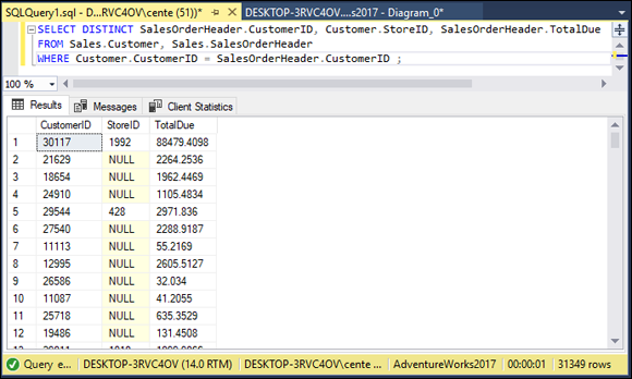
FIGURE 2-5: Customers who have placed at least one order.
In this query, I used CustomerID to link the Customer table to the SalesOrderHeader table so that I could pull information from both.
It would be interesting to see how efficient this query is. Use Microsoft SQL Server 2017’s tools to find out. First, look at the execution plan that was followed to run this query in Figure 2-6. To see the execution plan, click the Estimated Execution Plan icon in the toolbar.
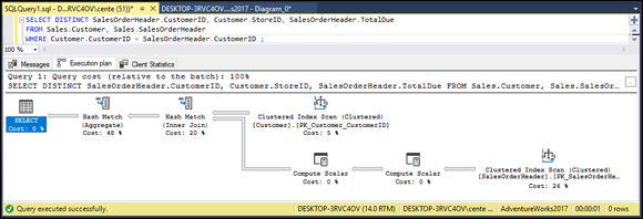
FIGURE 2-6: The SELECT DISTINCT query execution plan.
The execution plan shows that a hash match on an aggregation operation takes 48% of the execution time, and a hash match on an inner join takes another 20%. A clustered index scan on the primary key of the customer table takes 5% of the time, and a clustered index scan on the primary key of the SalesOrderHeader table takes 26%. To see how well or how poorly I’m doing, I look at the client statistics (Figure 2-7), by clicking the Include Client Statistics icon in the toolbar.
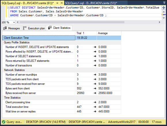
FIGURE 2-7: SELECT DISTINCT query client statistics.
I cover inner joins in Chapter 4 of this minibook. A clustered index scan is a row-by-row examination of the index on a table column. In this case, the index of SalesOrderHeader.CustomerID is scanned. The hash match on the aggregation operation and the hash match on the inner join are the operations used to match up the CustomerID from the Customer table with the CustomerID from the SalesOrderHeader table.
Total execution time is 447 time units, with client processing time at 2 time units and wait time on server replies at 445 time units.
The execution plan shows that the bulk of the time consumed is due to hash joins and clustered index scans. There is no getting around these operations, and it is doing it about as efficiently as possible.
Temporary tables
SQL is so feature-rich that there are multiple ways to perform many operations. Not all those ways are equally efficient. Often, the DBMS’s optimizer dynamically changes an operation that was coded in a suboptimal way into a more efficient operation. Sometimes, however, this doesn’t happen. To be sure your query is running as fast as possible, code it using a few different approaches and then test each approach. Settle on the one that does the best job. Sometimes the best method on one type of query performs poorly on another, so take nothing for granted.
One method of coding a query that has multiple selection conditions is to use temporary tables. Think of a temporary table as a scratchpad. You put some data in it as an intermediate step in an operation. When you are done with it, it disappears. Consider an example. Suppose you want to retrieve the last names of all the AdventureWorks employees whose first name is Janice. First you can create a temporary table that holds the information you want from the Person table in the Person schema:
SELECT PersonType, FirstName, LastName INTO #Temp
FROM Person.Person
WHERE PersonType = 'EM' ;
As you can see from the code, the result of the select operation is placed into a temporary table named #Temp rather than being displayed in a window. In SQL Server, local temporary tables are identified with a # sign as the first character.
Now you can find the Janices in the #Temp table:
SELECT FirstName, LastName
FROM #Temp
WHERE FirstName = 'Janice' ;
Running these two queries consecutively gives the result shown in Figure 2-8.

FIGURE 2-8: Retrieve all employees named Janice from the Person table.
The summary at the bottom of the screen shows that AdventureWorks has only one employee named Janice. Look at the execution plan (see Figure 2-9) to see how I did this retrieval.
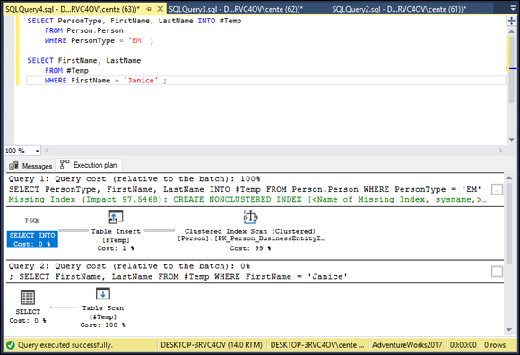
FIGURE 2-9: SELECT query execution plan using a temporary table.
Creation of the temporary table to separate the employees is one operation, and finding all the Janices is another. In the Table Creation query, creating the temporary table took up only 1% of the time used. A clustered index scan on the primary key of the Person table took up the other 99%. Also notice that a missing index was flagged, with an impact of over 97, followed by a recommendation to create a nonclustered index on the PersonType column. Considering the huge impact on runtime due to the absence of that index, if you were to run queries such as this frequently, you should consider creating an index on PersonType. Indexing PersonType in the Person table provides a big performance boost in this case because the number of employees in the table is a relatively small number out of over 31,000 total records.
The table scan of the temporary table took up all the time of the second query. How did you do performance-wise? Figure 2-10 gives the details from the Client Statistics tab.
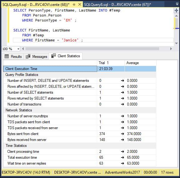
FIGURE 2-10: SELECT query execution client statistics using a temporary table.
As you see in the Client Statistics tab, total execution time was 65 time units, with two units going to client processing time and 63 units waiting for server replies. 374 bytes were sent from the client, and 148 bytes were returned by the server. These figures will vary from one run to the next due to caching and other factors.
Now suppose you performed the same operation without using a temporary table. You could do so with the following code:
SELECT FirstName, LastName
FROM Person.Person
WHERE PersonType = 'EM'
AND FirstName = 'Janice';
EM is AdventureWorks’ code for a PersonType of employee. You get the same result (shown in Figure 2-11) as in Figure 2-8. Janice Galvin is the only employee with a first name of Janice.
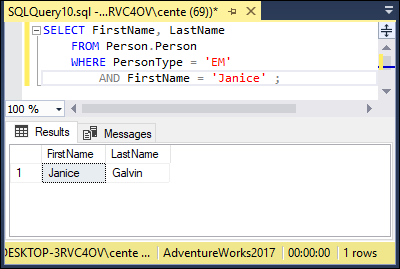
FIGURE 2-11: SELECT query result with a compound condition.
How does the execution plan (shown in Figure 2-12) compare with the one in Figure 2-9?
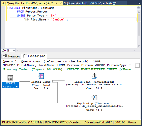
FIGURE 2-12: SELECT query execution plan with a compound condition.
As you can see, the same result was obtained by a completely different execution plan. A nonclustered index scan took up 77% of the total execution time, a key lookup took 15%, and the remaining 7% was consumed by an inner join. Once again, a recommendation for a nonclustered index has been made, this time on the combined PersonType and FirstName columns. The real story, however, is revealed in the client statistics (shown in Figure 2-13). How does performance compare with the temporary table version?
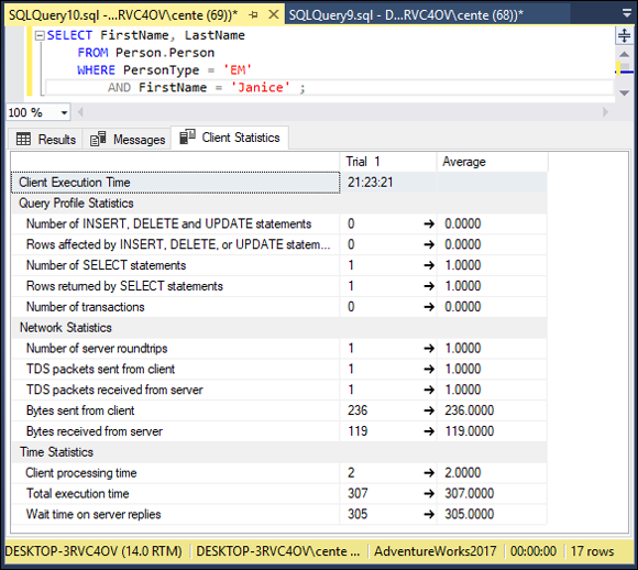
FIGURE 2-13: SELECT query client statistics, with a compound condition.
Hmmm. Total execution time is 307 time units, most of which is due to wait time for server replies. That’s more than the 65 time units consumed by the temporary table formulation. 236 bytes were sent from the client, which is significantly less than the upstream traffic in the temporary table case. In addition, only 119 bytes were sent from the server down to the client. That’s comparable to the 148 bytes that were downloaded using the temporary table. All things considered, the performance of both methods turns out to be about a wash. There may be situations where using one or the other is better, but creating a nonclustered index on [PersonType] in the first case, or on [PersonType, FirstName] in the second case will have a much bigger impact.
The ORDER BY clause
The ORDER BY clause can be expensive in terms of both bandwidth between the server and the client and execution time simply because ORDER BY initiates a sort operation, and sorts consume large amounts of both time and memory. If you can minimize the number of ORDER BY clauses in a series of queries, you may save resources. This is one place where using a temporary table might perform better. Consider an example. Suppose you want to do a series of retrievals on your Products table, in which you see which products are available in several price ranges. For example, you want one list of products priced between 10 dollars and 20 dollars, ordered by unit price. Then you want a list of products priced between 20 dollars and 30 dollars, similarly ordered, and so on. To cover four such price ranges, you could make four queries, all four with an ORDER BY clause. Alternatively, you could create a temporary table with a query that uses an ORDER BY clause, and then draw the data for the ranges in separate queries that do not have ORDER BY clauses. Compare the two approaches. Here’s the code for the temporary table approach:
SELECT Name, ListPrice INTO #Product
FROM Production.Product
WHERE ListPrice > 10
AND ListPrice <= 50
ORDER BY ListPrice;
SELECT Name, ListPrice
FROM #Product
WHERE ListPrice > 10
AND ListPrice <= 20;
SELECT Name, ListPrice
FROM #Product
WHERE ListPrice > 20
AND ListPrice <= 30;
SELECT Name, ListPrice
FROM #Product
WHERE ListPrice > 30
AND ListPrice <= 40;
SELECT Name, ListPrice
FROM #Product
WHERE ListPrice > 40
AND ListPrice <= 50;
The execution plan for this series of queries is shown in Figure 2-14.
FIGURE 2-14: Execution plan, minimizing occurrence of ORDER BY clauses.
The first query, the one that creates the temporary table, has the most complex execution plan. By itself, it takes up 64% of the allotted time, and the other four queries take up the remaining 36%. Figure 2-15 shows the client statistics, measuring resource usage.

FIGURE 2-15: Client statistics, minimizing occurrence of ORDER BY clauses.
Total execution time varies from run to run because of variances in the time spent waiting to hear back from the server, and an average of 13,175 bytes were received from the server. Now compare that with no temporary table, but four separate queries, each with its own ORDER BY clause. Here’s the code:
SELECT Name, ListPrice
FROM #Product
WHERE ListPrice > 10
AND ListPrice <= 20
ORDER BY ListPrice ;
SELECT Name, ListPrice
FROM #Product
WHERE ListPrice > 20
AND ListPrice <= 30
ORDER BY ListPrice ;
SELECT Name, ListPrice
FROM #Product
WHERE ListPrice > 30
AND ListPrice <= 40
ORDER BY ListPrice ;
SELECT Name, ListPrice
FROM #Product
WHERE ListPrice > 40
AND ListPrice <= 50
ORDER BY ListPrice ;
The resulting execution plan is shown in Figure 2-16.

FIGURE 2-16: Execution plan, queries with separate ORDER BY clauses.
Each of the four queries involves a sort, which consumes 48% of the total time of the query. This could be costly. Figure 2-17 shows what the client statistics look like.

FIGURE 2-17: Client statistics, queries with separate ORDER BY clauses.
Total execution time varies from one run to the next, primarily due to waiting for a response from the server. The number of bytes returned by the server also varies. A cursory look at the statistics does not determine whether this latter method is slower than the temporary table method; averages over multiple independent runs will be required. At any rate, as table sizes increase, the time it takes to sort them goes up exponentially. For larger tables, the performance advantage tips strongly to the temporary table method.
The HAVING clause
Think about the order in which you do things. Performing operations in the correct order can make a big difference in how long it takes to complete those operations. Whereas the WHERE clause filters out rows that don’t meet a search condition, the HAVING clause filters out entire groups that don’t meet a search condition. It makes sense to filter first (with a WHERE clause) and group later (with a GROUP BY clause) rather than group first and filter later (with a HAVING clause). If you group first, you perform the grouping operation on everything. If you filter first, you perform the grouping operation only on what is left after the rows you don’t want have been filtered out.
This line of reasoning sounds good. To see if it is borne out in practice, consider this code:
SELECT AVG(ListPrice) AS AvgPrice, ProductLine
FROM Production.Product
GROUP BY ProductLine
HAVING ProductLine = 'T' ;
It finds the average price of all the products in the T product line by first grouping the products into categories and then filtering out all except those in product line T. The AS keyword is used to give a name to the average list price — in this case the name is AvgPrice. Figure 2-18 shows what SQL Server returns. This formulation should result in worse performance than filtering first and grouping second.
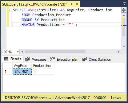
FIGURE 2-18: Retrieval with a HAVING clause.
The average price for the products in product line T is $840.7621. Figure 2-19 shows what the execution plan tells us.
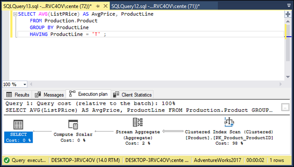
FIGURE 2-19: Retrieval with a HAVING clause execution plan.
A clustered index scan takes up most of the time. This is a fairly efficient operation. The client statistics are shown in Figure 2-20.
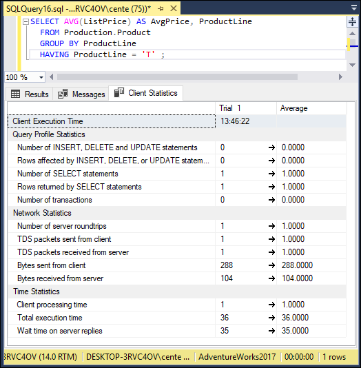
FIGURE 2-20: Retrieval with a HAVING clause client statistics.
Client execution time is about 13 time units. Now, try filtering first and grouping second.
SELECT AVG(ListPrice) AS AvgPrice
FROM Production.Product
WHERE ProductLine = 'T' ;
There is no need to group because all product lines except product line T are filtered out by the WHERE clause. Figure 2-21 shows that the result is the same as in the previous case, $840.7621.
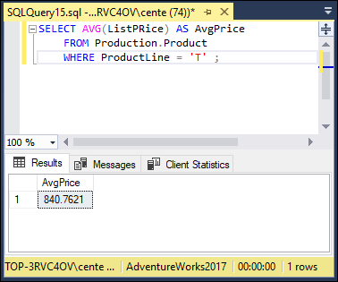
FIGURE 2-21: Retrieval without a HAVING clause.
Figure 2-22 shows how the execution plan differs.
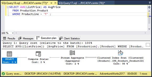
FIGURE 2-22: Retrieval without a HAVING clause execution plan.
Interesting! The execution plan is exactly the same. SQL Server’s optimizer has done its job and optimized the less efficient case. Are the client statistics the same too? Check Figure 2-23 to find out.
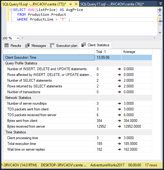
FIGURE 2-23: Retrieval without a HAVING clause client statistics.
Client execution time is essentially the same.
The OR logical connective
Some systems never use indexes when expressions in a WHERE clause are connected by the OR logical connective. Check your system to see if it does. See how SQL Server handles it.
SELECT ProductID, Name
FROM Production.Product
WHERE ListPrice < 20
OR SafetyStockLevel < 30 ;
Check the execution plan to see if SQL Server uses an index (like the one shown in Figure 2-24). SQL Server does use an index in this situation, so there is no point in looking for alternative ways to code this type of query.
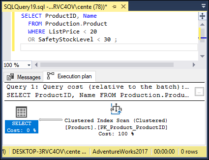
FIGURE 2-24: Query with an OR logical connective.
Run performance tests such as those shown in this chapter on the exact database you are attempting to tune, rather than on a sample database such as AdventureWorks2017, or even on another production database. Due to differences in table size, indexing, and other factors, conclusions you come to, based on one database, don’t necessarily apply to another.