Chapter 3
Querying Multiple Tables with Subqueries
IN THIS CHAPTER
![]() Defining subqueries
Defining subqueries
![]() Discovering how subqueries work
Discovering how subqueries work
![]() Nesting subqueries
Nesting subqueries
![]() Tuning nested subqueries
Tuning nested subqueries
![]() Tuning correlation subqueries
Tuning correlation subqueries
Relational databases have multiple tables. That’s where the word relational comes from — multiple tables that relate to each other in some way. One consequence of the distribution of data across multiple tables is that most queries need to pull data from more than one of them. There are a couple of ways to do this. One is to use relational operators, which I cover in the next chapter. The other method is to use subqueries, which is the subject of this chapter.
What Is a Subquery?
A subquery is an SQL statement embedded within another SQL statement. It’s possible for a subquery to be embedded within another subquery, which is in turn embedded within an outermost SQL statement. Theoretically, there is no limit to the number of levels of subquery that an SQL statement may include, although any given implementation has a practical limit. A key feature of a subquery is that the table or tables that it references need not be the same as the table or tables referenced by its enclosing query. This has the effect of returning results based on the information in multiple tables.
What Subqueries Do
Subqueries are located within the WHERE clause of their enclosing statement. Their function is to set the search conditions for the WHERE clause. The combination of a subquery and its enclosing query is called a nested query. Different kinds of nested queries produce different results. Some subqueries produce a list of values that is then used as input by the enclosing statement. Other subqueries produce a single value that the enclosing statement then evaluates with a comparison operator. A third kind of subquery, called a correlated subquery, operates differently, and I discuss it in the upcoming “Correlated subqueries” section.
Subqueries that return multiple values
A key concern of many businesses is inventory control. When you are building products that are made up of various parts, you want to make sure that you have an adequate supply of all the parts. If just one part is in short supply, it could bring the entire manufacturing operation to a screeching halt. To see how many products are impacted by the lack of a part they need, you can use a subquery.
Subqueries that retrieve rows satisfying a condition
Suppose your company (Penguin Electronics, Inc.) manufactures a variety of electronic products, such as audio amplifiers, FM radio tuners, and handheld metal detectors. You keep track of inventory of all your products — as well as all the parts that go into their manufacture — in a relational database. The database has a PRODUCTS table that holds the inventory levels of finished products and a PARTS table that holds the inventory levels of the parts that go into the products.
A part could be included in multiple products, and each product is made up of multiple parts. This means that there is a many-to-many relationship between the PRODUCTS table and the PARTS table. Because this could present problems (see Book 2, Chapter 3 for a rundown of the kinds of problems I mean), you decide to insert an intersection table between PRODUCTS and PARTS, transforming the problematical many-to-many relationship into two easier-to-deal-with one-to-many relationships. The intersection table, named PROD_PARTS, takes the primary keys of PRODUCTS and PARTS as its only attributes. You can create these three tables with the following code:
CREATE TABLE PRODUCTS (
ProductID INTEGER PRIMARY KEY,
ProductName CHAR (30),
ProductDescription CHAR (50),
ListPrice NUMERIC (9,2),
QuantityInStock INTEGER ) ;
CREATE TABLE PARTS (
PartID INTEGER PRIMARY KEY,
PartName CHAR (30),
PartDescription CHAR (50),
QuantityInStock INTEGER ) ;
CREATE TABLE PROD_PARTS (
ProductID INTEGER NOT NULL,
PartID INTEGER NOT NULL ) ;
Suppose some of your products include an APM-17 DC analog panel meter. Now you find to your horror that you are completely out of the APM-17 part. You can’t complete the manufacture of any product that includes it. It is time for management to take some emergency actions. One is to check on the status of any outstanding orders to the supplier of the APM-17 panel meters. Another is to notify the sales department to stop selling all products that include the APM-17, and switch to promoting products that do not include it.
To discover which products include the APM-17, you can use a nested query such as the following:
SELECT ProductID
FROM PROD_PARTS
WHERE PartID IN
(SELECT PartID
FROM PARTS
WHERE PartDescription = 'APM-17') ;
SQL processes the innermost query first, so it queries the PARTS table, returning the PartID of every row in the PARTS table where the PartDescription is APM-17. There should be only one such row. Only one part should have a description of APM-17. The outer query uses the IN keyword to find all the rows in the PROD_PARTS table that include the PartID that appears in the result set from the inner query. The outer query then extracts from the PROD_PARTS table the ProductIDs of all the products that include the APM-17 part. These are the products that the Sales department should stop selling.
Subqueries that retrieve rows that don’t satisfy a condition
Because sales are the lifeblood of any business, it is even more important to determine which products the Sales team can continue to sell than it is to tell them what not to sell. You can do this with another nested query. Use the query just executed in the preceding section as a base, add one more layer of query to it, and return the ProductIDs of all the products not affected by the APM-17 shortage.
SELECT ProductID
FROM PROD_PARTS
WHERE ProductID NOT IN
(SELECT ProductID
FROM PROD_PARTS
WHERE PartID IN
(SELECT PartID
FROM PARTS
WHERE PartDescription = 'APM-17') ;
The two inner queries return the ProductIDs of all the products that include the APM-17 part. The outer query returns all the ProductIDs of all the products that are not included in the result set from the inner queries. This final result set is the list of ProductIDs of products that do not include the APM-17 analog panel meter.
Subqueries that return a single value
Introducing a subquery with one of the six comparison operators (=, <>, <, <=, >, >=) is often useful. In such a case, the expression preceding the operator evaluates to a single value, and the subquery following the operator must also evaluate to a single value. An exception is the case of the quantified comparison operator, which is a comparison operator followed by a quantifier (ANY, SOME, or ALL).
To illustrate a case in which a subquery returns a single value, look at another piece of Penguin Electronics’ database. It contains a CUSTOMER table that holds information about the companies that buy Penguin products. It also contains a CONTACT table that holds personal data about individuals at each of Penguin’s customer organizations. The following code creates Penguin’s CUSTOMER and CONTACT tables.
CREATE TABLE CUSTOMER (
CustomerID INTEGER PRIMARY KEY,
Company CHAR (40),
Address1 CHAR (50),
Address2 CHAR (50),
City CHAR (25),
State CHAR (2),
PostalCode CHAR (10),
Phone CHAR (13) ) ;
CREATE TABLE CONTACT (
CustomerID INTEGER PRIMARY KEY,
FirstName CHAR (15),
LastName CHAR (20),
Phone CHAR (13),
Email CHAR (30),
Fax CHAR (13),
Notes CHAR (100),
CONSTRAINT ContactFK FOREIGN KEY (CustomerID)
REFERENCES CUSTOMER (CustomerID) ) ;
Say that you want to look at the contact information for the customer named Baker Electronic Sales, but you don’t remember that company’s CustomerID. Use a nested query like this one to recover the information you want:
SELECT *
FROM CONTACT
WHERE CustomerID =
(SELECT CustomerID
FROM CUSTOMER
WHERE Company = 'Baker Electronic Sales') ;
The result looks something like this:
CustomerID FirstName LastName Phone Notes
---------- --------- -------- ------------ --------------
787 David Lee 555-876-3456 Likes to visit
El Pollo Loco
when in Cali.
You can now call Dave at Baker and tell him about this month’s special sale on metal detectors.
When you use a subquery in an "=" comparison, the subquery’s SELECT list must specify a single column (CustomerID in the example). When the subquery is executed, it must return a single row in order to have a single value for the comparison.
In this example, I assume that the CUSTOMER table has only one row with a Company value of Baker Electronic Sales. If the CREATE TABLE statement for CUSTOMER specified a UNIQUE constraint for Company, such a statement guarantees that the subquery in the preceding example returns a single value (or no value). Subqueries like the one in the example, however, are commonly used on columns not specified to be UNIQUE. In such cases, you are relying on some other reasons for believing that the column has no duplicates.
If more than one CUSTOMER has a value of Baker Electronic Sales in the Company column (perhaps in different states), the subquery raises an error.
If no Customer with such a company name exists, the subquery is treated as if it were null, and the comparison becomes unknown. In this case, the WHERE clause returns no row (because it returns only rows with the condition True and filters rows with the condition False or Unknown). This would probably happen, for example, if someone misspelled the COMPANY as Baker Electronics Sales.
Although the equals operator (=) is the most common, you can use any of the other five comparison operators in a similar structure. For every row in the table specified in the enclosing statement’s FROM clause, the single value returned by the subquery is compared to the expression in the enclosing statement’s WHERE clause. If the comparison gives a True value, a row is added to the result table.
You can guarantee that a subquery returns a single value if you include a set function in it. Set functions, also known as aggregate functions, always return a single value. (I describe set functions in Chapter 1 of this minibook.) Of course, this way of returning a single value is helpful only if you want the result of a set function.
Say that you are a Penguin Electronics salesperson and you need to earn a big commission check to pay for some unexpected bills. You decide to concentrate on selling Penguin’s most expensive product. You can find out what that product is with a nested query:
SELECT ProductID, ProductName, ListPrice
FROM PRODUCT
WHERE ListPrice =
(SELECT MAX(ListPrice)
FROM PRODUCT) ;
This is an example of a nested query where both the subquery and the enclosing statement operate on the same table. The subquery returns a single value: the maximum list price in the PRODUCTS table. The outer query retrieves all rows from the PRODUCTS table that have that list price.
The next example shows a comparison subquery that uses a comparison operator other than =:
SELECT ProductID, ProductName, ListPrice
FROM PRODUCTS
WHERE ListPrice <
(SELECT AVG(ListPrice)
FROM PRODUCTS) ;
The subquery returns a single value: the average list price in the PRODUCTS table. The outer query retrieves all rows from the PRODUCTS table that have a list price less than the average list price.
 In the original SQL standard, a comparison could have only one subquery, and it had to be on the right side of the comparison. SQL:1999 allowed either or both operands of the comparison to be subqueries, and later versions of SQL retain that expanded capability.
Quantified subqueries return a single value
One way to make sure a subquery returns a single value is to introduce it with a quantified comparison operator. The universal quantifier ALL, and the existential quantifiers SOME and ANY, when combined with a comparison operator, process the result set returned by the inner subquery, reducing it to a single value.
Look at an example. From the 1960s through the 1980s, there was fierce competition between Ford and Chevrolet to produce the most powerful cars. Both companies had small-block V-8 engines that went into Mustangs, Camaros, and other performance-oriented vehicles.
Power is measured in units of horsepower. In general, a larger engine delivers more horsepower, all other things being equal. Because the displacements (sizes) of the engines varied from one model to another, it’s unfair to look only at horsepower. A better measure of the efficiency of an engine is horsepower per displacement. Displacement is measured in cubic inches (CID). Table 3-1 shows the year, displacement, and horsepower ratings for Ford small-block V-8s between 1960 and 1980.
TABLE 3-1 Ford Small-Block V-8s, 1960–1980
Year |
Displacement (CID) |
Maximum Horsepower |
Notes |
1962 |
221 |
145 |
|
1963 |
289 |
225 |
4bbl carburetor |
1965 |
289 |
271 |
289HP model |
1965 |
289 |
306 |
Shelby GT350 |
1969 |
351 |
290 |
4bbl carburetor |
1975 |
302 |
140 |
Emission regulations |
The Shelby GT350 was a classic muscle car — not a typical car for the weekday commute. Emission regulations taking effect in the early 1970s halved power output and brought an end to the muscle car era. Table 3-2 shows what Chevy put out during the same timeframe.
TABLE 3-2 Chevy Small-Block V-8s, 1960–1980
Year |
Displacement (CID) |
Maximum Horsepower |
Notes |
1960 |
283 |
315 |
|
1962 |
327 |
375 |
|
1967 |
350 |
295 |
|
1968 |
302 |
290 |
|
1968 |
307 |
200 |
|
1969 |
350 |
370 |
Corvette |
1970 |
400 |
265 |
|
1975 |
262 |
110 |
Emission regulations |
Here again you see the effect of the emission regulations that kicked in circa 1971 — a drastic drop in horsepower per displacement.
Use the following code to create tables to hold these data items:
CREATE TABLE Ford (
EngineID INTEGER PRIMARY KEY,
ModelYear CHAR (4),
Displacement NUMERIC (5,2),
MaxHP NUMERIC (5,2),
Notes CHAR (30) ) ;
CREATE TABLE Chevy (
EngineID INTEGER PRIMARY KEY,
ModelYear CHAR (4),
Displacement NUMERIC (5,2),
MaxHP NUMERIC (5,2),
Notes CHAR (30) ) ;
After filling these tables with the data in Tables 3-1 and 3-2, you can run some queries. Suppose you are a dyed-in-the-wool Chevy fan and are quite certain that the most powerful Chevrolet has a higher horsepower-to-displacement ratio than any of the Fords. To verify that assumption, enter the following query:
SELECT *
FROM Chevy
WHERE (MaxHP/Displacement) > ALL
(SELECT (MaxHP/Displacement) FROM Ford) ;
This returns the result shown in Figure 3-1:
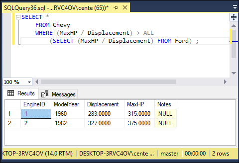
FIGURE 3-1: Chevy muscle cars with horsepower to displacement ratios higher than any of the Fords listed.
The subquery (SELECT (MaxHP/Displacement) FROM Ford) returns the horsepower-to-displacement ratios of all the Ford engines in the Ford table. The ALL quantifier says to return only those records from the Chevy table that have horsepower-to-displacement ratios higher than all the ratios returned for the Ford engines. Two different Chevy engines had higher ratios than any Ford engine of that era, including the highly regarded Shelby GT350. Ford fans should not be bothered by this result, however. There’s more to what makes a car awesome than just the horsepower-to-displacement ratio.
What if you had made the opposite assumption? What if you had entered the following query?
SELECT *
FROM Ford
WHERE (MaxHP/Displacement) > ALL
(SELECT (MaxHP/Displacement) FROM Chevy) ;
Because none of the Ford engines has a higher horsepower-to-displacement ratio than all of the Chevy engines, the query doesn’t return any rows.
Correlated subqueries
In all the nested queries I show in the previous sections, the inner subquery is executed first, and then its result is applied to the outer enclosing statement. A correlated subquery first finds the table and row specified by the enclosing statement, and then executes the subquery on the row in the subquery’s table that correlates with the current row of the enclosing statement’s table.
Using a subquery as an existence test
Subqueries introduced with the EXISTS or the NOT EXISTS keyword are examples of correlated subqueries. The subquery either returns one or more rows, or it returns none. If it returns at least one row, the EXISTS predicate succeeds, and the enclosing statement performs its action. In the same circumstances, the NOT EXISTS predicate fails, and the enclosing statement does not perform its action. After one row of the enclosing statement’s table is processed, the same operation is performed on the next row. This action is repeated until every row in the enclosing statement’s table has been processed.
TESTING FOR EXISTENCE
Say that you are a salesperson for Penguin Electronics and you want to call your primary contact people at all of Penguin’s customer organizations in New Hampshire. Try the following query:
SELECT *
FROM CONTACT
WHERE EXISTS
(SELECT *
FROM CUSTOMER
WHERE State = 'NH'
AND CONTACT.CustomerID = CUSTOMER.CustomerID) ;
Notice the reference to CONTACT.CustomerID, which is referencing a column from the outer query and comparing it with another column, CUSTOMER.CustomerID, from the inner query. For each candidate row of the outer query, you evaluate the inner query, using the CustomerID value from the current CONTACT row of the outer query in the WHERE clause of the inner query.
The CustomerID column links the CONTACT table to the CUSTOMER table. SQL looks at the first record in the CONTACT table, finds the row in the CUSTOMER table that has the same CustomerID, and checks that row’s State field. If CUSTOMER.State = 'NH', the current CONTACT row is added to the result table. The next CONTACT record is then processed in the same way, and so on, until the entire CONTACT table has been processed. Because the query specifies SELECT * FROM CONTACT, all the CONTACT table’s fields are returned, including the contact’s name and phone number.
TESTING FOR NONEXISTENCE
In the previous example, the Penguin salesperson wants to know the names and numbers of the contact people of all the customers in New Hampshire. Imagine that a second salesperson is responsible for all of the United States except New Hampshire. She can retrieve her contacts by using NOT EXISTS in a query similar to the preceding one:
SELECT *
FROM CONTACT
WHERE NOT EXISTS
(SELECT *
FROM CUSTOMER
WHERE State = 'NH'
AND CONTACT.CustomerID = CUSTOMER.CustomerID) ;
Every row in CONTACT for which the subquery does not return a row is added to the result table.
Introducing a correlated subquery with the IN keyword
As I note in a previous section of this chapter, subqueries introduced by IN or by a comparison operator need not be correlated queries, but they can be. In the “Subqueries that retrieve rows satisfying a condition” section, I give examples of how a noncorrelated subquery can be used with the IN predicate. To show how a correlated subquery may use the IN predicate, ask the same question that came up with the EXISTS predicate: What are the names and phone numbers of the contacts at all of Penguin’s customers in New Hampshire? You can answer this question with a correlated IN subquery:
SELECT *
FROM CONTACT
WHERE 'NH' IN
(SELECT State
FROM CUSTOMER
WHERE CONTACT.CustomerID = CUSTOMER.CustomerID) ;
The statement is evaluated for each record in the CONTACT table. If, for that record, the CustomerID numbers in CONTACT and CUSTOMER match, the value of CUSTOMER.State is compared to 'NH'. The result of the subquery is a list that contains, at most, one element. If that one element is 'NH', the WHERE clause of the enclosing statement is satisfied, and a row is added to the query’s result table.
Introducing a correlated subquery with a comparison operator
A correlated subquery can also be introduced by one of the six comparison operators, as shown in the next example.
Penguin pays bonuses to its salespeople based on their total monthly sales volume. The higher the volume, the higher the bonus percentage. The bonus percentage list is kept in the BONUSRATE table:
MinAmount MaxAmount BonusPct
--------- --------- --------
0.00 24999.99 0.
25000.00 49999.99 0.01
50000.00 99999.99 0.02
100000.00 249999.99 0.03
250000.00 499999.99 0.04
500000.00 749999.99 0.05
750000.00 999999.99 0.06
If a person’s monthly sales total is between $100,000.00 and $249,999.99, the bonus is 3 percent of sales.
Sales are recorded in a transaction master table named TRANSMASTER, which is created as follows:
CREATE TABLE TRANSMASTER (
TransID INTEGER PRIMARY KEY,
CustID INTEGER FOREIGN KEY,
EmpID INTEGER FOREIGN KEY,
TransDate DATE,
NetAmount NUMERIC,
Freight NUMERIC,
Tax NUMERIC,
InvoiceTotal NUMERIC) ;
Sales bonuses are based on the sum of the NetAmount field for all of a person’s transactions in the month. You can find any person’s bonus rate with a correlated subquery that uses comparison operators:
SELECT BonusPct
FROM BONUSRATE
WHERE MinAmount <=
(SELECT SUM(NetAmount)
FROM TRANSMASTER
WHERE EmpID = 133)
AND MaxAmount >=
(SELECT SUM(NetAmount)
FROM TRANSMASTER
WHERE EmpID = 133) ;
This query is interesting in that it contains two subqueries, making use of the logical connective AND. The subqueries use the SUM aggregate operator, which returns a single value: the total monthly sales of employee 133. That value is then compared against the MinAmount and the MaxAmount columns in the BONUSRATE table, producing the bonus rate for that employee.
If you had not known the EmpID but had known the person’s name, you could arrive at the same answer with a more complex query:
SELECT BonusPct
FROM BONUSRATE
WHERE MinAmount <=
(SELECT SUM(NetAmount)
FROM TRANSMASTER
WHERE EmpID =
(SELECT EmployeeID
FROM EMPLOYEE
WHERE EmplName = 'Thornton'))
AND MaxAmount >=
(SELECT SUM(NetAmount)
FROM TRANSMASTER
WHERE EmpID =
(SELECT EmployeeID
FROM EMPLOYEE
WHERE EmplName = 'Thornton'));
This example uses subqueries nested within subqueries, which in turn are nested within an enclosing query, to arrive at the bonus rate for the employee named Thornton. This structure works only if you know for sure that the company has one, and only one, employee whose name is Thornton. If you know that more than one employee is named Thornton, you can add terms to the WHERE clause of the innermost subquery until you’re sure that only one row of the EMPLOYEE table is selected.
Correlated subqueries in a HAVING clause
You can have a correlated subquery in a HAVING clause just as you can in a WHERE clause. As I mention in Chapter 2 of this minibook, a HAVING clause is normally preceded by a GROUP BY clause. The HAVING clause acts as a filter to restrict the groups created by the GROUP BY clause. Groups that don’t satisfy the condition of the HAVING clause are not included in the result. When used in this way, the HAVING clause is evaluated for each group created by the GROUP BY clause. In the absence of a GROUP BY clause, the HAVING clause is evaluated for the set of rows passed by the WHERE clause, which is considered to be a single group. If neither a WHERE clause nor a GROUP BY clause is present, the HAVING clause is evaluated for the entire table:
SELECT TM1.EmpID
FROM TRANSMASTER TM1
GROUP BY TM1.EmpID
HAVING MAX(TM1.NetAmount) >= ALL
(SELECT 2 * AVG (TM2.NetAmount)
FROM TRANSMASTER TM2
WHERE TM1.EmpID <> TM2.EmpID) ;
This query uses two aliases for the same table, enabling you to retrieve the EmpID number of all salespeople who had a sale of at least twice the average value of all the other salespeople. Short aliases such as TM1 are often used to eliminate excessive typing when long table names such as TRANSMASTER are involved. But in this case, aliases do more than just save some typing. The TRANSMASTER table is used for two different purposes, so two different aliases are used to distinguish between them. The query works as follows:
- The outer query groups TRANSMASTER rows by the EmpID. This is done with the
SELECT,FROM, andGROUP BYclauses. - The
HAVINGclause filters these groups. For each group, it calculates theMAXof the NetAmount column for the rows in that group. - The inner query evaluates twice the average
NetAmountfrom all rows of TRANSMASTER whoseEmpIDis different from theEmpIDof the current group of the outer query. Each group contains the transaction records for an employee whose biggest sale had at least twice the value of the average of the sales of all the other employees. Note that in the last line, you need to reference two different EmpID values, so in theFROMclauses of the outer and inner queries, you use different aliases for TRANSMASTER. - You then use those aliases in the comparison of the query’s last line to indicate that you’re referencing both the
EmpIDfrom the current row of the inner subquery (TM2.EmpID) and theEmpIDfrom the current group of the outer subquery (TM1.EmpID).
Using Subqueries in INSERT, DELETE, and UPDATE Statements
In addition to SELECT statements, UPDATE, DELETE, and INSERT statements can also include WHERE clauses. Those WHERE clauses can contain subqueries in the same way that SELECT statement WHERE clauses do.
For example, Penguin has just made a volume purchase deal with Baker Electronic Sales and wants to retroactively provide Baker with a 10 percent credit for all its purchases in the last month. You can give this credit with an UPDATE statement:
UPDATE TRANSMASTER
SET NetAmount = NetAmount * 0.9
WHERE CustID =
(SELECT CustID
FROM CUSTOMER
WHERE Company = 'Baker Electronic Sales') ;
You can also have a correlated subquery in an UPDATE statement. Suppose the CUSTOMER table has a column LastMonthsMax, and Penguin wants to give the same 10 percent credit for purchases that exceed LastMonthsMax for the customer:
UPDATE TRANSMASTER TM
SET NetAmount = NetAmount * 0.9
WHERE NetAmount >
(SELECT LastMonthsMax
FROM CUSTOMER C
WHERE C.CustID = TM.CustID) ;
Note that this subquery is correlated: The WHERE clause in the last line references both the CustID of the CUSTOMER row from the subquery and the CustID of the current TRANSMASTER row that is a candidate for updating.
A subquery in an UPDATE statement can also reference the table being updated. Suppose that Penguin wants to give a 10 percent credit to customers whose purchases have exceeded $10,000:
UPDATE TRANSMASTER TM1
SET NetAmount = NetAmount * 0.9
WHERE 10000 < (SELECT SUM(NetAmount)
FROM TRANSMASTER TM2
WHERE TM1.CustID = TM2.CustID);
The inner subquery calculates the SUM of the NetAmount column for all TRANSMASTER rows for the same customer. What does this mean? Suppose that the customer with CustID = 37 has four rows in TRANSMASTER with values for NetAmount: 3000, 5000, 2000, and 1000. The SUM of NetAmount for this CustID is 11000.
 The order in which the
 UPDATE statement processes the rows is defined by your implementation and is generally not predictable. The order may differ depending on how the rows are arranged on the disk. Assume that the implementation processes the rows for this CustID in this order: first the TRANSMASTER row with a NetAmount of 3000, and then the one with NetAmount = 5000, and so on. After the first three rows for CustID 37 have been updated, their NetAmount values are 2700 (90 percent of 3000), 4500 (90 percent of 5000), and 1800 (90 percent of 2000). Then when you process the last TRANSMASTER row for CustID 37, whose NetAmount is 1000, the SUM returned by the subquery would seem to be 10000 — that is, the SUM of the new NetAmount values of the first three rows for CustID 37 and the old NetAmount value of the last row for CustID 37. Thus it would seem that the last row for CustID 37 isn’t updated because the comparison with that SUM is not True, since 10000 is not less than SELECT SUM (NetAmount). But that is not how the UPDATE statement is defined when a subquery references the table being updated. All evaluations of subqueries in an UPDATE statement reference the old values of the table being updated. In the preceding UPDATE for CustID 37, the subquery returns 11000 — the original SUM.
The subquery in an UPDATE statement WHERE clause operates the same as it does in a SELECT statement WHERE clause. The same is true for DELETE and INSERT. To delete all of Baker’s transactions, use this statement:
DELETE FROM TRANSMASTER
WHERE CustID =
(SELECT CustomerID
FROM CUSTOMER
WHERE Company = 'Baker Electronic Sales') ;
As with UPDATE, DELETE subqueries can also be correlated and can also reference the table whose rows are being deleted. The rules are similar to the rules for UPDATE subqueries. Suppose you want to delete all rows from TRANSMASTER for customers whose total NetAmount is larger than $10,000:
DELETE FROM TRANSMASTER TM1
WHERE 10000 < (SELECT SUM(NetAmount)
FROM TRANSMASTER TM2
WHERE TM1.CustID = TM2.CustID) ;
This query deletes all rows from TRANSMASTER referencing customers with purchases exceeding $10,000 — including the aforementioned customer with CustID 37. All references to TRANSMASTER in the subquery denote the contents of TRANSMASTER before any deletes by the current statement. So even when you are deleting the last TRANSMASTER row, the subquery is evaluated on the original TRANSMASTER table, identified by TM1.
When you update, delete, or insert database records, you risk making a table’s data inconsistent with other tables in the database. Such an inconsistency is called a modification anomaly, discussed in Book 2, Chapter 2. If you delete TRANSMASTER records and a TRANSDETAIL table depends on TRANSMASTER, you must delete the corresponding records from TRANSDETAIL too. This operation is called a cascading delete because the deletion of a parent record cascades to its associated child records. Otherwise, the undeleted child records become orphans. In this case, they would be invoice detail lines that are in limbo because they are no longer connected to an invoice record. Your database management system will give you the option to either specify a cascading delete or not.
INSERT can include a SELECT clause. One use for this statement is filling snapshot tables — tables that take a snapshot of another table at a particular moment in time. For example, to create a table with the contents of TRANSMASTER for October 27, do this:
CREATE TABLE TRANSMASTER_1027
(TransID INTEGER, TransDate DATE,
…) ;
INSERT INTO TRANSMASTER_1027
(SELECT * FROM TRANSMASTER
WHERE TransDate = 2018-10-27) ;
The CREATE TABLE statement creates an empty table; the INSERT INTO statement fills it with the data that was added on October 27. Or you may want to save rows only for large NetAmounts:
INSERT INTO TRANSMASTER_1027
(SELECT * FROM TRANSMASTER
WHERE TRANSMASTER.NetAmount > 10000
AND TransDate = 2018-10-27) ;
Tuning Considerations for Statements Containing Nested Queries
How do you tune a nested query? In some cases, there is no need because the nested query is about as efficient as it can be. In other cases, nested queries are not particularly efficient. Depending on the characteristics of the database management system you’re using, you may want to recode a nested query for higher performance. I mentioned at the beginning of this chapter that many tasks performed by nested queries could also be performed using relational operators. In some cases, using a relational operator yields better performance than a nested query that produces the same result. If performance is an issue in a given application and a nested query seems to be the bottleneck, you might want to try a statement containing a relational operator instead and compare execution times. I discuss relational operations extensively in the next chapter, but for now, take a look at an example.
As I mention earlier in this chapter, there are two kinds of subqueries, noncorrelated and correlated. Using the AdventureWorks2017 database, let’s look at a noncorrelated subquery without a set function.
SELECT SalesOrderID
FROM Sales.SalesOrderDetail
WHERE ProductID IN
(SELECT ProductID
FROM Production.ProductInventory
WHERE Quantity = 0) ;
This query takes data from both the ProductInventory table and the SalesOrderDetail table. It returns the SalesOrderIDs of all orders that include out-of-stock products. Figure 3-2 shows the result of the query. Figure 3-3 shows the execution plan, and Figure 3-4 shows the client statistics.
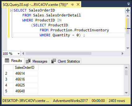
FIGURE 3-2: Orders that contain products that are out of stock.
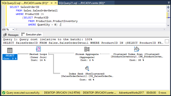
FIGURE 3-3: An execution plan for a query showing orders for out-of-stock products.
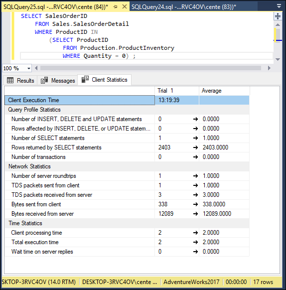
FIGURE 3-4: Client statistics for a query showing orders for out-of-stock products.
This was a pretty efficient query. 12,089 bytes were transferred from the server, but total execution time was only 2 time units. The execution plan shows that a nested loop join was used, taking up 14% of the total time consumed by the query.
How would performance change if the WHERE clause condition was inequality rather than equality?
SELECT SalesOrderID
FROM Sales.SalesOrderDetail
WHERE ProductID IN
(SELECT ProductID
FROM Production.ProductInventory
WHERE Quantity < 10) ;
Suppose you don’t want to wait until a product is out of stock to see if you have a problem. Take a look at Figures 3-5, 3-6, and 3-7 to see how costly a query is that retrieves orders that include products that are almost out of stock.
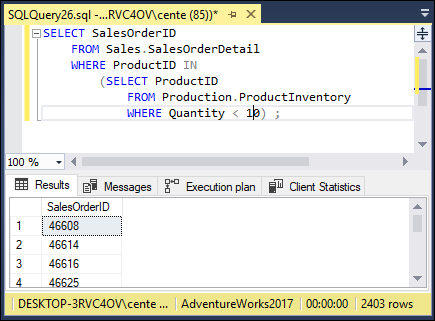
FIGURE 3-5: A nested query showing orders that contain products that are almost out of stock.
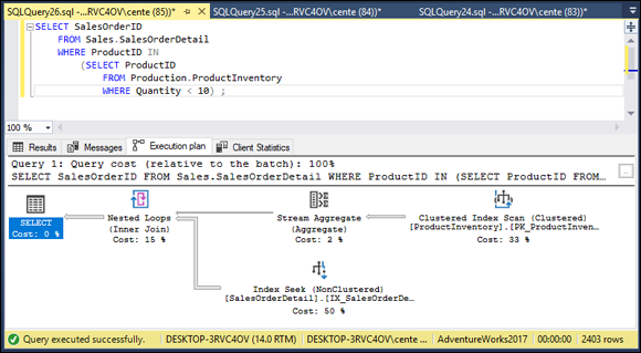
FIGURE 3-6: An execution plan for a nested query showing orders for almost out-of-stock products.
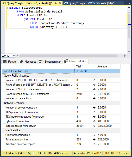
FIGURE 3-7: Client statistics for a nested query showing orders for almost out-of-stock products.
Figure 3-4 shows that 2403 rows were returned, and Figure 3-7 shows that 2404 rows were returned. This must mean that there is one item where there is somewhere between 1 and 9 units still in stock.
The execution plan is the same in both cases. This indicates that the query optimizer figured out which of the two formulations was more efficient and performed the operation the best way, rather than the way it was coded. The client statistics vary. The difference could have been due to other things the system was doing at the same time. To determine whether there is any real difference between the two formulations, they would each have to be run a number of times and an average taken.
Could you achieve the same result more efficiently by recoding with a relational operator? Take a look at an alternative to the query with the inequality condition:
SELECT SalesOrderID
FROM Sales.SalesOrderDetail, Production.ProductInventory
WHERE Production.ProductInventory.ProductID
= Sales.SalesOrderDetail.ProductInventory
AND Quantity < 10) ;
Figures 3-8, 3-9, and 3-10 show the results.

FIGURE 3-8: A relational query showing orders that contain products that are almost out of stock.

FIGURE 3-9: The execution plan for a relational query showing orders for almost out-of-stock products.
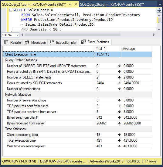
FIGURE 3-10: Client statistics for a relational query showing orders for almost out-of-stock products.
Figure 3-8 shows that the same rows are returned. Figure 3-9 shows that the execution plan is different from what it was for the nested query. The stream aggregate operation is missing, and a little more time is spent in the nested loops. Figure 3-10 shows that total execution time has increased substantially, a good chunk of the increase being in client processing time. In this case, it appears that using a nested query is clearly superior to a relational query. This result is true for this database, running on this hardware, with the mix of other work that the system is performing. Don’t take this as a general truth that nested selects are always more efficient than using relational operators. Your mileage may vary. Run your own tests on your own databases to see what is best in each particular case.
Tuning Correlated Subqueries
Compare a correlated subquery to an equivalent relational query and see if a performance difference shows up:
SELECT SOD1.SalesOrderID
FROM Sales.SalesOrderDetail SOD1
GROUP BY SOD1.SalesOrderID
HAVING MAX (SOD1.UnitPrice) >= ALL
(SELECT 2 * AVG (SOD2.UnitPrice)
FROM Sales.SalesOrderDetail SOD2
WHERE SOD1.SalesOrderID <> SOD2.SalesOrderID) ;
This query into the AdventureWorks2017 database extracts from the SalesOrderDetail table the order numbers of all the rows that contain a product whose unit price is greater than or equal to twice the average unit price of all the other products in the table. Figures 3-11, 3-12, and 3-13 show the result.
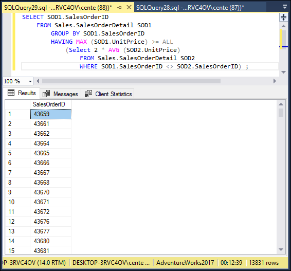
FIGURE 3-11: A correlated subquery showing orders that contain products at least twice as costly as the average product.
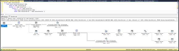
FIGURE 3-12: An execution plan for a correlated subquery showing orders at least twice as costly as the average product.
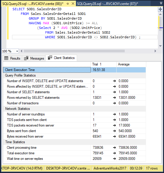
FIGURE 3-13: Client statistics for a correlated subquery showing orders at least twice as costly as the average product.
As shown in the lower right corner of Figure 3-11, 13,831 orders contained a product whose unit price is greater than or equal to twice the average unit price of all the other products in the table.
Figure 3-12 shows the most complex execution plan in this book. Correlated subqueries are intrinsically more complex than are the noncorrelated variety. Many parts of the plan have minimal cost, but the clustered index seek takes up 71% of the total, and the stream aggregate due to the MAX set function takes up 29%. The query took much longer to run than any of the queries discussed so far in this chapter.
The client statistics table in Figure 3-13 shows that 69,341 bytes were returned by the server and that the total execution time was 759,145 time units. As shown in the bottom right corner of the statistics panel, the query took 12 minutes and 39 seconds to execute, whereas all the previous queries in this chapter executed in such a small fraction of a second that the result seemed to appear instantaneously. This is clearly an example of a query that anyone would like to perform more efficiently.
Would a relational query do better? You can formulate one, using a temporary table:
SELECT 2 * AVG(UnitPrice) AS TwiceAvgPrice INTO #TempPrice
FROM Sales.SalesOrderDetail ;
SELECT DISTINCT SalesOrderID
FROM Sales.SalesOrderDetail, #TempPrice
WHERE UnitPrice >= twiceavgprice ;
When you run this two-part query, you get the results shown in Figures 3-14, 3-15, and 3-16.

FIGURE 3-14: Relational query showing orders that contain products at least twice as costly as the average product.

FIGURE 3-15: An execution plan for a relational query showing orders for almost out-of-stock products.

FIGURE 3-16: Client statistics for a relational query showing orders for almost out-of-stock products.
This query returns the same result as the previous one, but the difference in execution time is astounding. This query ran in 8 seconds rather than over 12 minutes.
Figure 3-15 shows the execution plans for the two parts of the relational query. In the first part, a clustered index scan takes up most of the time (93%). In the second part, a clustered index scan and an inner join consume the time.
Figure 3-16 shows a tremendous difference in performance with the correlated subquery in Figure 3-13, which produced exactly the same result. Execution time is reduced to 8 seconds compared to 12 minutes and 39 seconds.
 If you have a similar query that will be run repeatedly, give serious consideration to performing a relational query rather than a correlated subquery if performance is an issue and if an equivalent relational query can be composed. It is worth running a couple of tests.