CHAPTER 10
Fragility Analysis of Goals‐Based Inputs
“You are only entitled to the action, never to its fruits.”
—Bhagavad Gita
“We usually just put in 3% for an inflation estimation. It doesn't really matter too much, anyway,” a trainer responded to my question about the new financial planning software the firm had brought on. It carried numerous assumptions: the returns and volatilities of various assets, the future inflation rate, medical cost increases, even future tax estimations. As a young financial advisor, I understood few of the other inputs, but I could grasp inflation, so that is what I asked about. Despite my trainer's answer, I later played with the inflation assumptions in the tool and found that, contrary to his response, the inflation assumption does matter. It matters quite a lot, in fact. In a few of the simulations I ran, the difference between a 3% inflation rate and a 5% inflation rate over 25 years was the difference between retiring with near certainty and not retiring with near certainty. Counter to my intuition, adjusting the market return assumptions by the same 200 basis points had a much smaller effect. This left me with a question: Which assumptions matter most to goals‐based investors? We know that all our myriad forecasts are wrong to some extent. With limited time and resources, what should we, as practitioners, focus on getting as right as possible, and what can we leave for broader approximations?
I really had no way of effectively answering this question, so I sat on it for years—until I came upon Nassim Taleb's theory of fragility. Most practitioners are familiar with Taleb's iconoclastic style and more laymen‐oriented work, such as The Black Swan. His book Antifragility is a must‐read, but it was his technical work on the topic of system fragility that triggered a possible path to answer this latent question of mine. In 2012, with some coauthors, Taleb published a paper for the International Monetary Fund offering a simple heuristic for detecting fragility in any modellable system.1 These ideas were later expanded into more technical definitions,2 but the heuristic is sufficient for our needs.
In a nutshell, Taleb argues that linear increases in event significance often result in exponential increases in harm to the system. As an example: running a stop sign at 15 miles per hour is a fender‐bender—likely a few thousand dollars in damage. Running a stop sign at 45 miles per hour is a hospital visit—likely tens of thousands of dollars in bodily damage, not to mention the possible loss of life. A 3x increase in event size (speed) resulted in a 10x to 20x increase in harm (financial cost and bodily risk). In derivatives trading, this is known as gamma risk, or convexity.
Taleb uses this starting point to suggest a simple rule. Take a model of the system. Perturb the inputs, one at a time, equally to the upside and downside. Take the average of the output and subtract it from the baseline. If the result is negative, then negative convexity is present and the system is fragile with respect to that input. If the result is positive, then positive convexity is present and the system is antifragile (that is, it gains from extreme movements). If the result is 0, then the system is robust (immune to movements). What is more exciting is that the accuracy of the system model is of secondary importance. As Taleb and Douady put it, “A wrong ruler will not measure the height of a child, but it will certainly tell us if he is growing.” It is not the absolute result with which we are concerned—that is, we are not concerned whether 8 comes out if 4.5 goes in. Rather, we are concerned with the drama associated with the changes—if 8 comes out when 4.5 goes in and 25 comes out when 5 goes in, we have some ground to say that getting this input right is very important.
More formally: Let ![]() be your model of a system and let
be your model of a system and let ![]() be an input to your model (since we are perturbing the model one variable at a time,
be an input to your model (since we are perturbing the model one variable at a time, ![]() represents any input to the model). From here, we perturb
represents any input to the model). From here, we perturb ![]() by
by ![]() , or some constant amount, and subtract the baseline from the average result:
, or some constant amount, and subtract the baseline from the average result:
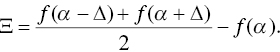
As mentioned above, when ![]() the system is antifragile with respect to
the system is antifragile with respect to ![]() , when
, when ![]() the system is fragile with respect to
the system is fragile with respect to ![]() , and when
, and when ![]() the system is robust with respect to
the system is robust with respect to ![]() . Of course, each input will affect the system differently, so it may be antifragile with respect to one input and fragile with respect to another.
. Of course, each input will affect the system differently, so it may be antifragile with respect to one input and fragile with respect to another.
In the context of financial planning and goals‐based investing, once we understand which variables create the most fragility in our system, we can know where we need to most direct our focus and expertise. The goals‐based utility model carries five basic inputs, and we will test each one: (1) current wealth, (2) future required wealth, (3) time until the funding is needed, (4) expected portfolio return, and (5) portfolio volatility. There are, in fact, some hidden variables in each of these, as well. How much wealth is required to fund a goal is itself a function of our inflation projection, and our current wealth dedicated to a goal is a function of the goal's value relative to the other goals in the investor's goals‐space as well as the number of dollars in an account. If we include the present value of future human capital, current wealth becomes even more nuanced as that calculation carries even more assumptions! Ultimately, the goals‐based model is intricate. Teasing apart each variable is admittedly difficult and quite possibly fraught. Even so, I believe that some light on the question is better than no light.
First, we must build a model that approximates the real world. As mentioned above, this fragility test has quite a lot of tolerance for model inaccuracy (in fact, it assumes the model is inaccurate), which is an immense relief! This allows us to simplify the problem considerably, and can even justify the use of a Gaussian return assumption, which we know is an entirely inaccurate way to model real‐world returns.
Leaning on a Monte Carlo approach, let's model our baseline future value as
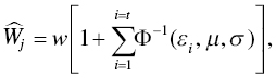
where ![]() is the future wealth value in the
is the future wealth value in the ![]() simulation,
simulation, ![]() is the current wealth value dedicated to the goal,
is the current wealth value dedicated to the goal, ![]() is the time horizon within which the goal must be achieved,
is the time horizon within which the goal must be achieved, ![]() is the inverse cumulative distribution function,
is the inverse cumulative distribution function, ![]() is a uniform random variable that takes values between 0 and 1,
is a uniform random variable that takes values between 0 and 1, ![]() is the location parameter of the distribution (mean), and
is the location parameter of the distribution (mean), and ![]() is the scale parameter (volatility). In essence, this equation simulates the life of a portfolio, starting at the present value and ending at some number of years in the future. Each time subperiod is generated by pulling a randomly selected percentile from the distribution, then applying the aggregate growth factor to the present value of the portfolio.
is the scale parameter (volatility). In essence, this equation simulates the life of a portfolio, starting at the present value and ending at some number of years in the future. Each time subperiod is generated by pulling a randomly selected percentile from the distribution, then applying the aggregate growth factor to the present value of the portfolio.
Using this stochastic simulation approach, we can set ![]() equal to some high number of simulations and thereby assess the probability of meeting our future goal by counting the number of trials that meet or exceed our minimum required future wealth value, then dividing that number by the total number of trials simulated,
equal to some high number of simulations and thereby assess the probability of meeting our future goal by counting the number of trials that meet or exceed our minimum required future wealth value, then dividing that number by the total number of trials simulated, ![]() . More formally:
. More formally:
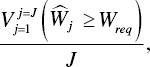
where ![]() is a counting function, returning the number of occurrences where the parenthetical statement is true, or the number of times we hit our goal (simulated wealth is greater than or equal to the minimum required wealth). This equation simply returns the probability of success, which is the litmus test for goals‐based investors. Harm, to goals‐based investors, is failing to achieve their goals.
is a counting function, returning the number of occurrences where the parenthetical statement is true, or the number of times we hit our goal (simulated wealth is greater than or equal to the minimum required wealth). This equation simply returns the probability of success, which is the litmus test for goals‐based investors. Harm, to goals‐based investors, is failing to achieve their goals.
Once we have the baseline probabilities, we can begin adjusting each input in turn and measure the change in goal achievement probability. This should give us a sense for which variables are most important. To get a true apples‐to‐apples comparison, we will adjust each variable by varying percentages rather than some arbitrary number. This will keep some consistency across the various variable types.
The results of our fragility test are displayed in the plot. The vertical axis in Figure 10.1 is the fragility measure (![]() )—recall that negative values indicate the model is fragile with respect to that input. This can also be thought of as a measure of average harm of being wrong. Alternatively,
)—recall that negative values indicate the model is fragile with respect to that input. This can also be thought of as a measure of average harm of being wrong. Alternatively, ![]() can be thought of as a measure of convexity for a particular variable. The more negative the figure, the more being wrong can hurt you. Alternatively, the more positive the figure, the more being wrong can help you. The horizontal axis is the percentage by which we perturbed the variables, which can be alternatively thought of as our level of wrongness.
can be thought of as a measure of convexity for a particular variable. The more negative the figure, the more being wrong can hurt you. Alternatively, the more positive the figure, the more being wrong can help you. The horizontal axis is the percentage by which we perturbed the variables, which can be alternatively thought of as our level of wrongness.
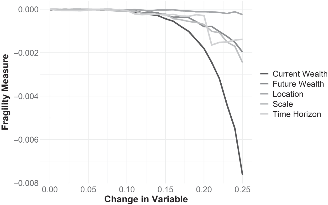
FIGURE 10.1 Fragility Test Results
What becomes immediately clear is how fragile goals‐based investors are with respect to their levels of current wealth. More than any other variable, being wrong about the amount of current wealth available to achieve a goal is, by far, the most damaging. This is unfortunate since current wealth itself involves so many variables. Total account value wealth is often what we think of when we discuss this variable, but it also includes the present value of all future savings. That present value of future savings contains numerous assumptions, such as a growth rate for savings, a discount rate, and we typically do not even consider those events that could cause a serious drop in savings rates (like poor health, divorce, or unexpected children).
The amount of current wealth dedicated to a goal also includes the allocation from the total pool of wealth derived from the optimization engine. This, of course, relies on an accurate gauge of the relative value of one goal to another. Goal valuation, then, is also an input to current wealth. All of these calculations are within the practitioner's purview, and, though practitioners tend to spend most of our time on developing capital market expectations, we might do better to spend more time on getting this variable as right as possible!
In addition, it is not uncommon for people to mentally (or actually) dedicate the same pool of wealth to multiple goals. Withdrawing retirement funds for a vacation home, for example, or using college savings to fund a vacation. As our fragility analysis shows, this can be absolutely catastrophic to a plan. “Double dipping” assets is a sure way to not achieve goals. This, of course, is outside the practitioner's purview. Like most of my fellow practitioners, I have cajoled, begged, and pleaded with clients to not withdraw retirement funds for other purposes. Tax penalties are a good talking point, to be sure, but the real problem is that I know it means my client will severely curtail her ability to achieve her goal by doing so, as this analysis reinforces.
Deciding which variable carries the second most fragility is a bit of a tossup. Time horizon, volatility, and future wealth are all about the same and may trade places across the scale of wrongness. In my original tests,3 I found future values to be the second most fragile, whereas in this one I found volatility to be second most fragile. The other goal variables all matter, of course, and some of the (minor) differences are likely from where one chooses to place the variables in relation to each other in the various tests. In the end, all of these variables are about equally important, but I will take them in the order that this test ranked them.
Second most fragile is our estimation of the scale parameter (volatility). Getting that wrong is not nearly as bad as getting current wealth wrong, but goal achievement is certainly fragile with respect to it. We discussed in a previous chapter how market returns were decidedly non‐normal, and what that means to goals‐based investors. Viewed in that light, that volatility—or the spread of possible outcomes—carries the fragility it does should both come as no surprise and also as a warning to practitioners. If the volatility of possible outcomes is not definite, but rather infinite, as is the case with alpha‐stable distributions, this fragility analysis shows that employing the correct distribution model—or at least employing risk controls informed by the correct distribution model—is extremely important. Indeed, that volatility carries the fragility it does is why investors fear mistimed extreme drawdowns in their portfolio. Investors instinctively know that markets can rob them of their ability to achieve goals just as much as they can grant them the selfsame ability. This is intuitive. What is not necessarily intuitive is how to organize a portfolio of investments or trading rules around such facts—hence the discussion in our earlier chapter.
Of course, portfolio volatility is itself a function of numerous inputs. The volatility of individual investments, their correlations to one another, and how that volatility scales through time, all interact to produce what we see as portfolio volatility. Time on these variables is well spent by practitioners, and, likely, volatility is the least predictable of them all! We can take some comfort in how the exponential nature of the harm only really begins to take hold for higher levels of wrongness (above the 15% level). We don't need to be right to five decimal places. There is a 30%‐point range within which to reasonably forecast: that is, if realized portfolio volatility is 16%, any forecast within the 11% to 21% range will probably do just fine. If, however, we forecast 15% and realized volatility is 30%, our client has a problem. The point is, getting it about right is acceptable. Getting it blatantly wrong is not.
Future wealth is the next most fragile variable. It seems somewhat obvious on the face of it: If we estimate that you need $1 in 20 years, but in fact you need $1.10, we are more likely to have a shortfall. The trouble here is that estimating an exact future value requires triangulating several variables. For longer‐lived and longer‐term goals, like funding a lifestyle, we do not dedicate a lump sum to “buy” that goal one day,4 unlike a piece of real estate or philanthropic gift. Therefore, calculating how much we need to properly fund an ongoing goal is really a function of our capital market expectations over the future period within which the withdrawals are active, and, more importantly, how strongly inflation erodes the purchasing power of our wealth.
Inflation really cannot be understated. Over a period of 20 years, the difference between a 3% inflation rate and a 5% inflation rate is the difference between needing $1.00 and $1.46 when it comes time to fund the goal—a 46% higher wealth requirement. What is worse and more realistic: for goals requiring ongoing distributions where the money is already saved, inflation does even more damage. Assuming markets deliver about the same returns, an investor needs double the amount of money to maintain the same ongoing distributions in a 5% inflation rate scenario versus a 3% inflation rate scenario.5 To maintain buying power in a 3% inflation scenario, we need $25 for every $1 in distributions, and in a 5% inflation scenario we need $50 for every $1 in distributions (assuming a 7% portfolio return for both scenarios).
Clearly, understanding how much wealth we need to support an ongoing spending goal is heavily dependent on inflation. Hence, this is a variable that is worth spending time on. Unlike my original training with the financial planning software, inflation estimates really do matter quite a lot.
Time until a goal is about as fragile as our required future wealth estimates. Fortunately, of all the variables, this is probably the least troublesome. For the most part, this is outside the purview of the practitioner. Clients typically have an idea of how long they can wait until they need the funds. Life happens, of course, but that is difficult to plan for ahead of time. Some goals do maintain their distance from now, like estate goals, for instance. Rarely do people know the year of their death, so an estate goal may always be 7–10 years from now. That is okay, in my view, and, unlike the other variables in the calculation, the practitioner can let this variable be what it is.
Both future wealth and time horizon operate within about the same “wrongness window.” That is, for both variables, being 15% wrong is only slightly more asymmetric to the downside. Once our wrongness moves beyond that level, convexity takes over and downside wrongness begins to dominate.
Finally, and surprisingly, estimates of portfolio return carry the least fragility in the calculation. This is surprising to me since, if the uncountable number of annual capital market expectations that are produced every year is any guide, firms spend an inordinate amount of time pinning down a return estimate for capital markets. Obviously, having some idea of returns is important. We do need an input into the probability function, after all. But, counter to our intuition and our focused efforts, this is a variable where being wrong is not all that harmful. As this analysis shows, firms would do considerably better to spend their time and energy pinning down more accurate inflation forecasts, and still better to spend time understanding their clients and the nature of their client's current wealth. Of course, inflation forecasts do not have the same sizzle as a take on market returns, and, to be fair, clients expect a story around market returns in the coming period. When asked, responding “returns aren't an important variable” is probably a sure way to be fired by a client. When asked whether portfolio return estimates are important, can you imagine if my trainer had responded, “It doesn't really matter too much, anyway”?! Yet that response would have been more accurate with respect to market returns than it was for inflation forecasts!
Time is a valuable resource, especially in the money management business. Dedicating the proper time to the proper questions is what we as practitioners are paid to do. While we do need forecasts for all of these variables, it is better to understand which forecasts require our detailed attention and which can be more roughly estimated. Forecasts are, of course, wrong by some degree no matter how hard we try, but each forecast carries a “wrongness range” within which we need to operate. If we are consistently falling outside of that range, then we are doing our clients a disservice. For most variables, as this analysis reveals, falling within 15% of the realized result is probably sufficient, though getting current wealth more right would be better.
A few grains of salt the reader should take along with this chapter. First, we should remember that fragility analysis is really a measure of convexity; a comparison of how much more damaging being wrong in one direction is relative to the other direction. Obviously, for all of these variables it is better to be wrong in one direction than the other. It would be generally better, for example, to overestimate coming inflation by 15% than to underestimate it by 15%. This builds a cushion into portfolios and, more importantly, aligns with the tried‐and‐true advice “under promise and over deliver.”
I cannot claim, however, that purposefully overestimating variables like inflation in the name of prudence is always a net benefit. Recall that we are required to allocate wealth across goals as well as to investments within them. Purposefully overestimating important variables will send more wealth to priority goals and less wealth to aspirational goals. This means that less important goals will be considerably less likely to be achieved. In short, purposefully misestimating variables yields a misallocation of wealth both across goals and across investments. Of course, investors could theoretically rebalance wealth from one goal to another as inflation actualizes over the years, but that is curtailed by real‐world frictions like varying account types. We cannot realistically pull wealth from an overallocated retirement goal that is executed using a 401(k), or an overallocated college savings goal that has been tied up in a 529 account. Such withdrawals carry prohibitive tax consequences and penalties. In the end, the practitioner must employ experience and wisdom along with quantitative techniques to find the right balance of caution and accuracy in the estimation of critical variables.
Lastly, it is worth noting that my original fragility analysis found a slightly different order for the variables. That analysis was conducted with different baseline assumptions, implying that the fragility of a portfolio may be itself somewhat dependent on our baseline scenario. This is consistent with fragility theory, so it is not particularly noteworthy. Interestingly, in that original analysis, it was misestimation of present value that created the most harm—consistent with the analysis herein. This should again encourage practitioners that a clear understanding of a client situation is absolutely time well spent. After current wealth, my original analysis found that wrongness of future value was second‐most fragile, then time horizon as the third‐most fragile. In that analysis, I did not extend wrongness as far as I did in this one. At lower levels of wrongness, this order still holds in the current analysis. Finally, location then scale round out the model's fragility in the original analysis, which differs from the current results. This is a hint that, again, the baseline assumptions will influence the relative importance of the variables.
I am of the mind that understanding where our models are fragile is a critical piece of our own self‐review and self‐due‐diligence. However, we should remember that it is part of a larger picture, part of an overall understanding of our mental maps that can help guide decision‐making only when viewed in the proper context, and when properly internalized. The internalization is important because that is what feeds practitioner intuition. Intuition based on nothing is a detriment, as behavioral finance has shown us. But intuition founded in well‐thought‐out quantitative techniques is of immense value. That is when it becomes the lens through which an effective practitioner sees everything else. Building our intuition around fragility carries an immense value. More than anything, it provides the practitioner with a “spidy‐sense” when working with and building the myriad models that occupy our daily lives.
Notes
- 1 N. N. Taleb, E. Canetti, T. Kinda, E. Loukoianova, and C. Schmieder, “A New Heuristic Measure of Fragility and Tail Risks: Application to Stress Testing,” IMF Working Paper 12/216, 2012.
- 2 N. N Taleb and R. Douady “Mathematical Definition, Mapping, and Detection of (Anti)Fragility,” Quantitative Finance 13, no. 11 (2013): 1677–1689. DOI:
https://doi.org/10.1080/14697688.2013.800219. - 3 Much of this discussion is drawn from my original paper on the topic: F. J. Parker, “Knowing What to Worry About: A Goals‐Based Application of Fragility Detection Theory,” Journal of Wealth Management 20, no. 1 (2017): 10–16. DOI:
https://doi.org/10.3905/jwm.2017.20.1.010. - 4 Brunel calls these “fuzzy goals.”
- 5 If we expect that our investor leaves the inflation rate in the portfolio to compensate for the lost buying power, then our withdrawal rate is governed by our market returns minus the inflation rate:
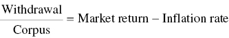 .
.Solving for our required corpus gives:
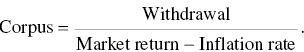
Of course, this does not capture the very important role of volatility in shaping sustainable withdrawals!