
CHAPTER 3
Allocating Wealth Across Goals and Across Investments
“If you want to live a happy life, tie it to a goal.
Not to people or things.”
—Albert Einstein
I admit it seems odd to write a whole book on a theory that can be expressed in a page and a half. Yet, though the presentation of the theory is relatively simple, it is not so simple to put into practice! Most notably, the optimal allocation of wealth to a particular goal depends on the allocation to investments within that goal, and the optimal allocation of investments within a goal also depends on the allocation of wealth to that goal. This recursivity, coupled with the unfamiliar optimization approach, make it worthwhile to spend time solving these problems from the perspective of a practitioner. There are other practical problems, like eliciting the relative goal values from clients. The model takes these points as a given, but they are, in practice, not so straightforward to solicit. This discussion will be about how a practitioner might go about solving these problems, though I will not claim a monopoly on these solutions—others could likely do better! Even so, we shall press ahead, and let us start with the simpler problem first.
How can we ascertain the relative value of goals in an investor's goalsspace? How can we know how much an individual values retirement relative to sending her kids to college, for example, or how much she values funding an estate goal versus buying a vacation home? In the previous chapter, I suggested asking a series of questions: Would you rather send your kids to college with certainty, or retire with a probability of p? We vary p until our investor is ambivalent to the choice. We might think of this as the goals‐based analog of a risk‐tolerance questionnaire. An annoying part of the process, to be sure, but a necessary one.
That said, I feel I must acknowledge my doubts about whether clients have the patience to give feedback at any serious level of granularity. It would be considerably more convenient to have a reasonable approximation of these figures. Practitioners could assume that all “need” goals have a value of 1.00, and perhaps “want” goals have a valuation of 0.75. Or, at the very least, practitioners could use that baseline as a starting point to begin the conversation, calibrating more accurate valuations based on feedback from the client. I genuinely hope the literature on this topic will evolve because I do not feel that my method is particularly client friendly. Though, since I have no better solution, we will have to table the practical problems involved with eliciting goal values, and let us turn to the bigger problem of model recursivity.
The model is recursive because we have to find both the optimal across‐goal allocation (how much wealth we dedicate to each goal) and we have to find the optimal mix of investments within each goal. Both of those allocation levels are in play simultaneously, creating a decided nonlinear problem.1 I find it easiest to work from the bottom up. First, we find the optimal investment allocation within each goal for each potential level of across‐goal wealth allocation. That is to say, we find and log the optimal investment mix when we allocate 1%, 2%, 3%, …, 97%, 98%, 99%, of our total wealth to the goal.
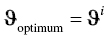
Granularity is an obvious question at this stage—more granularity is better, but we can quickly run into unreasonable computation times and memory needs. If ![]() is our level of resolution (
is our level of resolution (![]() for 1% intervals,
for 1% intervals, ![]() for 5% intervals,
for 5% intervals, ![]() for 10% intervals, etc.) and
for 10% intervals, etc.) and ![]() is the number of goals, then we must calculate and hold in memory
is the number of goals, then we must calculate and hold in memory ![]() portfolios. Five goals run with a resolution of 100 yields
portfolios. Five goals run with a resolution of 100 yields ![]() portfolio calculations that must be made and held in memory. In the end, the practitioner has to make this decision based on the application at hand and the computational resources available. It may well be that a resolution of 20 or 10 is sufficient for a particular application. I do not believe there is one right answer here.
portfolio calculations that must be made and held in memory. In the end, the practitioner has to make this decision based on the application at hand and the computational resources available. It may well be that a resolution of 20 or 10 is sufficient for a particular application. I do not believe there is one right answer here.
Once we have generated optimal portfolios for each goal given each potential level of wealth, we use the results of these optimal investment allocations to inform the optimal across‐goal allocation. Because of the discrete nature of our portfolio allocation results, I recommend using a Monte Carlo engine to simulate various across‐goal allocations and their effects on total utility. Obviously, we are trying to find the across‐goal allocation that yields the highest utility. For each simulation of across‐goal allocation, we match the optimal portfolio for that level of across‐goal allocation and return a probability of achievement. That probability is the input used in the utility function.
Finally, we match the optimal across‐goal allocation with the optimal within‐goal portfolio weights and return the optimal aggregate portfolio (or keep them separate, whichever the implementation strategy demands).
That is the procedure summary. Now, let's tackle the first‐stage optimization algorithm.
Define:
- investment universe of
 ‐number of potential investments.
 - necessary level of resolution, log this as
 .2
.2  ‐number of empty
  matrices, log these as
  .3
.3 returns the parameters of our chosen cdf, given portfolio weights,
  .4
.4 is the lower‐tail cdf with our required return and parameters
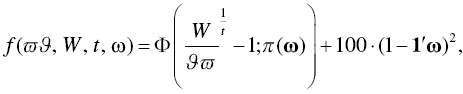
- the objective function as
For ![]() to
to ![]() :
:
- For
 to
to  :
:

- Find
 that satisfies:
- Log
- Find
And we are left with a matrix of optimal investment allocations, ![]() , with each row of the matrix corresponding to a potential across‐goal allocation and each column representing a different investment in our investment universe. Notice how our target function—the function we are minimizing—includes the constraints that the investment weights must sum to 1, and that the investment weights cannot be greater than 1 nor less than 0. The latter is the no‐short‐sell/no‐leverage constraint. These constraints could, of course, be removed or modified by adjusting or eliminating the constraint applied to the investment weights in the optimization function, but I prefer to include them as I know of very few goals‐based investors who would accept leverage and short sales as a matter of core policy.
, with each row of the matrix corresponding to a potential across‐goal allocation and each column representing a different investment in our investment universe. Notice how our target function—the function we are minimizing—includes the constraints that the investment weights must sum to 1, and that the investment weights cannot be greater than 1 nor less than 0. The latter is the no‐short‐sell/no‐leverage constraint. These constraints could, of course, be removed or modified by adjusting or eliminating the constraint applied to the investment weights in the optimization function, but I prefer to include them as I know of very few goals‐based investors who would accept leverage and short sales as a matter of core policy.
This algorithm is pretty straightforward in practice. We are trying to build a matrix where the rows correspond directly to each possible across‐goal allocation and each column corresponds to the weight of an investment in our investment universe. If we have 99 potential across‐goal allocations and, say, 10 potential investments to choose from, then ![]() , our matrix, would have 99 rows and 10 columns. From there, we simply iterate through each potential level of across‐goal allocation and record the investment weights that give us the least chance of failure, given the goal specifics. Of course, we do this for each goal, and each goal will have its own matrix of results.
, our matrix, would have 99 rows and 10 columns. From there, we simply iterate through each potential level of across‐goal allocation and record the investment weights that give us the least chance of failure, given the goal specifics. Of course, we do this for each goal, and each goal will have its own matrix of results.
Our second stage of optimization is to combine the across‐goal allocations in such a way as to deliver the highest utility. Obviously, our previous optimization was not continuous—that is, we had to choose some level of resolution and optimize over each of those specific values. So, our second stage algorithm cannot be continuous, either. Given discrete optimization, there is no guarantee that we have found the solution that is exactly correct. I lose no sleep over this. The practitioner will need to find the level of resolution that best balances computing time and estimation accuracy for the project at hand, but there is no sense in “being wrong to several decimal points,” as Jean Brunel has cautioned.
One more note before moving forward. Whereas more traditional nonlinear optimizers can be deployed on the target function in the first optimization algorithm, I employ a Monte Carlo technique in the second stage. I find it is simple, effective, and takes minimal computing time. Again, I will leave it to the practitioner to find the right balance for her own application. Keeping the notation from our first algorithm going, the second stage of optimization is as follows.
Define:
- the number of simulation trials as

 as the vector of
  ‐number of simulated across‐goal allocations, subject to


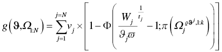
- the objective function5 is
For ![]() to
to ![]() :
:
- if
- then
- else next
Return:
In summary, we are simulating many possible allocations of wealth to each goal until we find the mix that delivers the maximal balance of achievement probabilities and goal values. We simulate some number of potential across‐goal allocations, One simulated value at a time is plugged in for ![]() in the optimization function above. From the goal's matrix (
in the optimization function above. From the goal's matrix (![]() ) we pull the row of investment weights that matches the across‐goal allocation we are testing, written as
) we pull the row of investment weights that matches the across‐goal allocation we are testing, written as ![]() (the matrix for goal
(the matrix for goal ![]() , row number defined as
, row number defined as ![]() , and columns
, and columns ![]() through
through ![]() ) and we log the mix of those across‐goal allocations that delivers the maximal utility across all simulations. Finally, we return the optimal across‐goal wealth allocation and the optimal investment weights for each goal. When implementing, then, we can either keep the accounts separate or aggregate the optimal weights into a single portfolio, whichever is preferred.
) and we log the mix of those across‐goal allocations that delivers the maximal utility across all simulations. Finally, we return the optimal across‐goal wealth allocation and the optimal investment weights for each goal. When implementing, then, we can either keep the accounts separate or aggregate the optimal weights into a single portfolio, whichever is preferred.
CASE STUDY
Let's consider a case study together to help illustrate the procedure. For interested readers, I have included the relevant R code script as part of the book supplement. Again, I want to stress that the actual procedure may not be optimal from a computational perspective—I would encourage other practitioners and researchers to develop their own approach—but it suffices for my purposes.
A client joins our firm. Our first step as advisors is to spend ample time in conversation. We need to fully understand her goals, her tax situation, her ethical constraints (more on that later), and so on. We must also ensure that she has reasonable expectations, both of herself and us. We should never take on a client with unreasonable expectations or a client mandate that is not within our ability. This conversation is, then, a two‐way street, determining whether this client will fit within our process as well as for the client to get a handle on her financial goals and financial picture.
Another objective at this stage is to help the client dream a little. I have found that, very often, clients do not have a clear picture of their goals. One of an advisor's jobs is to help the client crystalize her objectives. They are changeable, of course, and communicating that point is important, as well; clients will have a harder time committing to 30‐year objectives that they feel can never be updated. This involves plenty of listening as clients talk themselves through their needs, wants, wishes, and dreams. We need to spend time forecasting our client's psychological state (“how would you feel if…”), as well as forecasting their financial state (“what is your pattern of raises…”). Client homework is not uncommon after the first meeting or two.
After ample conversation, we determine that our new client has the following goals in her goals‐space:
- She wants to leave an estate to her children of $5,000,000, planned in 30 years from now.
- She needs to maintain her lifestyle expenses starting in 10 years, and we estimate that she will need $5,157,000 to do that.
- Our client would like to purchase a vacation home in 4 years, and her estimated price is $713,500.
- If possible, our client would like to donate $8,812,000 to her alma mater sometime around 18 years from now. This donation carries naming rights to a building on campus.
- Currently, our client has $4,654,400 in wealth from which to draw to fund her goals.
And with her goals fleshed out, we must now determine their value relative to one another. First, we have our client rank‐order her goals from most important to least important. Here are the results of her goal ranking:
- Living expenses
- Children's estate
- Vacation home
- Naming rights
We now ask our client a series of questions and log the results:
- Would you rather achieve your children's estate goal with certainty or your living expenses goal with probability p?
- Would you rather buy your vacation home with certainty or achieve your children's estate goal with probability p?
- Would you rather fund your alma‐mater with certainty or buy your vacation home with probability p?
At each stage, we vary p until she is indifferent to the choice. In our case study, our client has responded, and we have logged the value ratios as:
- 1.00 for her living expenses goal
- 0.45 for her estate goal
- 0.50 for her vacation home goal
- 0.58 for her naming rights goal
Recall, there are two steps to determining a goal's value. The first is the value ratio of each goal—the raw results we just elicited from our client. To determine the actual value of each goal, however, we have to take the cumulative product of the value ratios, from the most important up to the goal we are considering. So, our living expenses goal gets an automatically assigned value of 1.00. Our client's estate goal gets a value of ![]() , which is the value of the living expenses goal times the value ratio of her estate goal. The vacation home goal gets a value of
, which is the value of the living expenses goal times the value ratio of her estate goal. The vacation home goal gets a value of ![]() , which is the product of the value ratios for the living expenses goal (1.00), the estate goal (0.45), and the vacation home goal (0.50). Her naming rights goal gets a value of
, which is the product of the value ratios for the living expenses goal (1.00), the estate goal (0.45), and the vacation home goal (0.50). Her naming rights goal gets a value of ![]() . Hence, the rank‐ordered goals have declining values, as we would expect:
. Hence, the rank‐ordered goals have declining values, as we would expect: ![]() .6
.6
With the details of her goals fleshed out, we can couple our client's goal details with our firm's capital market expectations and run our optimization procedure. Obviously, capital market expectations are a critical step. Better forecasts yield better outcomes. It is not my intent to write a book about building a better investment philosophy—there are plenty of those in the world written by practitioners with much more skill than I have! It is here, however, that investment teams infuse their own belief about markets, and that can add considerable value when done well. For the sake of our illustration, let us suppose our capital market expectations are those listed in Table 3.1.
TABLE 3.1 Sample Capital Market Expectations
| E (return) | E (volatility) | |
|---|---|---|
| Equity | ||
| Large Cap | 0.09 | 0.15 |
| Mid Cap | 0.11 | 0.16 |
| Small Cap | 0.12 | 0.17 |
| Int'l Developed | 0.07 | 0.15 |
| Emerging Markets | 0.09 | 0.17 |
| Fixed Income | ||
| US Agg Bond | 0.04 | 0.05 |
| US High Yield | 0.06 | 0.09 |
| US Treasury | 0.03 | 0.03 |
| Corporate | 0.05 | 0.07 |
| Alternatives | ||
| Gold | 0.06 | 0.19 |
| Oil | 0.04 | 0.32 |
| Lottery‐Like | ||
| Private Equity | 0.15 | 0.28 |
| Venture Capital | 0.16 | 0.30 |
| Angel Venture | ‐0.01 | 0.82 |
| Cash | 0.01 | 0.001 |
Here is where we employ the optimization algorithm from above. As mentioned, we first find every optimal portfolio for possible allocations of wealth to each goal (![]() , in our equations), subject to some level of resolution,
, in our equations), subject to some level of resolution,![]() . In the plot, I have demonstrated the optimal investment weights (
. In the plot, I have demonstrated the optimal investment weights (![]() , in our equations) for each possible allocation of wealth to our client's living expenses goal, and this was done at a resolution of 100. Meaning, an optimal portfolio was built for a 1% goal allocation, 2% goal allocation, 3% goal allocation, all the way up to a 100% goal allocation, moving in increments of 1% point. Figure 3.1, then, is a visual representation of a goal's allocation matrix,
, in our equations) for each possible allocation of wealth to our client's living expenses goal, and this was done at a resolution of 100. Meaning, an optimal portfolio was built for a 1% goal allocation, 2% goal allocation, 3% goal allocation, all the way up to a 100% goal allocation, moving in increments of 1% point. Figure 3.1, then, is a visual representation of a goal's allocation matrix, ![]() .
.
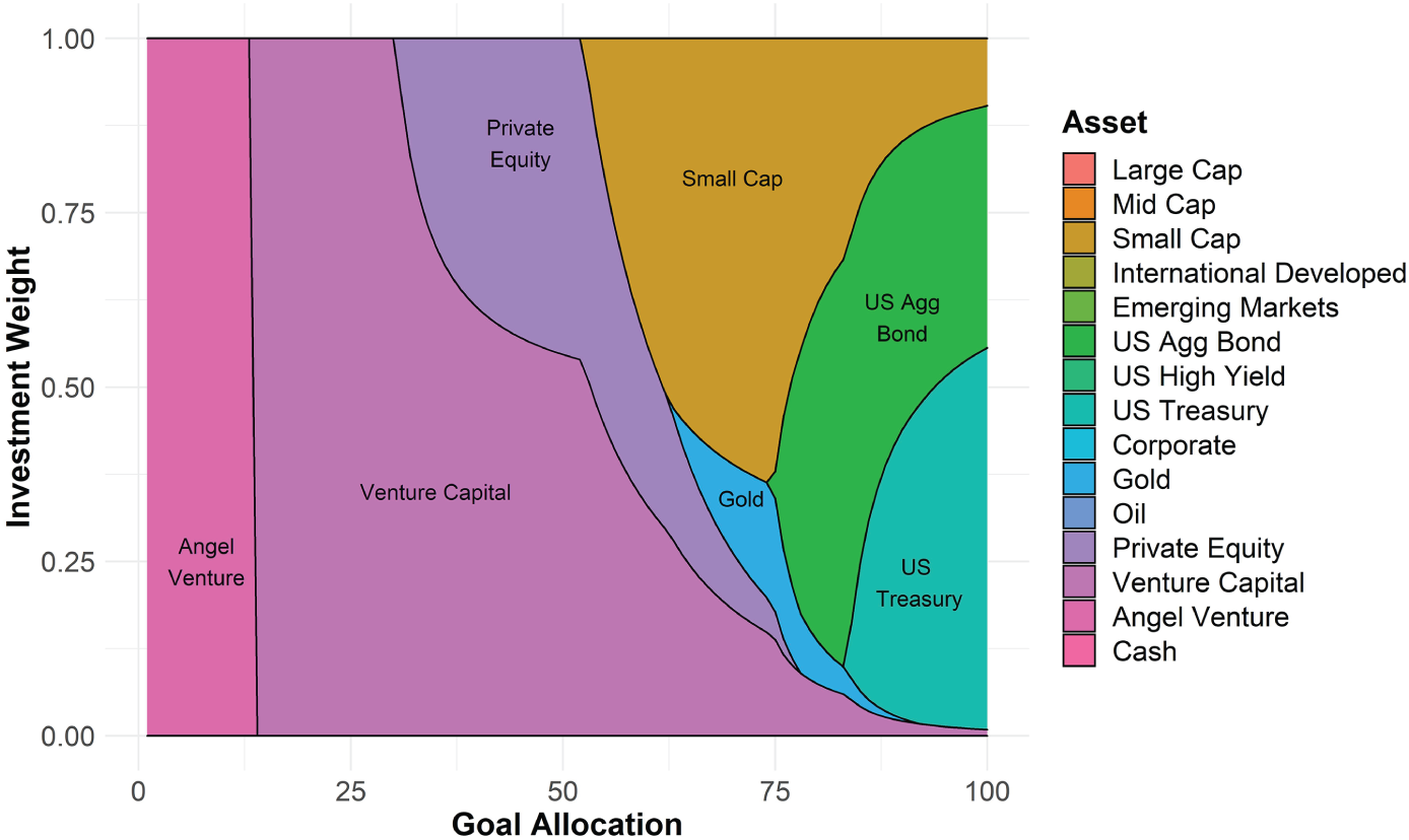
FIGURE 3.1 Optimal Portfolios for Various Levels of Wealth Allocation
Note that there is no 0% goal allocation. The theoretical model insists that some level of resources be dedicated to a goal, no matter how small. If there are no resources dedicated to the goal, then we cannot properly call it a goal. There is a philosophical discussion to be had here, no doubt, but I will spare us all. Suffice it to say, if there are objectives you want to achieve in life, you have to do something in the real world, no matter how small, to move toward their accomplishment. Otherwise they are not goals at all—and that is a mathematical fact.
From here, we go about optimizing the across‐goal allocation of wealth. I use a Monte Carlo simulation at this stage because, as mentioned above, I find it easiest to marry the discrete nature of each within‐goal portfolio with possible across‐goal allocations. In that case, we simulate some large number of potential across‐goal allocations, each of them rounded to match our chosen level of resolution—we will not be able to match a simulated 41.255% goal allocation if our level of resolution is in increments of 10%, so we would have to round 41.255% to 40% before proceeding. For each of those simulations, we pull the probability of achieving each goal with their respective levels of across‐goal allocations, then plug the results in to our utility model. Obviously, we are trying to find the across‐goal allocation mix that yields the highest utility.
Table 3.2 shows the results of the allocation procedure. Our highest valued goal, the living expenses goal, receives 81% of the wealth pool, giving our client a 72% chance of success for that goal. Somewhat surprisingly, the children's estate goal receives only 3% of the wealth pool. Yet, because of the time horizon, the size of the wealth pool, and our capital market expectations, our client has a 55% probability of attaining that goal.7 The vacation home goal receives 15% of the wealth pool, meaning it can be funded today. Note that the allocation engine returns an all‐cash allocation for a fully funded goal; this is a hard‐coded preference of mine but need not always be the case (in many cases, it would not be appropriate). Our aspirational naming‐rights goal garners a 2% allocation of the wealth pool. Because it is valued so low compared to the other goals, and because its achievement is very improbable, anyway, the goal is reliant on the lottery‐like angel venture investment. Even still, it carries a 36% probability of achievement.8
These results quite clearly illustrate the benefits of the goals‐based framework. To begin with, the academic literature has offered no mechanism for allocating wealth across goals. Up to now, the assumption has been that investors have already allocated wealth across their goals, which is an odd assumption, especially considering that so much of the literature assumes investors are not rational. Assuming that investors have already rationally allocated wealth across goals seems silly, at least to me.
What's more, these results can be somewhat counter to our initial intuition. We are fully funding the vacation home, for example, but there is only a 72% chance of maintaining lifestyle expenses. If we directed all resources to this lifestyle funding objective, our client would have an 87% proba‐bility of achieving it. But, for 14% points of achievement probability, our client can buy a vacation home today and fund, with reasonable confidence, her other goals. Again, the goals‐based framework is a tool to rationally trade the achievement of one goal for another, a tool that has been largely absent in the literature to date.
TABLE 3.2 Resultant Optimal Allocation of Wealth, Within and Across Goals
| Not all percentages add to 1 due to rounding. | |||||
|---|---|---|---|---|---|
| Aggregate Portfolio | Living Expenses | Children's Estate | Vacation Home | Naming Rights | |
| Goal Allocation | 81% | 3% | 15% | 2% | |
| Equity | |||||
| Large Cap | – | – | – | – | – |
| Mid Cap | – | – | – | – | – |
| Small Cap | 29% | 36% | – | – | – |
| Int'l Developed | – | – | – | – | – |
| Emerging Markets | – | – | – | – | – |
| Fixed Income | |||||
| US Agg Bond | 42% | 52% | – | – | – |
| US High Yield | – | – | – | – | – |
| US Treasury | – | – | – | – | – |
| Corporate | – | – | – | – | – |
| Alternatives | |||||
| Gold | 4% | 5% | – | – | – |
| Oil | – | – | – | – | – |
| Lottery‐Like | |||||
| Private Equity | 1% | – | 25% | – | – |
| Venture Capital | 7% | 7% | 75% | – | – |
| Angel Venture | 2% | – | – | – | 100% |
| Cash | 15% | – | – | 100% | – |
Modern portfolio theory would also entirely eliminate lottery‐like investments from consideration, and, therefore, our naming‐rights goal would be considered an infeasible goal—it would return an error, in other words, and we would have to change something about the goal's variables or our expectations. We could adapt the goals‐based method to always be consistent with MPT. To do this, we simply maintain exposure to the last portfolio on the efficient frontier, even if the return required by the goal is greater than the return offered by that last portfolio. Doing so would allow us to allocate across our goals, and it would keep all portfolios on the efficient frontier, but it comes at the cost of lower probability of achievement for aspirational goals. For practitioners who are mean‐variance constrained, or for those of us who are reluctant to allocate to lottery‐like investments in a professional setting (it is a brand‐new idea, after all), adapted MPT carries some appeal. I have included the procedure for adapting MPT in the code scripts attached to this chapter.
At any rate, this is a method for solving some of the challenges of allocating wealth in the goals‐based framework. It is, unfortunately, more complicated than the traditional method, carrying an inherent recursivity. Fortunately, that extra complication is easily handled by modern computing power. For investors who choose to remain mean‐variance constrained, the goals‐based framework can be adapted to keep all portfolios on the efficient frontier. The practitioner need only add an instruction in the algorithm to check if the goal's required return is greater than the return offered by the last portfolio on the frontier. If yes, then maintain exposure to the endpoint portfolio.
With our two‐layer allocation problem now solved, I turn to another complex problem which the goals‐based framework allows us to solve: allocating wealth when a portfolio manager has a market view that spans more than one period.
Notes
- 1 Modern portfolio theory has well‐known closed form solutions for finding the optimal investment mix of a portfolio. The goals‐based problem is considerably more complex since it has two layers of optimization occurring simultaneously. If there is a closed‐form solution, it is well beyond my mathematical ability to derive it.
- 2
 is the number of optimal portfolios to calculate, and since possible allocations run from 0 to 1, we know that our intervals,
  , are defined as
  . So,
. So,  yields optimal portfolios for every 20% of allocation to the goal.
  yields optimal portfolios for every 1% of allocation to the goal, and so on.
 - 3 There will be a different matrix for each goal: each row in the matrix represents a potential across‐goal allocation of wealth (rows represent values of
 ), and each column will represent the weight of an investment (columns represent
  ).
). - 4 For example, mean and variance for a Gaussian distribution, location and scale for a logistic distribution, alpha, beta, gamma, sigma for an alpha‐stable distribution, and so on.
- 5 There is a lot going on in this objective function. Effectively, we are just applying the goals‐based utility function: taking the sumproduct of the value of a goal
 and its probability of achievement. Our parameter function is now taking a row‐vector from our
  matrix (columns 1 through
  ), since the matrix holds optimal investment weights for various across‐goal allocations. We can find the needed row number of the matrix by multiplying our chosen resolution,
  , by the simulated across‐goal weight,
  .
. - 6 We could run a quick check of preference consistency here and ask another question: would you rather achieve your naming rights goal with certainty or your living expenses goal with probability p? Clearly, we expect the p to equal something close to 0.131. If it does not, then our client's preferences are not transitive (which is one of our axiomatic assumptions), and we have a problem. It would be worth a research study to measure the consistency of these types of preferences.
- 7 This does not include the value of the vacation home, which would be ultimately included in our client's estate goal.
- 8 This is a cartoon example of course, as the angel venture investment was assumed to have a Gaussian distribution, which it certainly would not. I address non‐Gaussian distributions in a later chapter, but it is worth noting that the practitioner can (and should) model investments like this with a more appropriate distribution.