CHAPTER 5
Real Markets, Real Risk, Real Portfolios
“Foresight is not about predicting the future, it's about minimizing surprise.”
—Karl Schroeder
For the latter‐half of my childhood, I grew up on a working cattle ranch in central Texas. As you can imagine, there is always something to be done on a working ranch—haul hay, feed cattle, work cattle, fix fence, and so on—and this kind of work in the heat of the Texas sun imparts an appreciation for the tools of the trade. No two tools loom larger on working land than the tractor and the horse.
Tractors are quite handy, of course. You can haul hay, fix fence, and plow fields with tractors. The best thing about a tractor, however, is its reliability. So long as it is well‐oiled and full of diesel, you can turn on that tractor and go to work. It does exactly what you tell it to do.
Horses have their own advantages. They are great at reaching those rugged nooks and crannies of land, and almost nothing is better for herding other animals than a good horse. Horses, however, are bigger and stronger than we are, and, unlike tractors, they have a mind of their own. If you wake up to a horse who does not want to work, there really is nothing you can do about it. And, occasionally, a horse gets spooked and decides to buck you off.
In modern finance, replete with our deterministic equations and empirical studies, we have come to view markets as though they were tractors. In our minds, markets have become a tool that we can reliably use to get our work done—to retire, to send kids to college, to fund our philanthropic gifts. But contrary to our imagination, markets are really much more like horses than they are tractors. Wonderful tools, yes, but markets are bigger and stronger than we are, and very often they would just as soon kick us in the teeth as help us get our work done. Goals‐based investing is as much about discarding these incorrect views of markets as it is about adjusting the math of portfolio theory.
As we have explored, there are some silly assumptions pervading the investment literature—unlimited short‐selling and leverage are certainly at the top of that list. There is, however, another very damaging assumption for goals‐based investors pervading the practical and academic literature: the assumption of Gaussian returns for assets. Of course, many academics and practitioners will be quick to point out that though markets may not be exactly statistically normal, they are “close enough” for our purposes. If returns are close enough to Gaussian most of the time, then we could defend the use of such a distribution, I will agree. But is that claim actually true?
Our first clue comes from the S&P 500 index (though any asset would do to illustrate this point). Suppose we were to use the first 1,000 days of returns to calculate an expected volatility, as measured by standard deviation. If returns were drawn from a Gaussian distribution, that would be more than enough to get an accurate expectation. However, what we find is that, no matter how long of a period we use to calculate volatility, any expectation derived from the past is always very wrong going forward.
This difference is illustrated in the plot. Here I have repeatedly calculated the standard deviation of returns over the number of days shown on the x‐axis, and plotted the result on the y‐axis. So, we calculate the standard deviation of daily returns for 100 days, then 101 days, then 102 days, and so on. When drawn from a Gaussian distribution, volatility converges fairly quickly on our expectation, as the dotted line shows. That is, when drawn from a Gaussian distribution, the standard deviation of daily returns is not meaningfully different, whether we use 2,500 days of data or 5,000 days of data, and our standard deviation expectation tends to hold for the next 2,500 or 5,000 days of data. This is what we would expect if markets were tractors.
Actual market returns, however, show that volatility seems to never converge toward any given number, as Figure 5.1 demonstrates. In fact, the longer the period of data, the higher volatility seems to get. Note, too, how the data becomes dominated by intermittent “catastrophes.” Volatility tends to find a stable point, but then it jumps considerably. Even after 12,000 days of data, calculated volatility has not found an equilibrium and continues to drift higher. Sounds quite a lot like a horse. Most of the time we can get our work done, but every now and then that horse tries to buck us off.
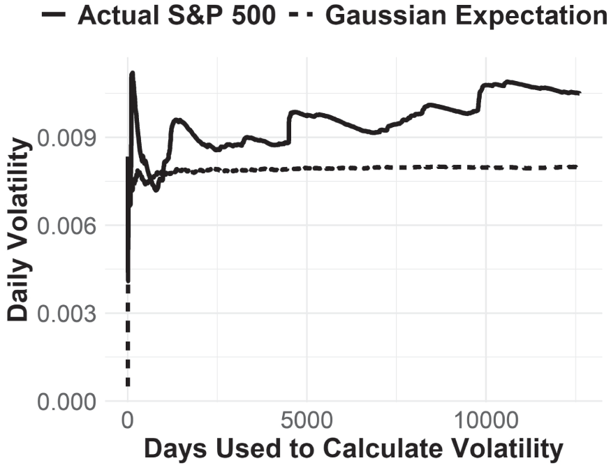
FIGURE 5.1 N‐Day Volatility of S&P 500, Jan 1970 to Dec 2020
If that is not convincing enough, let's absorb the same data a different, more formal, way. Nassim Taleb calls this Wittgenstein's Ruler.1 Suppose you believe, with 99.9% certainty, that market returns are Gaussian. We can use Bayes' rule to update our beliefs rationally in the face of new evidence. We find that there has been one 10‐standard‐deviation move in the S&P 500 across the period 1950 to 2012, and two 9‐standard‐deviation moves.2 So, presupposing markets are Gaussian with 99.9% certainty (our prior), given these market moves (the new evidence), we must accept that the probability of markets actually being Gaussian is 0.0000000000000002%.
In short, there is really no way a rational person can believe market returns are drawn from a Gaussian distribution, or anything close thereto.
Better fitting the evidence of observed returns is a type of distribution known as Levy‐alpha‐stable, sometimes called just alpha‐stable or Levy distributions (Figure 5.2). Among other things, these distributions are characterized by having infinite volatility—there is no point where we can expect calculated standard deviation to settle on a particular value. Our expected volatility, therefore, is infinite with these distributions. Of course, this puts the entirety of mean‐variance theory in doubt—if our variance expectation is always infinite, there is no way to find a portfolio with minimum variance. Luckily for goals‐based investors, alpha‐stable distributions have defined cumulative distribution functions! Since that is the central metric with which we are concerned, goals‐based portfolio theory allows investors to step away from the Gaussian assumption, at least at the portfolio level.
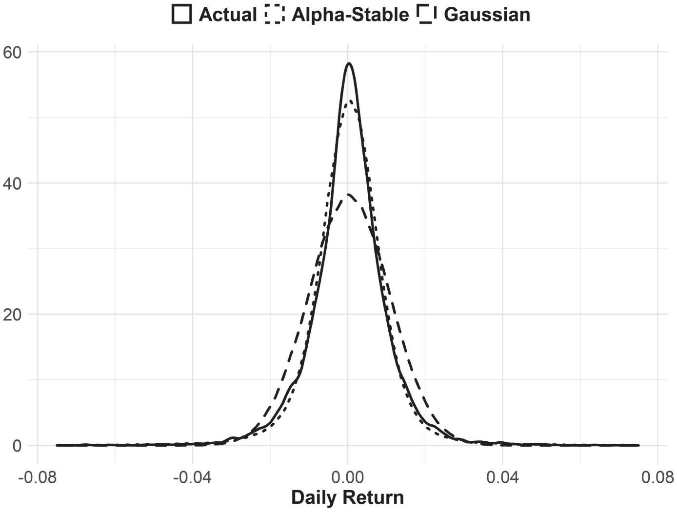
FIGURE 5.2 Daily S&P 500 Returns Compared to Alpha‐Stable and Gaussian Distributions
Another defining characteristic of these distributions is that they have “fat tails.” Returns will be very very bad and very very good much more often than the Gaussian distribution would predict. In the illustration of daily S&P 500 returns, note how in the tail of the actual distribution the record of daily returns very closely matches the alpha‐stable distribution (Figure 5.3).
For goals‐based investors, understanding which return distribution we can expect is extremely important as it yields different outcomes for risk expectations, portfolio allocation and, ultimately, the probability of achieving a goal. For example, suppose you had perfect foreknowledge of the mean and standard deviation of annual returns for a portfolio that was 60% allocated to SPY, 30% to AGG, and 10% to GLD from 2004 through 2020. Even with perfect knowledge of those parameters, using a Gaussian return assumption would lead you to underestimate the probability of achieving a 7% annual return by 13% points (Gaussian assumptions lead to a 57% probability of achieving 7% or better in any given year). Using the alpha‐stable distribution (and assuming perfect foreknowledge of the parameters), we get a probability of 67%—a miss of only 2% points as the actual realized probability is 69%. Gaussian assumptions also underestimate the chances of a severe loss in any given year—an important consideration for investors nearing their goal. As veteran practitioners are well aware, the order of returns matters quite a lot for investments that carry defined time horizons. All of this is illustrated in Figure 5.4.
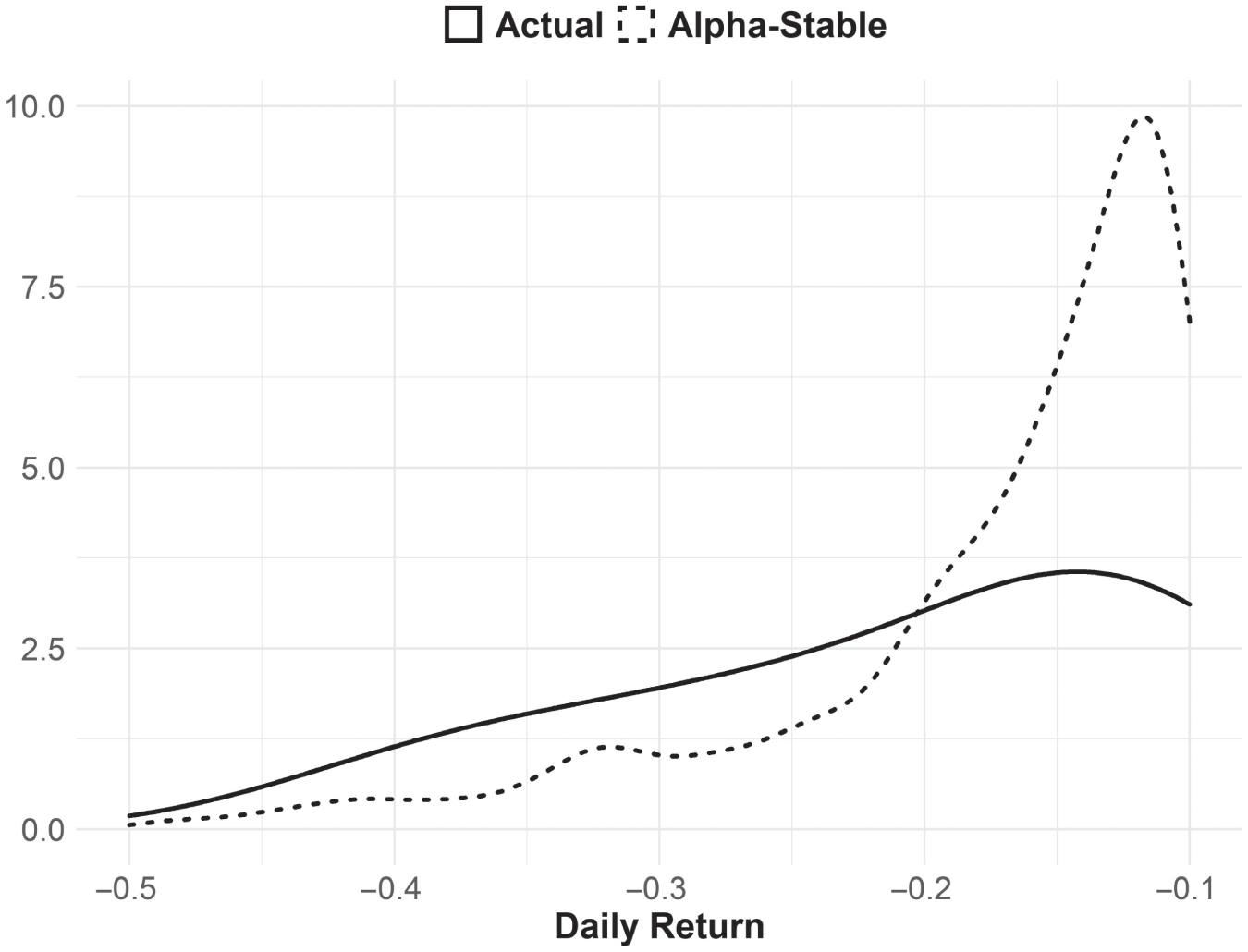
FIGURE 5.3 Daily S&P 500 Returns in the Left Tail Compared to Alpha‐Stable and Gaussian Distributions
As a quick aside, my favorite example of the risk in the order of returns is the comparison of two 30‐year market periods: 1981–2010 versus 1930–1959. Both market periods returned an average of 12.2% per year, but in the second period our investor experienced staggering losses in the first few years (–25% in 1930, –43% in 1931, and –8% in 1932). Of course, for investors not taking withdrawals, this is not much of a problem. These market drawdowns are, in fact, beneficial for investors who are actively contributing to an account because they are buying at lower prices early on. However, for investors who are taking withdrawals, those early losses are catastrophic. An investor withdrawing 6% of her initial portfolio value per year from her account would see it depleted within the first decade. A 6% withdrawal rate sounds excessive, yes, until you compare it to the 1981–2010 period. That period saw very good first years (–5% in 1981, 21% in 1982, and 23% in 1983). During that period, our investor not only withdrew 6% of her initial portfolio value every year but also saw her corpus grow by a factor of 10! For goals‐based investors, the order of returns and the timing of drawdowns matters!
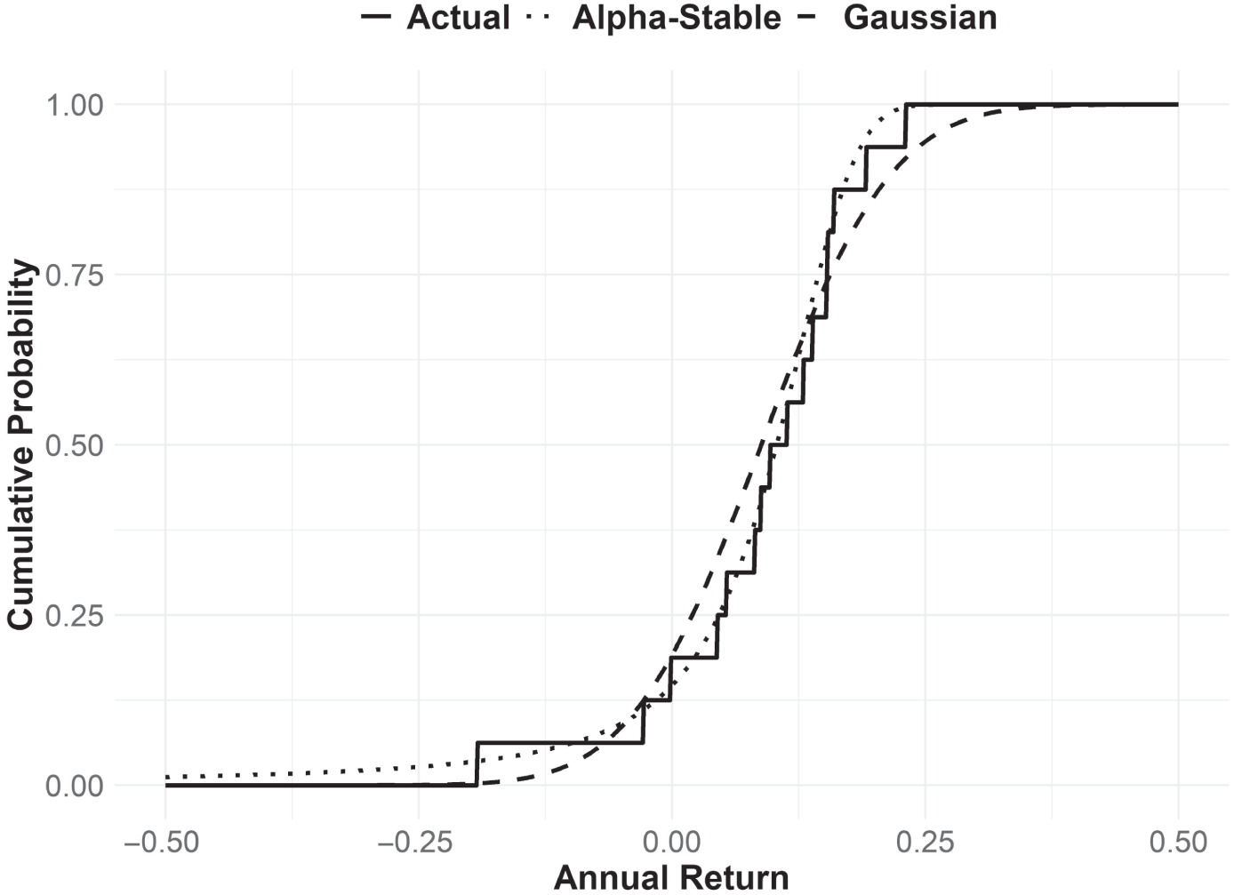
FIGURE 5.4 Cumulative Distribution Function of Actual, Alpha‐Stable, and Gaussian Annual Return Distributions
60% SPY, 30% AGG, 10% GLD Portfolio, 2004–2020
But even that is not our most serious concern. Of most concern is that the Gaussian return assumption allows us to take a shortcut when organizing goals‐based portfolios. When we make the assumption that returns are Gaussian, it is mathematically equivalent to subdivide our total return requirement into annual subperiods, then organize the portfolio to maximize the probability of achieving that return in a single period. In other words, it is the same to optimize the portfolio to achieve a 7% return in the coming year as it is to achieve a ![]() return over a 15‐year period. We are allowed to do this because mean and variance scale quite nicely in a Gaussian distribution: a single‐year mean can be scaled to a five‐year mean by simply multiplying the figure by five. A single‐year standard deviation can be scaled to a five‐year standard deviation by multiplying the figure by the square‐root of five. This shortcut is very handy, but, unfortunately, quite flawed.
return over a 15‐year period. We are allowed to do this because mean and variance scale quite nicely in a Gaussian distribution: a single‐year mean can be scaled to a five‐year mean by simply multiplying the figure by five. A single‐year standard deviation can be scaled to a five‐year standard deviation by multiplying the figure by the square‐root of five. This shortcut is very handy, but, unfortunately, quite flawed.
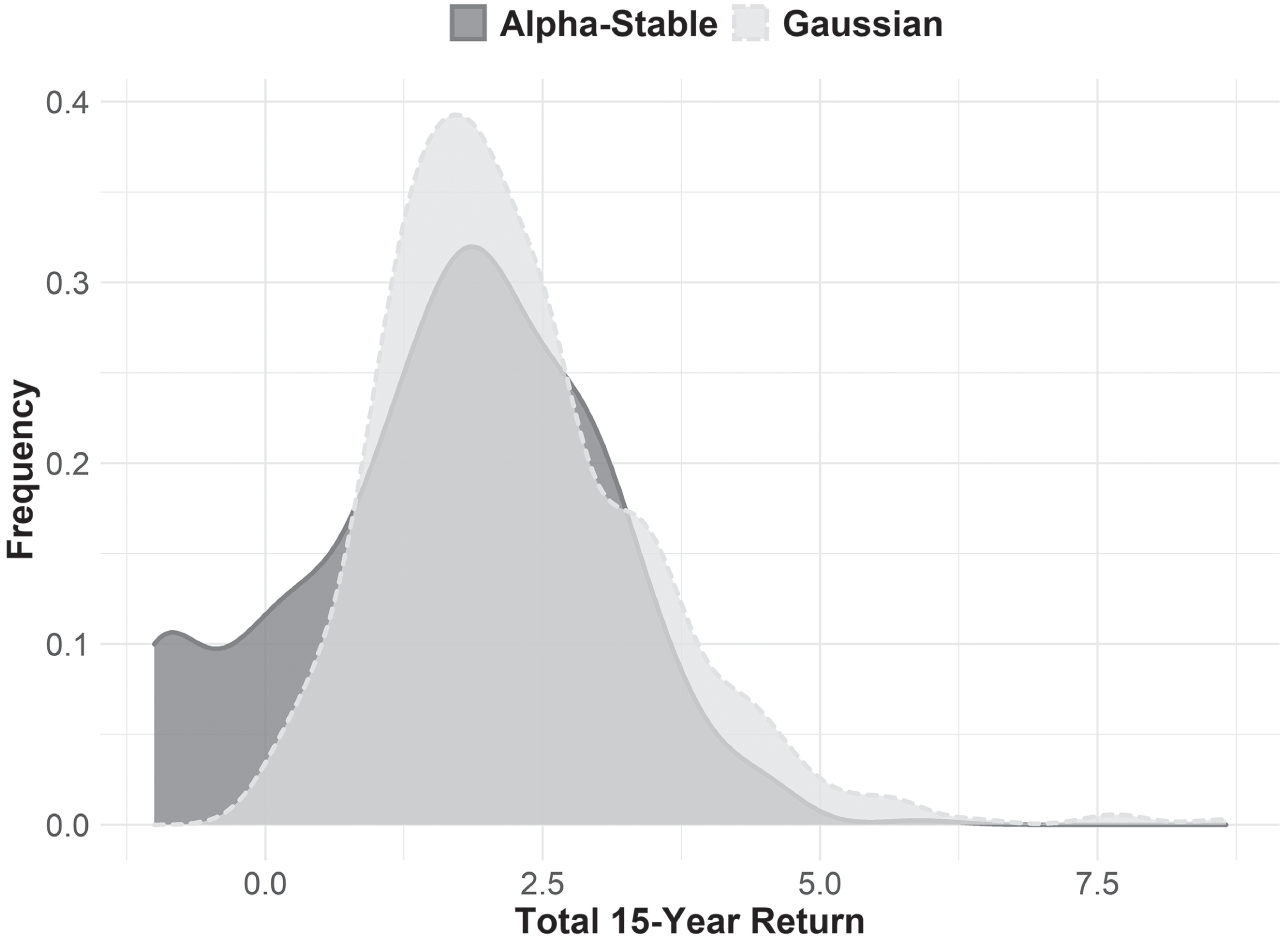
FIGURE 5.5 Simulated Cumulative Returns Drawn from the Annual Returns of Gaussian and Alpha‐Stable Distribution
Parameters calculated from the annual return of a 60% SPY, 30% AGG, 10% GLD portfolio, in the period 2004 through 2020
If returns are not Gaussian this mathematical equivalence across time goes away. As the density plot shows, 15‐year aggregate Gaussian returns cluster in a predictably normal fashion, whereas 15‐year cumulative alpha‐stable distributions cluster entirely differently (bad things happen far more often with alpha‐stable distributions, and there are fewer positive outcomes, see Figure 5.5). Of course, this is what we see in the real world, as the histogram of rolling 10‐year returns for the S&P 500 demonstrates (Figure 5.6). These aggregate returns do not cluster the way a Gaussian distribution would predict. Rather, they aggregate in a manner much more akin to an alpha‐stable distribution.
In truth, that market returns are not Gaussian is a widely known and widely studied fact. Indeed, finding methods and quantitative tools for the combination of non‐Gaussian investments into a portfolio was an early project in economics. Nobel‐laureates Eugene Fama and Paul Samuelson, as well as famed mathematician Benoit Mandelbrot,3 along with many others, attempted to find some solutions. They were met with very limited success, unfortunately. Even though the brightest minds in finance attempted to tackle the problem, we really have no practical tools to combine portfolios of alpha‐stable distributions. While we may agree that market returns are not Gaussian, abandoning that assumption leaves us with a whole new problem: We have no way to understand how weighting investments affects the parameters of the aggregate portfolio's return distribution. Clearly, this is a problem. My genuine hope is that brighter minds than mine will develop a solution in the near future. Absent that, I propose that practitioners use the Gaussian assumption to get close to the right portfolio, then use the alpha‐stable distribution parameters of the portfolio to inform risk control and the final probabilities of goal achievement. Obviously, Monte Carlo simulations based on the Gaussian assumption should be abandoned in favor of simulators based on alpha‐stable distributions—Gaussian Monte Carlo simulations can be quite dangerous and they are in very common use. Today, most platforms have libraries for both the estimation of the parameters and random‐number generation of an alpha‐stable distribution—all that is needed for a Monte Carlo simulator—so practitioners can readily upgrade their approach.
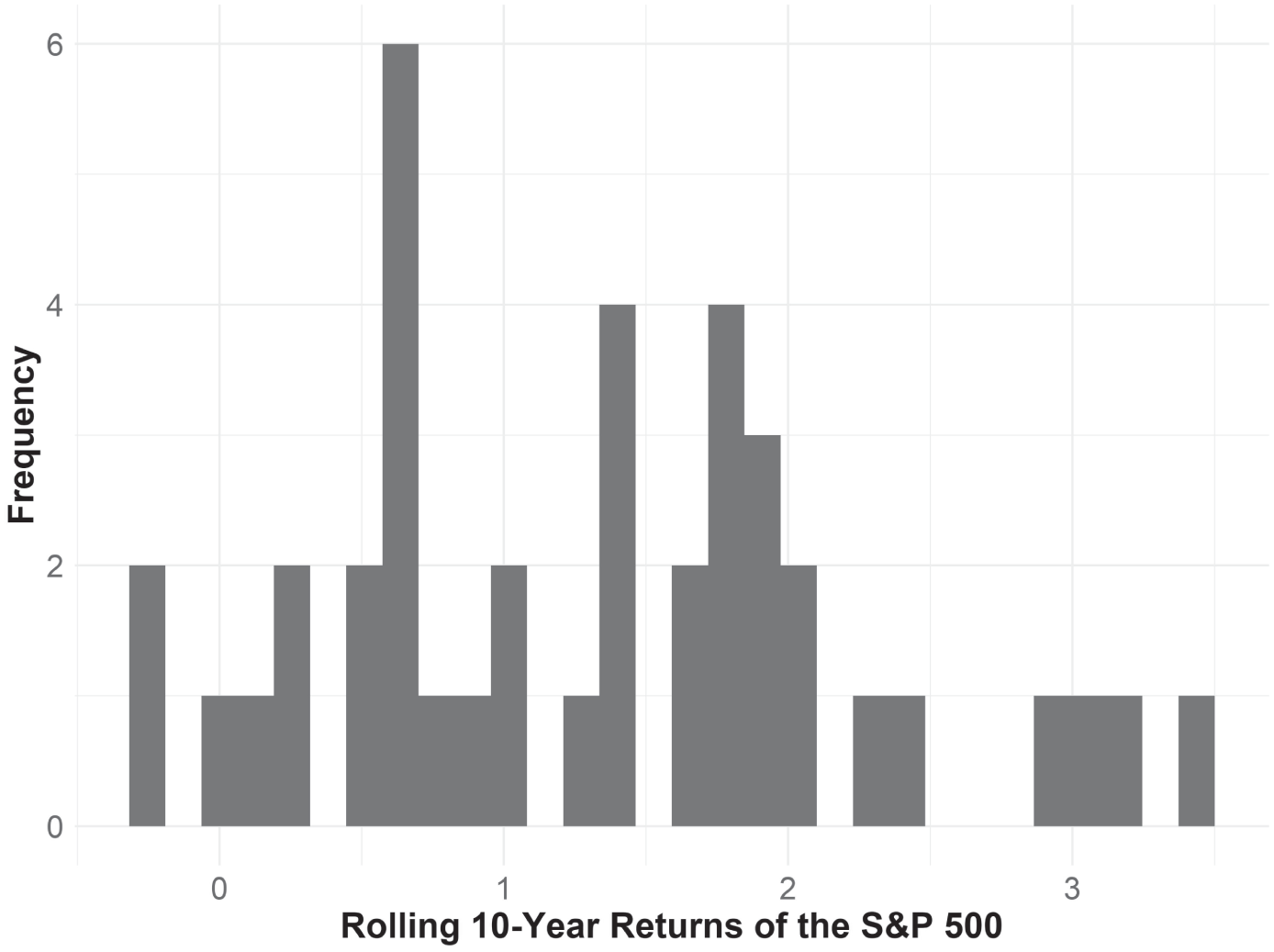
FIGURE 5.6 Rolling 10‐Year Returns of the S&P 500 Index
1970 through 2019
Downside risk control takes on added importance in a non‐Gaussian paradigm. Those of us working in the industry well know that an average return is only part of our concern, we are also concerned with when drawdowns happen, relative to the time horizon for your goal. This was the concern of my first peer‐reviewed publication. Coming out of 2008, I had a basic question: How much can you lose in an investment portfolio before you have lost too much? What I learned through difficult experience is that, while markets recover, they may not recover in time for investors to accomplish their objectives. Surprisingly, no one had yet taken up this question, so I proposed a simple rule for understanding when portfolio losses are too much to recover from.4
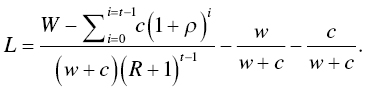
The logic runs like this. Suppose we have a bad year in our goals‐based portfolio. We now have a new and higher return requirement in the subsequent year, defined as
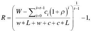
where ![]() is the future funding requirement of the goal,
is the future funding requirement of the goal, ![]() are the annual contributions to the portfolio,
are the annual contributions to the portfolio, ![]() is the time horizon of the goal,
is the time horizon of the goal, ![]() is the current wealth dedicated to the goal,
is the current wealth dedicated to the goal, ![]() is the annual growth rate of the contributions, and
is the annual growth rate of the contributions, and ![]() is the one‐year return (loss) we experience in the portfolio. Given our goal variables and a loss we might experience in the portfolio, we now have the new annual return requirement of the portfolio. Going a step further, if we have an estimate for the portfolio's return coming out of a serious loss, and let that stand in for
is the one‐year return (loss) we experience in the portfolio. Given our goal variables and a loss we might experience in the portfolio, we now have the new annual return requirement of the portfolio. Going a step further, if we have an estimate for the portfolio's return coming out of a serious loss, and let that stand in for ![]() , then we can take the equation above and solve for the maximum loss our portfolio can weather and still be reasonably expected to recover:
, then we can take the equation above and solve for the maximum loss our portfolio can weather and still be reasonably expected to recover:
What we find using this formulation is that loss tolerance is based on quite a few factors, of which time horizon is probably the most important (though recovery return, ![]() , is also key). As the time until a goal diminishes, we find that a portfolio becomes less able to weather losses, as illustrated in Figure 5.7. Again, this squares with our intuition, but is generally poo‐pooed by the academic establishment. Goals‐based investors, because of their finite time horizon, must be cognizant of the order of their returns as well as the average of those returns—and this would be true even with a Gaussian return assumption.
, is also key). As the time until a goal diminishes, we find that a portfolio becomes less able to weather losses, as illustrated in Figure 5.7. Again, this squares with our intuition, but is generally poo‐pooed by the academic establishment. Goals‐based investors, because of their finite time horizon, must be cognizant of the order of their returns as well as the average of those returns—and this would be true even with a Gaussian return assumption.
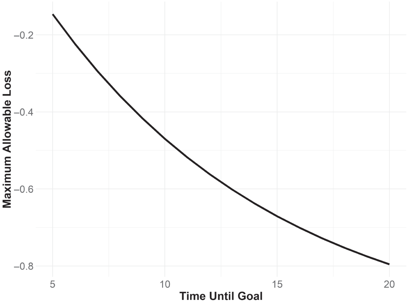
FIGURE 5.7 How Time Horizon Affects Loss Tolerance
Goal is to have $1 with $0.80 in current wealth, no contributions, and a 10% per year portfolio recovery return.
The importance of this definition of losses is that it has nothing at all to do with the investor's psychological risk tolerance. This has nothing to do with how comfortable an investor is with risk. Rather, this is an entirely quantitative definition of risk tolerance based on the objective of the portfolio (with an input for a market recovery expectation). In my own experience, I have also found that by understanding losses within the goals‐based context, investors become considerably more tolerant of losses. Investors intuitively understand that portfolio losses reduce the probability of achieving their goals, but they rarely know exactly how. That is why all losses tend to feel excessive. However, when placed in this context, investors can know rather than guess how losses affect their ability to achieve a goal, and have a plan to mitigate their risk. Losses, then, are not something to be feared—at least most of the time.
In my original research, I more‐or‐less hand‐waved away the question of how investors go about managing that risk in practice. I proposed that once maximum losses were reached (or almost reached), investors simply exit the portfolio and reinvest again next year. That is a very shallow solution (and the anonymous peer‐reviewer told me as much). Stop‐losses have their own risks to goals‐based investors. Namely, as soon as you exit a position, you have exchanged downside risk for upside risk (notice how goals‐based investors are never without some kind of risk!). Downside risk is the risk of loss, of course, but upside risk is considerably less familiar for most investors. Upside risk is the risk that you are in cash when markets start running higher, thereby leaving you without the benefit of that return. It is this upside risk that proponents of buy‐and‐hold‐forever strategies point to when clients call with a strong urge to sell, though they do not exactly call it that.
Upside risk is very real, and for long‐term goals it is usually the most acute. However, we should not completely dismiss stop‐loss strategies. Of the many risks inherent in them (and there are many), the one I usually hear is, “How do you know when to get back in?” A fair question, and this is a question we will analyze in more detail using the goals‐based lens in a moment. But even non‐goals‐based traders can answer this question satisfactorily: So long as we buy at a lower price than we exited, we come out ahead on the trade. But let's not forget, money is not a single block. We can invest some percentage of our portfolio at lower prices and begin balancing our upside risk with our downside risk.
Let's define our breakeven price as the price at which we must buy back in lest we are forced to buy at a price higher than our exit (and thereby lose money on that trade). For example, if we exited our entire portfolio at $100/share, then we must buy back in at a price below $100/share to break even. However, if we account for partial buys, then our breakeven price is defined as:
where %Invested is the percentage of the portfolio (or position) that was reinvested at the Price Invested. If we instead know the new breakeven price we would like to have, we can apply some algebra and learn what percentage we need to invest at a given price to attain our desired breakeven price:
Upcoming losses can also be understood in terms of %Invested:
where the Loss to Go is the amount of losses still expected to come in the position (or portfolio).
With this basic framework, a portfolio manager (or trader) with even some insight on markets can then balance downside risk with upside risk. Clearly, there comes a point where upside risk (simply defined as “losing money by buying above our exit point”) outweighs downside risk, and vice versa. The point here is not that this basic framework is a panacea for “when should you get back in,” but rather, that there is a framework for answering such a question, assuming the practitioner has even a very basic view on capital markets.5
My original thoughts on defining maximum allowable losses also led to some interesting discussions around the various quantitative factors affecting loss tolerance.6 Figure 5.7 demonstrates how time horizon affects loss tolerance—showing clearly that losses become less tolerable as the goal approaches (a result we have all known intuitively, though have not been able to quantify). Borrowing the language of options, we could say that this is a form of theta risk, of time decay. However, movements in portfolio value also affect loss tolerance—a form of delta risk. As the portfolio gains in value, loss tolerance increases, and as the portfolio loses in value, loss tolerance decreases, as can been seen in Figure 5.8. There are several other “Greeks” that may well apply to loss tolerance, such as gamma risk, rho, and even a form of duration. Suffice it to say, there is quite a lot going on here, but I fear I have digressed too far as it is, so I will simply direct interested readers to my paper on the subject.7
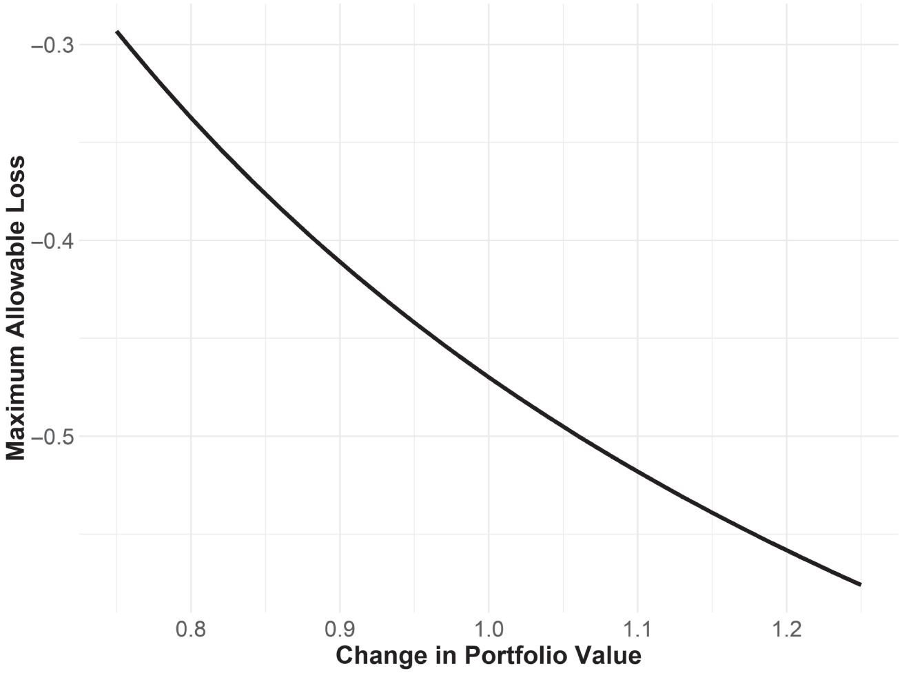
FIGURE 5.8 How Changes in Portfolio Value Affects Loss Tolerance
Goal is to have $1 in in 10 years, with $0.80 in current wealth, no portfolio contributions, and a 10% per year portfolio recovery return.
TABLE 5.1 Allocation of Example Investors
| SPY | AGG | |
|---|---|---|
| John | 100% | 0% |
| Alice | 14% | 86% |
| Pamela | 80% | 20% |
Still yet another way to think about portfolio movements in the context of goal achievement—and a helpful way to illustrate why investors worry about portfolio losses—is to look at portfolio movements through the lens of goal achievement probability. That is how goals‐based investors feel markets, so it can be helpful to see portfolio movements through their eyes.
To do this, let us take three example investors and their goals. John, our first investor, needs $1 in 15 years to retire comfortably. This is a priority goal (so its value is coded as 1.00). He currently has $0.32 dedicated to this goal, and he expects to get 10% returns per year from a portfolio with volatility of 18% over that 15‐year period. Alice, our second investor, needs to have $1 in four years to send her child to college, and she currently has $0.95 saved. She expects to get 4% per year from a portfolio with around 9% volatility, and this goal has a value of 0.75. Lastly, we have Pamela. Pamela needs $1 in eight years to fund a bequest for which she has $0.65 today, and she values this goal at 0.22. Pamela expects to generate 7% per year from a portfolio that carries about 16% volatility. Finally, let us suppose that each of our investors is allocated between SPY (the SPDR S&P 500 ETF) and AGG (the SPDR US Aggregate Bond Index ETF), according to Table 5.1.
The plots illustrate how each investor experienced 2020. As practitioners, we are tempted to focus on Panel A of Figure 5.9, which shows the change in portfolio value for each investor from their starting position. John and Pamela, we might be tempted to conclude, were happiest with our work in the end, as they had the largest gain in portfolio value. However, portfolio value is not how goals‐based investors experience markets! Figure 5.9, Panel B, demonstrates how our investors “felt” their portfolio movements through 2020. Alice was happiest with our work because, as it turns out, she saw the largest gain in her goal achievement probability, and those gains accrued to a valuable goal. John was a distant second! Despite having the largest return, he did not experience much change in achievement probability, and the downturn was quite damaging. Even more counterintuitive: During the market bottom, we might have thought that Alice would be happiest with our work as she lost the least money, but it was actually Pamela who saw the smallest change in utility. Pamela, not Alice, was happiest with how we handled the downturn, despite the former losing 25% and the latter losing only 7.5%! I can imagine a befuddled portfolio manager attempting to navigate this conversation without a goals‐based perspective!
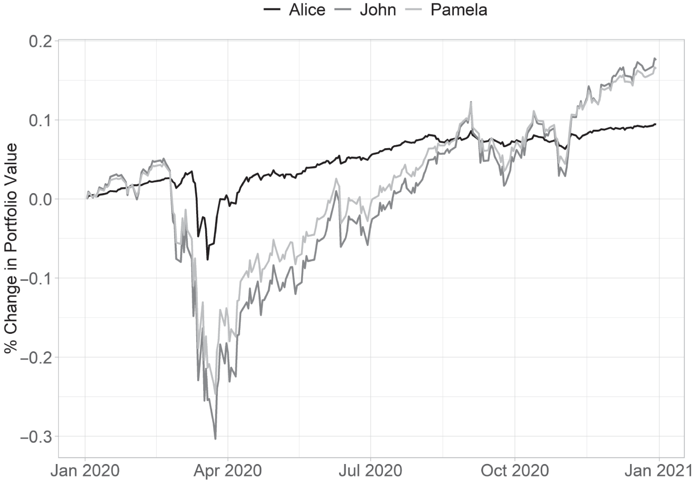
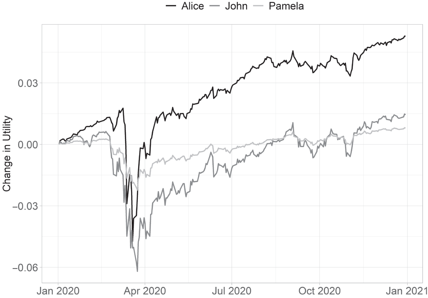
FIGURE 5.9 Example Investors' Experience of 2020
Panel A: Change in Portfolio Value, Relative to the Start of 2020
Panel B: Change in Goals‐Based Utility, Relative to the Start of 2020
Daily probability of achievement times goal value, relative to the start of 2020.
As becomes quite clear in this example, how an investor experiences portfolio movement has as much to do with what investors are trying to achieve—and their current progress in achieving it—as how the portfolio behaves relative to a starting point or a benchmark. Indeed, one might excuse Alice for being upset in the depth of the selloff, since she lost 5.5% points of achievement probability (though she ended the year up almost six percentage points).8 Practitioners who focus on the statement value are not speaking the language of their investor, assuming that investor has some goals she is trying to achieve with the funds. Changes in portfolio value should always be contextualized and understood through the lens of goal achievement.
And this example also illuminates the larger point: Losses do matter to goals‐based investors, confirming our intuition on the subject,9 but how much they matter is highly individualized. While simplistic stop‐loss strategies (like the one I offered in my paper as a hand‐wavy solution) carry risks that are not accounted for in the example model, investors could turn to more sophisticated strategies, such as hedging. With hedging, the follow‐up question to “Investors should protect their downside risk” is, “What are you willing to pay for that protection?” As with everything, we must make tradeoffs. Protecting against excessive losses must be weighed against the cost of doing so. In practice, the most accurate solution to this question would be to include a hedge in a multiperiod optimizer, like the one offered in the previous chapter. Rather than leave it at that, and in an effort to build our intuition on the topic, let's push forward our logic from above to get a sense of what the fair value of a hedge might be to a particular portfolio.
There are four basic outcomes with which we are concerned when hedging. We could pay for a hedge in the portfolio and the market downturn does not happen for the duration of the hedge. In that scenario, we are out the cost of the hedge, and the portfolio must carry a slightly higher return than it otherwise would have to maintain the same goal achievement probability. Let's call that return scenario ![]() , and our updated return requirement is
, and our updated return requirement is ![]() , where
, where ![]() is the cost of the hedge and
is the cost of the hedge and ![]() is the return harvested by the portfolio in a typical year. Of course, we could pay for the hedge and the bad year happens—we bought a hedge and it paid off. Let's call that
is the return harvested by the portfolio in a typical year. Of course, we could pay for the hedge and the bad year happens—we bought a hedge and it paid off. Let's call that ![]() . In that scenario, we have incurred the cost of the hedge, but our portfolio loss is offset by the benefit of the hedge. For convenience, let's just say that
. In that scenario, we have incurred the cost of the hedge, but our portfolio loss is offset by the benefit of the hedge. For convenience, let's just say that ![]() is the return of the portfolio when hedged in a bad year, so
is the return of the portfolio when hedged in a bad year, so ![]() .
.
We could choose to not hedge the portfolio. We may not get a bad year, so let's call that return outcome ![]() , and
, and ![]() . Note that we get the same portfolio return as
. Note that we get the same portfolio return as ![]() , except there is no hedge cost. Finally, we could choose not to hedge and the loss happens anyway. Let's dub that return scenario
, except there is no hedge cost. Finally, we could choose not to hedge and the loss happens anyway. Let's dub that return scenario ![]() , and
, and ![]() . And, of course, we have a market view. Let
. And, of course, we have a market view. Let ![]() be the probability of a bad year occurring, leaving
be the probability of a bad year occurring, leaving ![]() as the probability of a typical market year. These return scenarios are laid out in Table 5.2.
as the probability of a typical market year. These return scenarios are laid out in Table 5.2.
Now with the details ironed out, we can set up the problem. We are concerned with when the benefits of hedging are equal to the nonhedged scenario. As always with goals‐based portfolios, we are using probabilities to measure benefit. We are, then, concerned with the truthiness of
In these formulations, we will need to input a recovery return and recovery volatility expectation for the portfolio in the ![]() functions for the hedged‐and‐loss (
functions for the hedged‐and‐loss (![]() ) and not‐hedged‐and‐loss (
) and not‐hedged‐and‐loss (![]() ) scenarios, and a more typical return and volatility profile for the hedged‐and‐no‐loss (
) scenarios, and a more typical return and volatility profile for the hedged‐and‐no‐loss (![]() ) and not‐hedged‐and‐no‐loss (
) and not‐hedged‐and‐no‐loss (![]() ) return scenarios. Unfortunately, because the cost variable shows up in two places, there is not an easy algebraic solution, but we can use an optimizer to help us find the hedge cost that makes the above equation true.
) return scenarios. Unfortunately, because the cost variable shows up in two places, there is not an easy algebraic solution, but we can use an optimizer to help us find the hedge cost that makes the above equation true.
Let us consider an illustration. In Figure 5.10, we see how our outlook for the probability of a loss scenario in the coming year affects how much we are willing to pay to hedge the portfolio. In all of the illustrated scenarios, the required future value is $1.00. In Scenario A, our client has $0.75 dedicated to the goal, a time horizon of 10 years, and we expect a bad year to deliver a loss of 40%. By paying for the hedge in Scenario A, we expect to incur a loss of 25% (plus the cost of the hedge, of course). When we see a 50% probability of a 40% loss, given these figures, we are willing to pay up to $0.09 to bring that loss down to 25%. Of course, an investor would rather pay less for the hedge, if possible; this is a maximum. A more traditional view might put the fair value of the hedge around its expected value, or the amount of money it saves times the probability of that savings: ![]() . However, the more nuanced goals‐based perspective shows us that the hedge is in fact worth more to this investor, and the investor then has more pricing power.
. However, the more nuanced goals‐based perspective shows us that the hedge is in fact worth more to this investor, and the investor then has more pricing power.
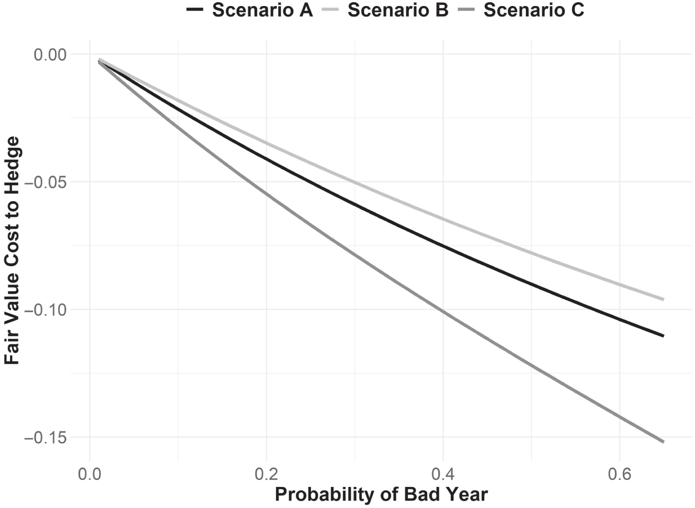
FIGURE 5.10 Effect of Loss Probability on Hedge Fair Value
For all scenarios, the expected portfolio return in a typical year is 8% with a volatility of 11%, and the expected portfolio return after a loss year is 10% with a volatility of 9%. Return distributions are assumed logistic.
Scenario B changes the expected portfolio loss without the hedge to 30% and the hedged loss expectation to 15%. Note here that, in terms of dollar value, the net benefit of the hedge is the same as Scenario A. In both scenarios we are protecting 15% of portfolio value, yet in Scenario B our investor is not willing to pay as much for a hedge. Recall, the probability of goal achievement drops exponentially with losses because they make it ever more difficult to achieve the necessary recovery return. Sensibly, then, the benefits of hedging also grow exponentially. It is not just the net dollar benefit of the hedge with which we are concerned; we are also concerned with where that protection falls on the loss spectrum. Indeed, investors may well be willing to pay a higher price to offset the last 10% points of a 60% loss than they would be to offset the last 10 percentage points of a 15% loss, a puzzling result to traditional theory.
Scenario D shifts the time horizon down to 5 years instead of 10 years, as it was in the previous two scenarios. In addition, Scenario D ups the benefit of the hedge. Without the hedge, we expect a loss of 40%, but with it we can trim that loss down to 15%. Willingness to pay for the hedge grows considerably faster than in the previous scenarios, largely because the time to regain lost ground is much lower.
I want to draw your attention to something very different about this view of hedging costs. This model is heavily driven by goal variables, meaning every investor will have a different fair value hedging cost. What's more, every portfolio for every investor is very likely to have a different fair value hedging cost, depending on the goal to which it is dedicated. Fair value is defined as much by you and your goals as it is defined by how markets work. I am aware of no other derivative pricing model that individualizes pricing like this. Of course, this has implications for how derivative markets discover price, but I will address some ideas of goals‐based market pricing in a later chapter.
As I mentioned above, willingness to hedge should be an asset allocation decision made within the context of a multiperiod framework, as described in the previous chapter. Even so, I wanted to build our intuition around risk management in a goals‐based context, as it is different than the more traditional view. I also find it immensely interesting that hedge pricing is dependent not just on our view of markets, as normative theory suggests, but also on our goal variables. Of course, every firm has a unique risk management philosophy, so my purpose here is not to convince you to adopt a different one. Rather, as I have discussed before, we practitioners cannot do our job without first understanding the job that needs doing. Where risk management should be done, it should be done in a goals‐based context, just like everything else we do for clients. Goals‐based investing really is at the intersection of markets and people. Goals‐based risk management is no different.
If anything, the mere understanding that markets are quasi‐wild horses rather than reliable tractors should be a benefit to clients. After all, it is them, much more than us, who get kicked in the teeth when things go wrong. In such a model of the world, the timing and severity of losses matters! We cannot manage these risks if we do not acknowledge them, and a key outcome of goals‐based portfolio theory is to at least acknowledge them. How practitioners go about managing these risks is where real value is added, and I would expect that every firm will have its own approach. Outflowing from this discussion is an understanding that hedge pricing is dependent, not just on our belief about markets (i.e. the selection of the correct return distribution), but as much on the goal our investor is trying to achieve. This gives practitioners an entirely different approach to pricing portfolio hedges and managing risk than more traditional theory would suggest.
Risk management, like everything in goals‐based portfolio theory, is individualized.
Notes
- 1 Wittgenstein asked whether you were using the ruler to measure the table or the table to measure the ruler. C.f. N.N. Taleb, Statistical Consequences of Fat Tails: Real World Preasymptotics, Epistemology, and Applications (Stem Academic Press, 2020).
- 2 J. Voss, “Fact File: Sigma Events,” Enterprising Investor Blog.
- 3 E. Fama, “Mandelbrot and the Stable Paretian Hypothesis” The Journal of Business 36, no. 4 (1963): 420–429; E. Fama and R. Roll, “Some Properties of Symmetric Stable Distributions,” Journal of the American Statistical Association 63, no. 323 (1968): 817–836; E. Fama, “Risk, Return, and Equilibrium,” Journal of Political Economy 79, no. 1 (1971): 30–55; P. Samuelson, “Efficient Portfolio Selection for Pareto‐Levy Investments,” Journal of Financial and Quantitative Analysis 2, no. 2 (1967): 107–122; B. Mandelbrot, “The Variation of Certain Speculative Prices,” The Journal of Business 36, no. 4 (1963): 394–419; B. Mandelbrot, “New Methods in Statistical Economics,” The Journal of Political Economy 71, no. 5 (1963): 421–440.
- 4 F.J. Parker, “Quantifying Downside Risk in Goal‐Based Portfolios,” Journal of Wealth Management 17, no. 3 (2014): 68–77, DOI:
https://doi.org/10.3905/jwm.2014.17.3.068; F.J. Parker, “The Erosion of Portfolio Loss Tolerance over Time: Defining, Defending, and Discussing,” Journal of Wealth Management 19, no. 2 (2016): 23–31, DOI:https://doi.org/10.3905/jwm.2016.19.2.023. - 5 Any active strategy will introduce active risk to a portfolio. Whether that risk—when evaluated in light of portfolio manager skill—is an acceptable one is another matter!
- 6 I am indebted to the anonymous peer‐reviewer for this observation, which prompted the subsequent exploration. While I admit there may be little practical application, I do believe that explorations such as this are what build practitioner intuition.
- 7 F.J. Parker, “The Erosion of Portfolio Loss Tolerance over Time: Defining, Defending, and Discussing,” Journal of Wealth Management 19, no. 2 (2016): 23–31, DOI:
https://doi.org/10.3905/jwm.2016.19.2.023. - 8 This is not in the plot. I am here citing only half of the utility conversation, the probability of achievement.
- 9 I would also direct readers to Tail Risk Hedging by Vineer Bhansali, who more‐or‐less argues that investors should always be hedged, and proposes some simple rules for cashing them in. His idea is that investors can actually take on more volatility in their portfolio than they otherwise would, then hedge‐away that excess volatility. The difference between the hedge cost and the added return yields a portfolio with more return for the same amount of volatility. While not a goals‐based solution, it is an intriguing idea, and his approach certainly has relevance to goals‐based investors who are concerned with losses.