CHAPTER 2
A Theoretical Foundation
“There is nothing more practical than a good theory.”
—Kurt Lewin
I think of theory like a map. A map is not reality, of course, but a good map can lead you to your destination much more readily than a bad one. In some cases, the map is accurate but not detailed. We call that a heuristic (or rule‐of‐thumb). A heuristic works because it is picking up some underlying truth, even though the justification for it may be wrong. Sometimes the map is mostly right, but is wrong in the details. We might be able to use it to get a sense of where we are going, but we may just as easily wind up lost. In other cases, the map is simply wrong, rendering it useless. In that case, we have to throw the map away, explore the unknown area, and draw a new map. As I have witnessed in my own practice, poor theory can lead to poor practical outcomes, but it is not enough to simply decry the map altogether. We must understand why the map is leading us astray. Is it entirely wrong? Or is it simply that the map is not detailed enough? Understanding where and why the map is wrong is an important component to drawing a new one! In my view, traditional portfolio theory is not an entirely useless map (though it is popular to paint it as such). Rather, it is a map that is mostly right some of the time, but often wrong in the details. I see current portfolio theory like one of those early post‐Columbian maps showing that North America exists, but not in a way that helps you actually get to North America—the islands and dangerous shoals are not marked, and neither is the shoreline accurately reproduced. The purpose of this chapter is to fill in those details that help us actually get to where we want to be.
Like most models of choice, we must begin with John von Neumann and Oskar Morgenstern's axioms of rational choice.1 In short, they find that any rational decisions must be consistent with four basic axioms:
- Complete. For any choices, you must be indifferent to them or prefer one to the other. In other words, you must be able to order your preferences.
- Transitive. For any choices, if you prefer A to B and you prefer B to C, then you must also prefer A to C.
- Continuous. For any choices, there is some factor of your most‐liked and most‐disliked that you can incorporate to make you indifferent to the middle option. In other words, if you prefer A to B to C, then there exits some number,
 , such that you are indifferent to getting
  and
and  , or getting
  by itself.
 - Independent. For any choices, adding some random third choice does not affect your preference. If you prefer A to B, you should still prefer getting A and C to B and C.
I do not think it is an exaggeration to say that von Neumann and Morgenstern's (hereafter I'll call them VNM) axioms of rational choice were responsible for sparking the behavioral economics revolution. Not even a decade after VNM's publication, Maurice Allais presented the results of an experiment2 in which he showed that people tend to disregard the axiom of independence (Axiom D above). Allais's conclusion was that if reasonable people deciding between simple alternatives contradicted the axiom, then the axiom was a poor one. In his monumental 1959 book Portfolio Selection, Markowitz3 retorted that “individuals choosing the ‘wrong' alternative acted irrationally.” And so, the normative‐behavioral split was formed. Interestingly, because Allais relies on changes in probabilities, his experiment can also be solved if people do not perceive probabilities objectively. That is, if people feel the shift from, say, a 90% probability of success to a 95% probability of success more than they feel the shift from a 10% to a 15% probability of success, then Allais's results can be explained without the abandonment of the axiom of independence, but this, of course, creates a whole different set of problems with rationality.4
This is relevant because we must acknowledge what it is we are attempting to do when constructing our goals‐based map. Behavioral finance is concerned with a descriptive theory of behavior—that is, how do people actually behave. Normative finance is concerned with a prescriptive theory of behavior—how people should behave. While I acknowledge the role of managing client (and our own!) irrationality, it is my objective to build a normative theory for goals‐based investors. We want to know what the rational course of action is, even if we later decide to modify it to accommodate behavioral concerns. What's more—and this is the topic of a later chapter—when viewed through the lens of goals‐based theory, it may be that individuals are not as irrational as normative finance makes it seem. Numerous behavioral‐normative puzzles resolve themselves when we simply account for what it is individuals are attempting to do. In this way, goals‐based portfolio theory may well provide a bridge across the chasm formed between normative and behavioral economics, and that is quite exciting to me!
Accepting that VNM's axioms are indeed a structure for making rational choices (and not just between lotteries as they originally indicated, but between any types of things), we will accept them and add one more: we will assume that individuals prefer a higher probability of achieving their goal than less. In the language of VNM:
- Attainment. If you prefer having
 to not having
  , then you should prefer
  to
to  when
when  , you should be indifferent to
  or
or  when
when  , and you should prefer
  to
to  when
when  .
.
Thus, using these five simple axioms, we can build a theory for the rational allocation of wealth to investments (i.e. portfolio construction) and the allocation of wealth across goals.
Before we press forward, however, I want to clarify why starting from these basic axioms is important. Most people are well aware of the portfolio construction problem—how to allocate wealth across investments—as this has been widely discussed and practiced for decades. Constructing an investment portfolio is a question of allocating within goals. The allocation across goals, however, is a separate problem that has been given very little discussion in the literature. Until recently, it has been simply assumed that individuals have already allocated their wealth across their various goals appropriately. I would like to camp here for just a moment to clarify the problem so that the solution makes more sense.
People have more than one goal—this should be no big surprise. For example, suppose I want to retire in about 25 years. I also want to send my kids to college in eight years, and possibly buy a vacation home in five years. If I allocate some of my savings toward the vacation home, I necessarily reduce the probability of retiring and sending my kids to college. When I spend my limited resources on one goal, I reduce the probability of achieving my other goals. How, then, should I allocate my limited pool of wealth (existing savings as well as my future savings) in a rational manner? To date, the solution has been to engage in an iterative conversation with a financial planner. Effectively, we arrive at a proper allocation to goals by trial‐and‐error, presenting alternate probability of achievement scenarios for the various goals until the client says, “Yes, that is the right balance.” Of course, I do not advocate for the abandonment of client conversation, but this iterative approach is demonstrative of the bigger problem: we have no theoretical basis for a solution. That is, we literally do not know how to rationally allocate across goals, we rely on a hedonic solution—on client feedback—and hope that it is rational enough. In this regard, surely a map is better than no map?
To be fair, the general solution in the literature has been to acknowledge a Maslowian hierarchy of goal allocation (Figure 2.1). In his book, Brunel5 suggests that individuals will ensure they have funded their needs with a high probability of success, only then will they fund their wants and once those have been funded with a sufficiently high probability, investors will then seek to fund their wishes and dreams. This was also the perspective that Chhabra6 took in his seminal work, and Statman suggests a similar framework.7 Deguest, Martellini, and Milhau,8 building on the work of Chhabra, propose a more formalized idea: investors will allocate such that their essential goals are met for sure, and then divide wealth across goals that cannot be achieved for sure. While I agree with many of the elements from these frameworks, all of this is rather ad hoc, and none of the frameworks offer a complete and cohesive solution. More important to me is that none of these solutions can be properly called rational because they have no fundamental mathematical and logical basis. Of course, I want to ensure that I can eat in 25 years, but how much loss of achievement probability in my retirement goal am I willing to stomach to see my children graduate college with little to no debt? In each of the frameworks so far, the practitioner must return to the investor to ascertain the final answers, but that assumes the investor will make a rational decision! Again, I do not advocate for the abandonment of client conversation, but I believe there is a quantitative answer lurking beneath this very human problem.

FIGURE 2.1 Maslow‐Brunel Hierarchy of Goals
This subject carries an additional nuance in goals‐based portfolio theory. Among the other goals people set, most people have aspirational goals—goals they would like to achieve but realize that their achievement is unlikely (the “dreams” category in the Maslow‐Brunel pyramid). Traditional finance likes to pretend these aspirational goals do not exist, preferring to just constrain them away.9 Yet we know such goals exist, and an ability to rationally allocate across goals, including aspirational goals, allows us to declare a budget for these considerably more aggressive goals. As we shall see, it may be rational to gamble at times, but certainly not to gamble everything.10 By including the allocation of wealth across goals in the theory, we can now confidently say when someone is behaving irrationally with respect to their own aspirations. We can also confidently say how much achievement probability of retiring our client is willing to sacrifice to gain that aspirational goal.
With these preliminaries now out of the way, let us press ahead with the technical details.
We assume that people set multiple goals, and that these goals compete for a “single” pool of wealth, which we will call ![]() . This pool of wealth is the sum of all financial assets plus the discounted value of all future savings (i.e. financial capital and human capital). Of course, in practice, this pool of wealth is going to have real‐world frictions that matter to our model, but for now we will disregard those to be revisited later. We will refer to this set of goals as the goals‐space, or
. This pool of wealth is the sum of all financial assets plus the discounted value of all future savings (i.e. financial capital and human capital). Of course, in practice, this pool of wealth is going to have real‐world frictions that matter to our model, but for now we will disregard those to be revisited later. We will refer to this set of goals as the goals‐space, or ![]() , where
, where ![]() are the N‐number of goals in the goals‐space.
are the N‐number of goals in the goals‐space.
The axiom of completeness means that we can rank‐order the goals, so we will let ![]() represent the most favored goal,
represent the most favored goal, ![]() represent the second‐most favored goal, and so on. For ease of mathematical discussion, let there be a value function of the goals,
represent the second‐most favored goal, and so on. For ease of mathematical discussion, let there be a value function of the goals, ![]() , such that
, such that ![]() if
if ![]() is preferred to
is preferred to ![]() ;
; ![]() if you are indifferent to
if you are indifferent to ![]() and
and ![]() ; and
; and ![]() if you prefer
if you prefer ![]() to
to ![]() . Since all of this is a mathematical construct, let us simply say that
. Since all of this is a mathematical construct, let us simply say that ![]() is always the most valued,
is always the most valued, ![]() is always the second‐most valued, and so on. The convenience of
is always the second‐most valued, and so on. The convenience of ![]() and the axiom of continuousness allows us to say that some number exists,
and the axiom of continuousness allows us to say that some number exists, ![]() , such that
, such that ![]() .
.
Here we have reached an important point. That we can reduce the value of ![]() sufficiently to make the choice equivalent to
sufficiently to make the choice equivalent to ![]() means we can ascertain the value of
means we can ascertain the value of ![]() relative to
relative to ![]() using a certainty equivalence method. This involves assigning an arbitrary number to
using a certainty equivalence method. This involves assigning an arbitrary number to ![]() . I like using
. I like using ![]() (though any positive real number would do11). From there, we can ask whether you would prefer achieving
(though any positive real number would do11). From there, we can ask whether you would prefer achieving ![]() with certainty or achieving
with certainty or achieving ![]() with probability
with probability ![]() . By varying
. By varying ![]() until you are indifferent to the choice, we can then infer that
until you are indifferent to the choice, we can then infer that ![]() , or that
, or that ![]() is only
is only ![]() as valuable as
as valuable as ![]() .
.
Again, for convenience, let us create a new set of variables to hold these newly formed value ratios. As is my preference, ![]() , so
, so ![]() .
. ![]() , then, would be
, then, would be ![]() . By repeating the certainty equivalence procedure across the goals‐space, we can map these value ratios to the goals‐space,
. By repeating the certainty equivalence procedure across the goals‐space, we can map these value ratios to the goals‐space, ![]() , and the total value, then, of the goals‐space is
, and the total value, then, of the goals‐space is
I think a “for instance” is appropriate here. Suppose an investor has four goals in her goals‐space, which she has rank‐ordered, ![]() . We now ask her the series of questions:
. We now ask her the series of questions:
- Would you rather achieve goal B with certainty or goal A with probability p?
- Would you rather achieve goal C with certainty or goal B with probability q?
- Would you rather achieve goal D with certainty with certainty or goal C with probability z?
As mentioned, we vary p, q, and z until our investor is indifferent to the choices. Since we arbitrarily set ![]() , we now have value ratios that correspond one‐for‐one to the goals‐space:
, we now have value ratios that correspond one‐for‐one to the goals‐space: ![]() . It is important to remember that these value ratios are not the actual values that go into the model! There is one more step to get the goal values. The value of a goal is the product of the goal ratios that precede it in the ranked order. So,
. It is important to remember that these value ratios are not the actual values that go into the model! There is one more step to get the goal values. The value of a goal is the product of the goal ratios that precede it in the ranked order. So,
Of course, goals‐based investors are investing because they do not currently have enough financial wealth to achieve all of their goals (if they did, then they would just apply the wealth to accomplish the goal). Furthermore, we assume there is some distribution of returns function that describes the investment portfolio (it need not be Gaussian!). If we let ![]() and
and ![]() represent the initial wealth we dedicate to a goal, the final wealth amount that is required to achieve the goal, and the time horizon within which the goal is to be accomplished, respectively, then we can say that some cumulative distribution function exists that takes in these goal inputs and investment portfolio weights, and returns the probability of achieving the given goal:
represent the initial wealth we dedicate to a goal, the final wealth amount that is required to achieve the goal, and the time horizon within which the goal is to be accomplished, respectively, then we can say that some cumulative distribution function exists that takes in these goal inputs and investment portfolio weights, and returns the probability of achieving the given goal: ![]() . We can alternately describe the initial wealth dedicated to a goal as some percentage of the total wealth pool owned by our investor. Let
. We can alternately describe the initial wealth dedicated to a goal as some percentage of the total wealth pool owned by our investor. Let ![]() be the percentage of the total wealth our investor allocates to a given goal, and let us call our total wealth pool
be the percentage of the total wealth our investor allocates to a given goal, and let us call our total wealth pool ![]() . Because
. Because ![]() , our probability of goal achievement function now takes the form
, our probability of goal achievement function now takes the form ![]() .
.
Lastly, we learn from Markowitz that the weighted‐sum formulation of utility is a valid solution to VNM's axioms of choice:12
where the range of possible outcomes is indexed with ![]() ,
, ![]() is the value of the ith outcome, and
is the value of the ith outcome, and ![]() is the probability the ith outcome. We can translate this solution into our context. As we have learned, each goal has its own value and its own probability of achievement based on the portfolio we choose and the relevant variables (time horizon, initial wealth, and required funding wealth). So, we can replace
is the probability the ith outcome. We can translate this solution into our context. As we have learned, each goal has its own value and its own probability of achievement based on the portfolio we choose and the relevant variables (time horizon, initial wealth, and required funding wealth). So, we can replace ![]() with our probability of achievement function,
with our probability of achievement function, ![]() , and replace
, and replace ![]() with the value of each goal in our goals‐space.
with the value of each goal in our goals‐space.
By varying how much wealth we allocate to a particular goal (![]() from above), and by controlling the weights of investments within each goal (let
from above), and by controlling the weights of investments within each goal (let ![]() represent those weights), we can maximize our investor's well‐being:
represent those weights), we can maximize our investor's well‐being:
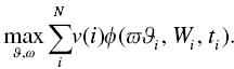
In this form, we have indexed the goals‐space with ![]() , so we are trying to maximize the sumproduct of the probability of achievement of goals
, so we are trying to maximize the sumproduct of the probability of achievement of goals ![]() through
through ![]() and the value of goals
and the value of goals ![]() through
through ![]() . Notice how the allocation of the total wealth pool, the required funding level, and the time horizon are all indexed. That is because those variables are unique to each goal, and those variables are given by the client. The allocation to each goal (
. Notice how the allocation of the total wealth pool, the required funding level, and the time horizon are all indexed. That is because those variables are unique to each goal, and those variables are given by the client. The allocation to each goal (![]() ) and the weight of each investment (
) and the weight of each investment (![]() ) are determined by an optimizer.
) are determined by an optimizer.
![]() can be any function that takes the goal variables and portfolio weights as inputs and returns the probability of achieving the goal as its output. I say any function and choose not to be too specific here because the assumption of a Gaussian distribution of market returns is, by far, the most common in the literature, but it is also the least realistic. Practitioners should be concerned with a real‐world model for asset returns because, I have said before and will say again, goals‐based portfolio theory is about achieving goals given real‐world constraints. It would be convenient if markets produced Gaussian distributions, but they do not. Therefore, in my view, non‐Gaussian distributions are one of those real‐world constraints. I will leave the rest of that discussion for a later chapter.
can be any function that takes the goal variables and portfolio weights as inputs and returns the probability of achieving the goal as its output. I say any function and choose not to be too specific here because the assumption of a Gaussian distribution of market returns is, by far, the most common in the literature, but it is also the least realistic. Practitioners should be concerned with a real‐world model for asset returns because, I have said before and will say again, goals‐based portfolio theory is about achieving goals given real‐world constraints. It would be convenient if markets produced Gaussian distributions, but they do not. Therefore, in my view, non‐Gaussian distributions are one of those real‐world constraints. I will leave the rest of that discussion for a later chapter.
It is important to note that this model does not account for how people go about setting goals, it just assumes that they are set. This is a problem, and I believe that some model of goal creation is important and is likely to explain a lot. The goals‐based utility model clearly shows that more goals yield more utility—up to a point. We can expect, based on the model, for individuals to fill their goals‐space up to the point where the next goal would result in lowered utility. Since each goal requires some allocation of resources, if adding another goal would pull enough resources so as to lower the probability of achieving more important goals more than it would yield big enough probability gains to less important goals, then our investor will not add that goal to her goals‐space. Consequently, windfalls, for example, would not necessarily be viewed through the lens of existing goals; rather, an investor will likely form new goals and dedicate the windfall to them (at least in part). Most laboratory economic studies that make offers of money to individuals, whether real or imaginary, are likely to be skewed by this windfall effect of goal formation. At the moment, we will have to accept this hole in the theory and hope that future research reveals a solution!
And that is pretty much the basic theory.
COMPARISON TO MODERN PORTFOLIO THEORY
While Markowitz's work in the 1950s is often cited as the foundation, modern portfolio theory (MPT) was built by numerous authors (many of whom won Nobel prizes) over the course of two decades. It seems to be a rite of passage for practitioners to level endless criticisms at MPT. However, and despite my own criticisms of the theory, I cannot stress enough how important the ideas of MPT have been to investors! More than anything, MPT gave investors a cohesive framework—a language—within which discussions of portfolio construction were possible. Prior to MPT, portfolio construction was an ad‐hoc affair, the aggregate result of many small decisions. The Intelligent Investor, Benjamin Graham's magnum opus on value investing, for example, has no discussion of how securities should interact within a portfolio! MPT, then, even with all of its flaws, has been a boon to investors. By leveraging quantitative techniques, MPT offers investors a cohesive method for thinking about the management of a portfolio. We also have the benefit of piggybacking on the decades of research by some of the smartest minds in economics. We cannot forget that these original authors did not have such a benefit! Suffice it to say, the goals‐based framework would not even exist without the work of these previous authors.
MPT is, rightly, now considered investment orthodoxy. Distilling 20 years and numerous authors down into a discussion that fits within a chapter is fraught with danger, so know that what follows will necessarily be an oversimplification. Even so, I feel it is important to understand where goals‐based portfolio theory both connects to and breaks from the dominant framework in existence. If nothing else, we can better appreciate the goals‐based framework when we view it in contrast to something—especially something as important as MPT. So, with those preliminaries out of the way, we shall barrel ahead.
While several utility functions exist under the MPT umbrella, the one that drives most portfolio optimization in MPT is the quadratic form of utility:
where ![]() is the expected return of the portfolio,
is the expected return of the portfolio, ![]() is the portfolio's variance, and
is the portfolio's variance, and ![]() is the investor's risk‐aversion parameter. Given
is the investor's risk‐aversion parameter. Given ![]() , and by varying the weights to a portfolio of investments, the optimal balance of portfolio return and variance can be found.
, and by varying the weights to a portfolio of investments, the optimal balance of portfolio return and variance can be found.
What is an investor's risk‐aversion parameter? For many years, it was the purpose of risk‐tolerance questionnaires to elicit this value. Of course, we immediately notice that this psychological evaluation has really nothing at all to do with what the investor needs; rather it is a measure of what the investor wants. In my mind, that is like going to the doctor and, after a battery of tests, learning that the doctor cannot treat you because the pain‐tolerance questionnaire you filled out at intake is mismatched with the pain level of your treatment! No! We go to the doctor for diagnosis and treatment. The pain of a procedure is a factor in the discussion, but it is never the only factor. Similarly, clients approach financial professionals to get financial guidance and the execution of a financial plan. While psychological risk tolerance is a factor, it should not be the only factor.
Other researchers have noted that risk‐tolerance questionnaires may, in fact, be entirely worthless! Michael Finke and Michael Guillemette, for example, showed that the reported risk tolerance of investors changes with gains and losses in the stock market.13 As markets gain in value, people’s reported risk‐tolerance grows more aggressive. Conversely, as markets lose value, people’s reported risk tolerance grows more conservative. Others have demonstrated similar effects. Since risk tolerance is the only human input to the MPT procedure, this may be reason enough to abandon traditional MPT—the foundational optimization equation is based on a very fragile measure!14 In the goals‐based framework, risk‐tolerance questionnaires are entirely superfluous—an interesting data point and worth discussing, but it is nowhere an input to the model.
Luckily, this critique was addressed by four authors in 2010 who adapted MPT to account for investor goals.15 For a given goal, they have an investor declare the maximum probability of failure she is willing to accept. From there, a risk‐aversion parameter can be inferred and the portfolio can be optimized in the traditional way. In effect, this adaptation is a “translation” mechanism—taking in the investor's goal variables and declared tolerance for risk (risk being goal failure) and outputting the best mean‐variance optimal portfolio. It really is a clever solution!
Yet, this solution still does not offer guidance on the allocation of our total pool of wealth across the goals‐space. Rather, this adapted MPT framework assumes that investors have already allocated their total pool of wealth across goals. At first blush, this seems to be no big deal. Though I tend to believe that people are more rational than we generally believe, even I struggle to defend the assumption that investors have, through sheer gut instinct, rationally allocated their wealth across goals! My experience lends credence to my skepticism as clients have regularly asked whether they can fund a short‐term, lower‐priority goal (like buying a vacation home). They ask because they intuit that funding this goal reduces the probability of achieving their more important and longer‐term goals (like retirement). I have also regularly fielded questions about how future savings should be allocated. These are questions of how people value their goals relative to one another, hence neither of those questions can be answered within the MPT framework—even with its clever adaptations.
The adapted form of MPT has another flaw. As mentioned, it requires the investor to answer this question: “What is the maximum probability of failure you are willing to accept for this goal?” When asked such a question, is any response other than “0%” rational? Obviously, implicit in any given answer is the assumption that a lower failure probability would be preferable, if possible! Adapted MPT, then, violates our axiom of attainment. Under adapted MPT, we cannot account for this axiom, so when declaring this maximum probability of failure, the investor is getting a portfolio that yields that probability of failure—we must simply ignore that our investor would prefer a lower probability of failure, if it were possible to attain.
There is yet another, and considerably subtler, critique I level at adapted MPT. Declaring a maximum acceptable probability of failure is mathematically the same as declaring a minimum allocation of the investor's total wealth pool to the goal. Let me demonstrate this point, because it is not immediately obvious. Let the return required to achieve a goal be
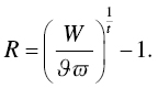
Adapted MPT has the investor declare ![]() , her maximum acceptable failure probability, so
, her maximum acceptable failure probability, so ![]() . The probability that our portfolio's return,
. The probability that our portfolio's return, ![]() , is less than our required return,
, is less than our required return, ![]() , must be less than or equal to
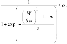
, must be less than or equal to ![]() . Using the logistic cumulative distribution function (for tractability), we can say that
. Using the logistic cumulative distribution function (for tractability), we can say that
Therefore, given our investor's declared failure probability, ![]() , we can say that
, we can say that
A rearrangement of this equation yields
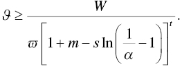
Since ![]() is the percentage of wealth allocated to the goal, adapted MPT carries an inherent contradiction when the investor's declared
is the percentage of wealth allocated to the goal, adapted MPT carries an inherent contradiction when the investor's declared ![]() mismatches what they have actually allocated to the goal!
mismatches what they have actually allocated to the goal!
This contradiction was deftly handled by Jean Brunel,16 who, rather than see it as a deficiency to overcome, used it as a tool. In essence, Brunel converted the inequality above to a strict equality and then used it as a way to allocate across goals. In other words, if an investor declares a maximum acceptable failure probability, Brunel uses the above relationship to convert the investor's declaration into an allocation to that goal. It is a solution to the problem of allocating wealth across goals. I admit, I was a bit starstruck by his cleverness! Unfortunately, though Brunel's solution does mostly solve the problem of across‐goal allocation within MPT, it does not get us all the way there. After the initial allocation across goals is done, our client is likely to either have wealth left over or—and this is more likely in my experience—not enough wealth to go around.17 What are we to do then? How do we rationally allocate any excess wealth, or rationally recall wealth from goals when there is not enough? We find ourselves back at square one.
A peer‐reviewer of the paper I published describing this problem questioned why this was even relevant. So what if we cannot allocate the exact amount of wealth in the wealth pool without client input and feedback? It is a fair question, especially in light of Brunel's solution. The answer is quite simple: Having an endogenous framework, a framework that does not require ongoing client input and feedback once the initial variables are ascertained, is critical to automating the solution and allowing for scale at the level of a wealth management firm. As will become extremely clear in later chapters, goals‐based solutions are hyper‐customized and hyper‐individualized. The only way to scale the delivery of those solutions, at the level of the firm, is to use the lever of technology. In short, everyday folks would never have access to the benefits of goals‐based solutions without a fully endogenous model, like the one I am presenting here. But more on that in later chapters.
The whole problem is further compounded by another basic assumption of MPT: unlimited leverage and short‐selling. Because investors are assumed to have no limit in their ability to borrow and sell short, MPT assumes there is no endpoint to the efficient frontier. However, all of us know that this is a silly assumption. Not only are investors constrained in their ability to borrow, but very often the mere costs of portfolio margin are prohibitive enough to eliminate any benefits. Shorting is outright prohibited in some account types. Not to mention, levering a client portfolio because MPT told us to is a sure way to have a regulator put you out of business! No matter how we slice it, there is an endpoint to the efficient frontier, and that presents a whole new set of problems.
When the investor's required return is less than the maximum return we can get on the efficient frontier, then goals‐based optimization is mathematically the same as mean‐variance optimization. If you agree with MPT and assume no endpoint to the mean‐variance efficient frontier, then this conversation is over—you can put this book down and move on to something more productive. However, when we do have an endpoint to the frontier, we find that, sometimes, an investor's required return is greater than the return offered by the efficient fronter. In that case, an investor maximizes the probability of achieving a goal by increasing variance, rather than minimizing it! This, of course, pushes portfolios off of the efficient frontier. Since I realize that this is economic blasphemy, allow me to demonstrate the point a bit more formally.
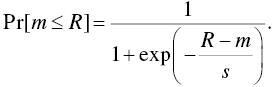
For tractability, let the probability of failure be defined by the logistic cumulative distribution function, so

where ![]() is the return required to achieve the goal,
is the return required to achieve the goal, ![]() is the expected return of the portfolio, and
is the expected return of the portfolio, and ![]() is the scale parameter (the logistic distribution's version of standard deviation). Let
is the scale parameter (the logistic distribution's version of standard deviation). Let ![]() , and we are concerned with the truthiness of
, and we are concerned with the truthiness of ![]() :
:
simplifying to
We are concerned with when ![]() , so
, so ![]() . Simplifying further yields
. Simplifying further yields
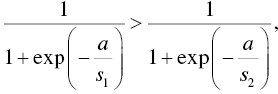
Recalling our original question of how the properties of ![]() affect the lowest probability of failure,
affect the lowest probability of failure, ![]() , it is now clear that the probability of failure is minimized when we choose the bigger
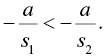
, it is now clear that the probability of failure is minimized when we choose the bigger ![]() ! We get the opposite conclusion when
! We get the opposite conclusion when ![]() , yielding
, yielding ![]() . Simplifying with that difference yields
. Simplifying with that difference yields
Hence, when the required return is less than the expected return, we minimize failure probability by minimizing variance—which is the mean‐variance paradigm. When our required return is greater than the expected return at the endpoint of the frontier, we minimize failure probability by increasing variance.
As the quadratic utility of MPT demonstrates, mean‐variance investors will never prefer a higher variance (because of the ![]() part) of the equation. Thus, adapted MPT has a whole class of portfolio solutions that are infeasible. That is, they return no result. More traditional MPT simply constrains‐away this problem by setting an additional optimization constraint that the portfolio's required return must be less than the endpoint of the efficient frontier.
part) of the equation. Thus, adapted MPT has a whole class of portfolio solutions that are infeasible. That is, they return no result. More traditional MPT simply constrains‐away this problem by setting an additional optimization constraint that the portfolio's required return must be less than the endpoint of the efficient frontier.
This simple demonstration shows that goals‐based portfolio optimization results in portfolios that are usually the same as mean‐variance optimized portfolios—that is, when ![]() . However, goals‐based portfolio optimization yields some portfolios that deliver a higher probability of achievement than mean‐variance optimized portfolios—that is, when
. However, goals‐based portfolio optimization yields some portfolios that deliver a higher probability of achievement than mean‐variance optimized portfolios—that is, when ![]() . Therefore, goals‐based portfolio optimization first‐order stochastically dominates mean‐variance optimization—a fancy way of saying that the results are the same, except in at least one case where the goals‐based approach yields a better result (see Figure 2.2). The traditional decision rules of economics demand we choose the stochastically dominant option.18 Furthermore, goals‐based portfolio optimization also yields results even when the results of adapted MPT are infeasible.
. Therefore, goals‐based portfolio optimization first‐order stochastically dominates mean‐variance optimization—a fancy way of saying that the results are the same, except in at least one case where the goals‐based approach yields a better result (see Figure 2.2). The traditional decision rules of economics demand we choose the stochastically dominant option.18 Furthermore, goals‐based portfolio optimization also yields results even when the results of adapted MPT are infeasible.
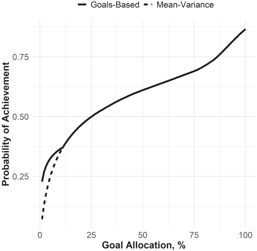
FIGURE 2.2 Stochastic Dominance of Goals‐Based Portfolio Optimization
When is an investor's required return greater than what is offered by the efficient frontier? Quite simply, it is when the goal is at the top of the Maslow‐Brunel pyramid. We colloquially call these goals dreams, aspirations, or even fantasies. Using the theoretical language we have put together, we can more technically say that these are goals that are not valued highly enough relative to other goals in the goals‐space to warrant a high enough allocation of the wealth pool to keep it on the efficient frontier.
That anyone is surprised such goals exist is a mystery to me. Obviously, we all have dreams and aspirational objectives. We all have goals we dream of achieving but would be just fine if we did not. We are willing to accept a much lower probability of achievement for these goals than we would for a goal lower on the pyramid, and, therefore, we allocate relatively few resources to them. More foundational goals, goals more central to our survival, carry more weight in our hierarchy, so they will naturally pull the majority of our resources. What is left over is usually dedicated to these less important, but more fulfilling, goals.
Before you simply accept what I am saying here, dear reader, let me say it a bit clearer. Sometimes it is rational to gamble! Yes, rational to gamble—sometimes. While theoretical blasphemy, this should be no surprise to any human operating in the real world. People gamble all the time, and not just with lottery tickets or roulette wheels. People gamble in markets by blindly buying options, or betting on a hot stock that otherwise makes no sense in a portfolio. What's more, people clearly do not gamble everything. People tend to gamble with a set amount of money and then let it go (barring a pathology, of course).
This behavior is predicted and recommended by the goals‐based framework! Where traditional utility theory yields people who are always and everywhere variance‐averse, goals‐based utility yields people who are variance‐averse with most of their wealth, but variance‐seeking with a little. Because people have multiple goals with varying degrees of importance, they will set a budget for the goals that require high variance to achieve. Again, this is exactly what we see in the real world.
Mathematics aside, allow me to justify the point with an extreme example. Imagine you owe a violent mafia loan shark $10,000 by the morning. Sadly, tonight, you have only $7,000. In desperation you walk into the economics department of your local university and approach the first professor you find. Explaining your situation, the economics professor follows the rational course: she administers a risk‐tolerance questionnaire and optimizes a portfolio using the mean‐variance method. “I'm sorry,” she reports, “there just isn't enough time for a 70% stock/30% bond portfolio to return 43% by tomorrow morning.” Do you leave, distraught, certain of your hospital visit tomorrow morning? No! The only rational answer is to go to a casino—how else would you avoid a hospital visit in the morning? You enter the casino and gamble until you have gained the required $3,000 or lost all of your bankroll.
To be fair, “go to a casino” is not entirely foreign to traditional utility theory. Traditional utility theory would expect some people to be variance‐seeking. The trouble is that, once proven variance‐affine, the “rational” course, according to traditional economics, is to gamble until all of your wealth is gone—there is no point of satiation. But that certainly isn't rational! No, in this extreme example, you would gamble until you had $10,000 (or $0), then you would leave the casino because you would have accomplished (or failed to accomplish) your goal.
In the final analysis, given all of the problems with using MPT in a goals‐based setting, it seems so much more sensible to adopt a framework that is designed for the intended setting. When the best theoretical map we have is tattered, hand‐corrected, and full of “beware of that,” “remember this,” and “thar be dragons,” we use what we have to get us where we are going. But no navigator keeps this map as primary when a more accurate one is available. Goals‐based portfolio theory is, at least in my view, a more accurate theoretical map. It yields feasible solutions when adapted MPT yields infeasible ones. Goals‐based optimization stochastically dominates MPT optimization when real world constraints are included (like limited short‐sells and limited leverage)—that is, it yields higher probabilities of goal achievement than MPT. Where traditional MPT has only a variance‐aversion parameter, goals‐based portfolio optimization accounts for all the variables that makes a goal a goal. Adapted MPT, though a better accounting of goals than traditional MPT, violates our axiom of attainment. And, the goals‐based framework provides a mechanism to allocate wealth both within and across goals, which is offered by neither traditional nor adapted MPT.
While MPT has served an important role in finance and economics, a role that goals‐based theory builds on, it is a less‐refined tool than goals‐based portfolio theory. This fact is evidenced by the myriad ad hoc heuristics designed to compensate for its flaws in the real world. People want to minimize the probability of failing to achieve goals, not minimize variance per se. People want to allocate to low‐value, low‐probability goals, and that requires leaving the efficient frontier in search of high‐variance, lottery‐like investments. People are constrained in their ability to borrow and sell short. It seems to me that investors and practitioners would both be better served by a model that is constructed with them and the real world in mind from the start, which is exactly how goals‐based portfolio theory has been built.
With the theoretical foundation now complete, let us address the practical questions of implementation. Because the foundation is different, the techniques will be somewhat unfamiliar. I will ask you to be patient as we explore these methods together, and I also humbly ask that you be open to finding your own, better, solutions. When you do, please share them! Research on this topic is an ongoing conversation, heavily informed by those of us who are in the trenches together.
Notes
- 1 O. Morgenstern and J. von Neumann, The Theory of Games and Economic Behavior (Princeton, NJ: Princeton University Press, 1944).
- 2 M. Allais, “Le comportement de l'homme rationnel devant le risque: critique des postulats et axiomes de l'école Américaine,” Econometrica 21, no. 4 (1953): 503–546.
- 3 H. Markowitz, Portfolio Selection: Efficient Diversification of Assets, vol. 16 (New York: John Wiley & Sons, 1959).
- 4 My instinct is that people do not weight probabilities objectively, though this would create problems for the existing framework of goals‐based portfolio theory. If I had to venture a hypothesis, I would suggest that people have an exponential weighting of probabilities, so that the move from a 90% to 95% probability of success is felt much more strongly than a 10% to 15% probability of success. I do not see why this should be necessarily irrational—why is it rational to feel a 5% probability move equally no matter where it is in the 0 to 1 spectrum? Of course, this is just a hypothesis. Some work is needed to prove it, one way or another.
- 5 J. Brunel, Goals‐Based Wealth Management (Hoboken, NJ: John Wiley and Sons, 2015).
- 6 A. Chhabra, “Beyond Markowitz: A Comprehensive Wealth Allocation Framework for Individual Investors,” Journal of Wealth Management 7, no. 4 (2005): 8–34, DOI:
https://doi.org/10.3905/jwm.2005.470606. - 7 H. Statman, “The Diversification Puzzle,” Financial Analysts Journal 60, no. 4 (2004): 44–53, DOI:
https://doi.org/10.2469/faj.v60.n4.2636. - 8 R. Deguest, L. Martellini, and V. Milhau, Goal‐Based Investing: Theory and Practice (World Scientific Publishing, 2021).
- 9 In their book, Modern Portfolio Theory and Investment Analysis, for example, Edwin Elton, Martin Gruber, Stephen Brown, and William Goetzmann (Hoboken, NJ: John Wiley & Sons, 2009) add the constraint that a portfolio's required return must be less than the maximal return offered by the efficient frontier.
- 10 That is not exactly true. In desperate times, it may well be rational to gamble everything; the model demonstrates this quite readily. However, I would expect that, for most practical applications, this is not the baseline case. Furthermore, and this is not a formal part of the model, goals are malleable and revokable, and goals tend to shift in response to both the opportunity set in the market as well as the resources available. Someone who loses 90% of their wealth is unlikely to maintain the same goals as before. More likely, this person's goals shift significantly (with considerable loss of utility), likely leading to a complete rewrite of their goals‐space. This is a deficiency of the goals‐based model as there is currently no way to account for the changing nature of individual goals. Goals, in this model, are simply taken as exogenous, and resources are reallocated when/if goals change, for whatever reason.
- 11 A negative value would indicate negative utility (disutility) of achieving the goal—this may well be appropriate in some contexts, as Brunel discusses the avoidance of “nightmares, fears, worries, and concerns.”
- 12 Markowitz, p. 242.
- 13 M. Guillemette and M. Finke, “Do Large Swings in Equity Values Change Risk Tolerance?” Journal of Financial Planning 27, no. 6 (2014): 44–50.
- 14 C. H. Pan and M. Statman, “Questionnaires of Risk Tolerance, Regret, Overconfidence, and Other Investor Propensities” Journal of Investment Consulting 13, no. 1 (2012): 54–63.
- 15 S. Das, H. Markowitz, J. Scheid, and M. Statman, “Portfolio Optimization with Mental Accounts,” Journal of Financial and Quantitative Analysis 45, no. 2 (2010): 311–334, DOI:
https://doi.org/10.1017/S0022109010000141. - 16 J. Brunel, Goals‐Based Wealth Management (Hoboken, NJ: John Wiley and Sons, 2015).
- 17 For example, suppose our investor has $1,450,000 to allocate across three goals. Using Brunel's method, we allocate $723,000 to goal A, $389,000 to goal B, and $124,000 to goal C. But that still leaves another $214,000 unallocated. How do we allocate that sum?
- 18 See, for example, J. Hadar and W. Russell, “Rules for Ordering Uncertain Prospects,” American Economic Review 59, no. 1 (1969): 25–34.