CHAPTER 13
As a Bridge Between Normative and Behavioral Finance
“We build too many walls and not enough bridges.”
—Isaac Newton
Of all the tools goals‐based portfolio theory adds to the practitioner's toolbox, I find myself most excited about what it may do for economic theory more broadly. Today, economic theory is split into two camps. There are the normative economists who focus on how we should behave. Then there are the behavioral economists who focus on how we actually behave. To date, each has a legitimate critique of the other. The normative economists acknowledge that people often violate rational rules of behavior, but they continue to insist that the rational course is the one prescribed by traditional theory. The behaviorists acknowledge that normative theory may well be rational, but it certainly isn't practical, nor is it often reasonable. Behavioral insights not only reveal how we actually behave, but they are a better predictor of the actions of people in the aggregate.
Goals‐based portfolio theory offers another lens through which we can view the apparent dichotomy of behavior and rationality. Indeed, I am convinced that people are not as irrational as we have so far believed. Rather, if we simply better understand their motivations, if we better understand what goals people are attempting to accomplish in the real world, then many of the normative‐behavioral paradoxes melt away. In this way, goals‐based portfolio theory offers a bridge between traditional normative theories of economics and more descriptive behavioral theories. Certainly, I should not be so bold as to assert that humans are always and everywhere rational. There are many real‐world situations where complete rationality is not only impractical, but entirely impossible.1 Even so, it is my objective in this chapter to illuminate just a few examples that may sketch an outline of this theoretical bridge. I should say: This chapter is directed toward theoreticians much more than practitioners. So, any readers who are uninterested can skip this chapter with no loss of narrative.
To illustrate how the goals‐based utility framework might help build this bridge, I have applied it to three classic normative‐behavioral utility paradoxes: the Friedman‐Savage puzzle, Samuleson's paradox, and the St. Petersburg paradox. I also include a discussion of the experiments that apparently show that individuals do not weight probabilities objectively—a central component of several behavioral theories. Finally, I show how a market composed of goals‐based investors might influence price discovery. Indeed, many pricing anomalies may not be anomalies at all—they may be the aggregate result of goals‐based investors behaving rationally.
GAMBLING, INSURANCE, AND THE FRIEDMAN‐SAVAGE PUZZLE
As a child, I remember my grandparents occasionally buying lottery tickets. They never spent significant money on them, of course, but buying a few tickets every week was a regular ritual for them. Since they owned two cars and a home, I feel it is safe to assume that they also purchased insurance. And, so, we have an example of our first paradox: real people who bought insurance and lottery tickets at the same time!
For most laymen, this does not seem a paradox at all. Of course people both gamble and take steps to protect their assets; this is common experience. Yet, normative economics does not allow for this. In normative theory, people are assumed to be everywhere averse to risk. Consider the following choice sets:
- 1A. $50 with certainty, or
- 1B. A coin flip: heads pays you $200, tails makes you pay $100.
Both of these offers carry the same expected value of $50, but the second one carries risk. It does seem silly to accept choice 1B when you could grab the $50 for sure—especially if you are playing this game over and over again, as investors do. Risk aversion simply means that you require more payoff than the certain outcome to prefer the risky to the certain choice. Something like:
- 2A. $50 with certainty, or
- 2B. A coin flip: heads pays you $300, tails makes you pay $100.
In this second choice, 2B offers $50 more than choice 2A in expected value. This is a risk premium. When playing the game repeatedly, and putting the law of large numbers on our side,2 we can harvest that extra return and come out further ahead than if we repeatedly chose 2A.
People are assumed to be risk averse in normative economics because it can be shown that people with risk‐loving attitudes will accept a negative risk premium for the risky choice. That is, they would accept less of a payoff than the certain outcome simply because it is the riskier choice. Something like:
- 3A. $50 with certainty, or
- 3B. A coin flip: heads pays you $150, tails makes you pay $100.
Here, 3B offers an expected payoff of $25 whereas 3A offers an expected payoff of $50. By choosing 3B, we are giving up an expected $25 per flip to choose the riskier outcome—that is a negative risk premium.
Normative theory does allow for an individual who prefers risk for its own sake. That is, there may well be people who would gamble because they enjoy gambling and are therefore willing to pay to do it. However, in normative theory, individuals are not expected to be both risk‐averse and risk‐loving at the same time. Why, then, did my grandparents buy both insurance and lottery tickets simultaneously? How could they be both risk‐averse and risk‐loving at the same time?
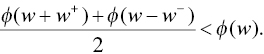
This is known as the Friedman‐Savage paradox, after the authors who were first to describe the problem.3 They also proposed a solution, suggesting that an individual's utility curve bends from concave (risk‐averse) to convex (risk‐seeking) along various points of wealth, and that there are points along that curve where people are willing to take risks with small amounts of wealth (such as a lottery ticket) and avoid risks with large amounts of wealth (such as a house).
Richard Thaler proposed another solution, one that is foundational to the goals‐based methodology. He suggested that people divide their wealth into mental “buckets” and that each bucket has a different risk tolerance. In some buckets, people are considerably more risk‐averse and in other buckets people may be risk‐seeking. Using our theoretical language, those buckets are simply goals, and some goals are valued highly enough to warrant less risk‐taking while others (higher on the Maslow‐Brunel pyramid) warrant more risk‐taking. This is no longer considered controversial and has almost become part of traditional theory.
Gambling, however, is still controversial. Nowhere in normative economics is gambling considered rational. People may do it, as described by behavioral models, but that is because people are irrational. Yet, goals‐based portfolio theory not only acknowledges gambling behavior but considers it rational in some circumstances, as we have already explored. I admit, this is tough for me to accept, but it is a plain fact of the math. If people seek to maximize the probability of achieving their goals, then there are circumstances when maximizing the volatility of outcomes is the optimal approach.
The Friedman‐Savage puzzle is a paradox in normative economics. And though it is predicted and described by behavioral economics, it is still considered irrational. In the goals‐based framework, however, it is not only predicted but is considered rational. Here is how the Friedman‐Savage puzzle is resolved under this paradigm.
First, we know that individuals have multiple goals. Rather than have one uniform variance‐aversion constant, goals‐based investors are assumed to have many different tolerances for risk—each informed by the objectives for a goal. However, in all cases, goals‐based investors want to maximize the probability of achieving their goals. Gambling, giving up return to maximize variance, is then rational when the return required to accomplish a goal is greater than the maximum return offered by the mean‐variance efficient frontier. This can be easily demonstrated more formally.
Let ![]() be the return required to attain our goal,
be the return required to attain our goal, ![]() is the portfolio return, and
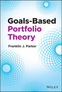
is the portfolio return, and ![]() is portfolio variance. We know that variance‐affinity is experienced when the second derivative of the utility function is positive, and variance‐aversion is experienced when the second derivative is negative (variance‐indifference is experienced when
is portfolio variance. We know that variance‐affinity is experienced when the second derivative of the utility function is positive, and variance‐aversion is experienced when the second derivative is negative (variance‐indifference is experienced when ![]() ). Using the logistic cumulative distribution function as our primary input of utility, we are concerned with
). Using the logistic cumulative distribution function as our primary input of utility, we are concerned with
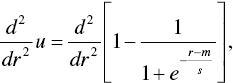
which is
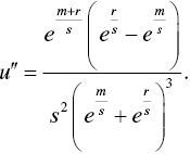
Since the bottom of the fraction is always positive,  , as is the coefficient in the numerator,
 ![]() , it must be so that
, it must be so that ![]() only when the term
only when the term ![]() is positive, meaning
is positive, meaning
must be true. Simplifying to isolate ![]() and
and ![]() :
:
leading to
Therefore, variance‐affinity is present when ![]() . By contrast,
. By contrast, ![]() only when
only when
yielding
leading to
Therefore, variance‐aversion is present when ![]() . This, of course, is a result echoing the one derived in Chapter 2.
. This, of course, is a result echoing the one derived in Chapter 2.
This is also confirmed by a simple inspection of the utility‐of‐wealth curve for goals‐based investors, shown in Figure 13.1. For lower values of wealth, the curve is clearly concave, while it is convex for higher values of wealth. Traditional utility theory tells us that concave utility curves are indicative of variance‐affinity and convex utility curves are indicative of variance‐aversion. Thus, goals‐based investors are variance‐averse for higher levels of wealth and variance‐affine for lower levels of wealth.
Counter to our training and intuition, the logic and subsequent math clearly demonstrates that, in some circumstances, gambling is entirely rational, and so is paying a small amount to protect a large amount. As it turns out, there is no paradox at all. People are, in fact, behaving rationally by buying both insurance and lottery tickets simultaneously.
Someone should tell my grandparents they were not so irrational after all.
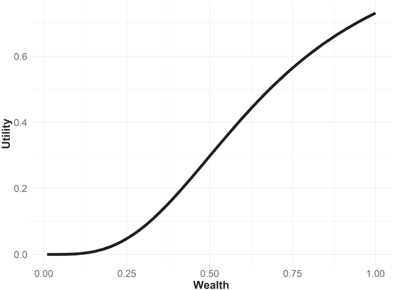
FIGURE 13.1 Goals‐Based Utility‐of‐Wealth Curve
Assuming 1.00 is needed in five years, and the portfolio returns 8% with 14% volatility.
SAMUELSON'S PARADOX
Famed economist Paul Samuelson—author of numerous economics textbooks, and winner of a Nobel Prize—once offered a colleague a bet:4 one coin flip, heads pays the colleague $200, tails the colleague pays $100. His colleague responded that he would not accept that bet but would accept a game of 100 such coin flips. Samuelson demonstrates how this is an irrational response in the context of normative utility theory. An individual who is not willing to lose $100 should not be willing to risk losing $100 one hundred times in a row, even though that may be a remote possibility. The paradox, then, is why Samuelson's intelligent and educated colleague would refuse an offer that should be taken and accept an offer that should not be taken.
Economist Matthew Rabin published a rebuttal of Samuelson's logic,5 showing that normative utility theory could not possibly be used to translate risk aversion from small stakes to large stakes. In short, Rabin showed that normative theories produced absurd results if we assume that risk tolerance scales up the wealth spectrum: “Suppose we knew a risk‐averse person turns down 50–50 lose $100/gain $105 bets for any lifetime wealth level less than $350,000… Then we know that from an initial wealth level of $340,000 the person will turn down a 50–50 bet of losing $4,000 and gaining $635,670.” Clearly an absurd result. Matthew Rabin and Richard Thaler press the point further6 invoking Monty Python's “Dead Parrot” sketch, going so far as to declare expected utility theory “a dead theory.”
What Rabin and Thaler do show is that risk‐tolerance is contextual, varying across the wealth spectrum, and that preferences for certain wealth levels cannot reflect preferences for other wealth levels. Of course, this is exactly what goals‐based theory predicts, but Rabin and Thaler press their point as a mark against the whole project of normative economics (Thaler, and to some degree Rabin, too, are both in the behavioral camp). That is ground, however, I am not yet ready to cede. Goals‐based portfolio theory may offer some relief here, showing that people may not be as irrational as normative theory would have us believe. Let us analyze Samuelson's offer through a goals‐based lens.
We can understand the colleague's utility before Samuelson's offer as
where ![]() is the value of the goal the colleague wishes to achieve,
is the value of the goal the colleague wishes to achieve, ![]() is the current wealth dedicated to the goal, and
is the current wealth dedicated to the goal, and ![]() is the probability of achievement function, given all the goal variables. For ease of discussion, I have removed the extra variables from our formulation. We can understand Samuelson's offer as
is the probability of achievement function, given all the goal variables. For ease of discussion, I have removed the extra variables from our formulation. We can understand Samuelson's offer as
where ![]() is the wealth gained if the colleague wins the coin flip, and
is the wealth gained if the colleague wins the coin flip, and ![]() is the wealth lost if the colleague loses the coin flip.
is the wealth lost if the colleague loses the coin flip.
The colleague did not accept the offer, so we can infer that ![]() , or
, or
and this simplifies to an interesting result:
In other words, if the amount of probability gained from a win is less than the probability that would be lost in a loss, the colleague should not take the offer. This can be easily seen by restating the above equation to
Recall that the goals‐based utility of wealth curve is convex for higher levels of wealth and concave for lower. We do not know where the colleague sits on that curve, of course, but there are places where the above inequality is satisfied. In other words, refusal of the offer may be entirely rational, depending on how much wealth the colleague has currently dedicated to the goal. To be fair, Samuelson never argues that it is irrational to turn down the offer. There is nothing revolutionary about this analysis so far.
Assuming 100 coin flips is a negligible increase in time, the colleague's counteroffer is an entirely different game. In fact, the probability of any loss7 whatsoever is 1/2300. Using these figures, let's analyze the colleague's counteroffer in a similar manner. Again, we are concerned with the truthiness of ![]() , or
, or
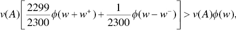
simplifying to
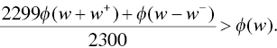
Given that the winning probability is weighted 2,299 times more than the losing probability, it would be quite a stretch to deny this offer, no matter how extreme the loss. Suppose, for the sake of discussion, that the offer was such that any loss would be catastrophic and result in a zero probability of success, so ![]() , then the problem simplifies to:
, then the problem simplifies to:
So long as the resultant probability given a win is greater than 1.004369 times the baseline probability, the colleague should accept the counteroffer. That is a move in probability of, say 62.000% to 62.271%. Rabin and Thaler are right to say, “A good lawyer could have you declared legally insane for turning down this gamble.”
Note, though, that the resolution of this paradox is not due to some behavioral flaw present in the colleague (and all of us). Rather, the paradox is an artifact of a flawed normative theory. When we look through the lens of goal achievement, the paradox ceases to exist. And, what's more, the colleague acted entirely rationally despite the claim of Samuelson and the intimation of Rabin and Thaler. In the end, whether the colleague should have accepted Samuelson's original offer is dependent on the value of variables that we do not know but rejecting it can be reasonably defended. In almost no circumstance should the colleague reject the counteroffer, however.
INFINITE PAYOFFS, LIMITED COSTS—THE ST. PETERSBURG PARADOX
In a previous chapter, we briefly discussed Daniel Bernoulli's critique of expected value theory. As a counterargument, Bernoulli proposed a gamble: An individual begins with an initial stake of $2 and we flip a coin. The initial $2 bankroll is doubled every time heads comes up, and when tails comes up the game is over and the winnings are the value of the bankroll. What is interesting about this game is that it has an infinite expected value:
where  is the probability of getting heads on the
 ![]() coin flip, and
coin flip, and ![]() is the payoff of that flip. The probability of winning the first flip is
is the payoff of that flip. The probability of winning the first flip is ![]() and the payoff is
and the payoff is ![]() . The probability of winning the second flip is
. The probability of winning the second flip is ![]() and the payoff is
and the payoff is ![]() . We can generalize the expected value of the gamble as
. We can generalize the expected value of the gamble as

And it becomes clear that the sum is infinity:
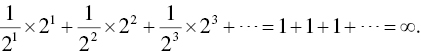
Since the game has an infinite expected value, Bernoulli argued that someone should be willing to pay any price to play the game! Obviously, no one would pay an infinite price to play this game, and therein lies the paradox.
The paradox can be solved if individuals do not weight probabilities objectively, as proposed by behavioral economics, but that solution implies that people are not behaving rationally when they pay a limited cost for the game. Since normative economics solves the paradox using the theory of marginal utility—that the utility of wealth grows slower than the raw payoffs, so the benefit reaches an apex—this is no longer considered a paradox. Even so, it is an interesting problem, and I find it a useful foil to further our intuition of goals‐based utility theory, hence my desire to include an analysis of the game here. With that, let's explore how goals‐based utility theory solves Bernoulli's paradox.
If our individual chooses to play the game, she stands to win ![]() with probability
with probability ![]() , and she stands to lose the cost of entry,
, and she stands to lose the cost of entry, ![]() , with probability
, with probability ![]() . We are trying to find the maximum cost an individual would incur to play the game, and that means that there is a cost at which the individual is indifferent to the gamble or the status quo. We can infer from that point of indifference the maximum cost she would be willing to incur to play the game. To find that point of indifference, we set her baseline probability of achievement equal to the probability of achievement if she plays the gamble:
. We are trying to find the maximum cost an individual would incur to play the game, and that means that there is a cost at which the individual is indifferent to the gamble or the status quo. We can infer from that point of indifference the maximum cost she would be willing to incur to play the game. To find that point of indifference, we set her baseline probability of achievement equal to the probability of achievement if she plays the gamble:
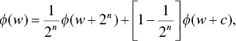
where ![]() is the probability of achieving her goal if the gamble is won and
is the probability of achieving her goal if the gamble is won and ![]() is the probability of achieving her goal if the gamble is lost and the cost of
is the probability of achieving her goal if the gamble is lost and the cost of ![]() is incurred.
is incurred.
Okay, we are forced to make some simplifying assumptions here. First and most obvious: no one can flip a coin an infinite number of times. Goals are time‐limited, so any real‐world analysis of the gamble must include the time it takes to flip coins and calculate winnings—not to mention how long humans are physically able to sit at the gambling table to participate in the game. Obviously, all of those answers are less than infinity, but by how much? Since the game itself is a thought‐experiment, and no casino offers the actual game, my purpose is not to provide a completely realistic analysis of the game. Rather, the purpose is to keep the spirit of Bernoulli's thought experiment and put our theory through its paces. In order to do that we have to assume that an infinite number of coin flips is at least possible to witness.
Second, we know that a goals‐based investor has a point of wealth satiation, so she will stop playing the game when ![]() , where
, where ![]() is the wealth required to fund her goal. This is helpful because it means we can solve for
is the wealth required to fund her goal. This is helpful because it means we can solve for ![]() , the number of flips our investor needs to accomplish her goal:
, the number of flips our investor needs to accomplish her goal:

By replacing ![]() with the ratio of the log of required wealth to the log of 2, we can keep the equation above limited to the goal‐variables and go about solving for the cost variable, but that also means that
with the ratio of the log of required wealth to the log of 2, we can keep the equation above limited to the goal‐variables and go about solving for the cost variable, but that also means that ![]() , the number of coin flips required to achieve the goal, may not be an integer. Obviously, we cannot flip a coin 6.64 times, but for the sake of this analysis we are going to assume that we can. Again, this is a thought experiment, not an actual gamble demanding exacting accuracy!
, the number of coin flips required to achieve the goal, may not be an integer. Obviously, we cannot flip a coin 6.64 times, but for the sake of this analysis we are going to assume that we can. Again, this is a thought experiment, not an actual gamble demanding exacting accuracy!
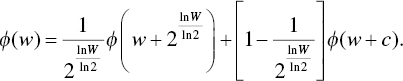
With these simplifying assumptions, we can press forward. Leaning on a logistic portfolio distribution (for tractability) we can set ![]() , replace
, replace ![]() and solve for
and solve for ![]() :
:
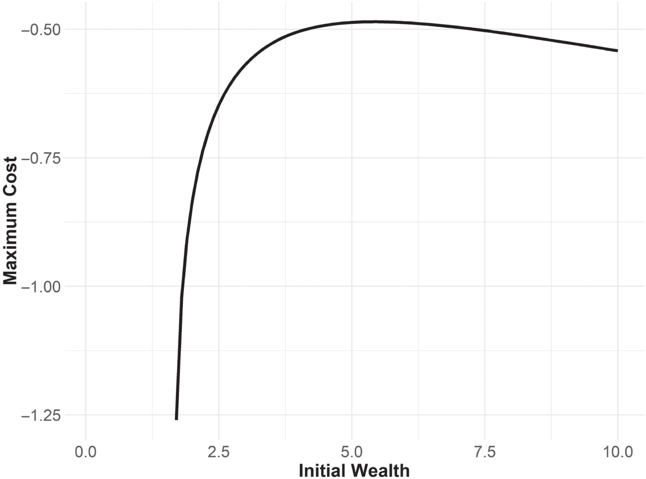
FIGURE 13.2 Willingness to Play the St. Petersburg Game
Where required wealth is 10, distributions are logistic, 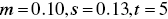 .
.
Reorganizing the equation to begin isolating the cost variable yields
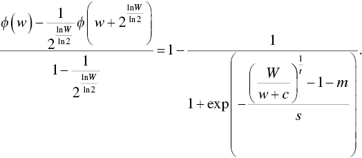
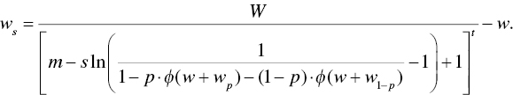
Applying some algebra leads to our general‐form cost function for a goals‐based investor playing the St. Petersburg game, shown in Figure 13.2:
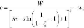
where
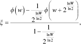
and
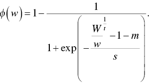
As has been the case in our goals‐based framework, how much an individual is willing to pay to play the St. Petersburg gamble is dependent, not just on the nature of the game, but also on her goal‐variables. I have plotted the individual's willingness to play the gamble given some example goal particulars. Interestingly, the results square with our intuition, at least mostly. When initial wealth is low enough, an individual is willing to spend all of her funds on the gamble, which is consistent with the ![]() portfolio structure we discussed in previous chapters. Gambling is rational for low‐probability goals. As initial wealth grows, willingness to pay drops very rapidly until peaking. After finding its peak, willingness again begins to increase as initial wealth increases, which is not what I would have expected. However, this is reflective of the portfolio's ability to recover the cost of the game through portfolio growth over time—the goal is overfunded, in other words, and some of that overfunding can be dedicated to a gamble, thereby increasing achievement probability.
portfolio structure we discussed in previous chapters. Gambling is rational for low‐probability goals. As initial wealth grows, willingness to pay drops very rapidly until peaking. After finding its peak, willingness again begins to increase as initial wealth increases, which is not what I would have expected. However, this is reflective of the portfolio's ability to recover the cost of the game through portfolio growth over time—the goal is overfunded, in other words, and some of that overfunding can be dedicated to a gamble, thereby increasing achievement probability.
What this analysis shows, quite clearly, is that a goals‐based investor would not pay an infinite amount to play the gamble, resolving the paradox. Behavioral economics has relied on subjective probability weights to solve the paradox, but that, of course, means that individuals are behaving irrationally with respect to the gamble. By contrast, the goals‐based solution is rational (assuming you accept the initial axioms). It would be very interesting to offer the gamble to real people in the real world (ideally for real money) and see if their behavior corresponds to the predictions of goals‐based utility theory. Unfortunately, I am not aware of empirical data on the subject, so this must be left for future research.
QUESTIONS OF PROBABILITY, QUESTIONS OF DOUBT
In 1953, as a critique of Von Neumann and Morgenstern's axiom of independence, economist Maurice Allais8 conducted an experiment. He offered his subjects two sets of choices:
| 1A: | $1,000,000 with 100% probability |
| 1B: | $1,000,000 with 89% probability |
| $5,000,000 with 10% probability | |
| $0 with 1% probability |
The second choice set:
| 2A: | $1,000,000 with 11% probability |
| $0 with 89% probability | |
| 2B: | $5,000,000 with 10% probability |
| $0 with 90% probability |
Allais found that people tended to choose choice 1A over 1B and also chose 2B over 2A. Though it is not immediately obvious, this is a contradiction!
From the first choice set we learn that ![]() , or
, or
which can be simplified to
In other words, we learn that an 11% chance of gaining $1,000,000 carries more utility than a 10% chance of gaining $5,000,000. We learn from the second choice set that ![]() , or
, or
which directly contradicts the first choice set!
Allais concluded that the axiom of independence cannot be a valid one because it fails to predict “reasonable people choosing between reasonable alternatives.” Markowitz rebutted that people choosing the wrong alternative acted irrationally, but that people are irrational does not negate the axiom. So the behavioral‐normative split was formed.
Later authors saw in Allais's results a clue: perhaps it is not the axiom of independence people do not intuit; maybe people do not weight probabilities objectively. Allais's paradox can be solved if people feel the move from 99% to 100% more than they feel the move from 10% to 11%. This idea led to numerous papers in behavioral finance, all of them offering a theory as to why people choose seemingly contradictory choices. It was Daniel Kahneman and Amos Tversky's cumulative prospect theory, however, that seems to have been accepted as the answer. Cumulative prospect theory has two basic components. The first component deals with how people value gains in wealth versus losses in wealth. The second component is that people do not weigh probabilities objectively, but rather tend to overweight low probability events and underweight high probability events, as Figure 13.3 demonstrates. This result has been confirmed in experiments by other researchers and is now widely accepted as true.
While I do not suggest that people objectively perceive probabilities always and everywhere, it is worth noting that the method used by researchers to derive these results may be tainted if individuals are processing the experiment through a goals‐based lens. To fully understand why, we need to look more closely at the experiment.
When testing for subjective probability weights, it is standard practice to determine the certainty equivalent of an offer. The certainty equivalent is derived by offering the subject a gamble, then finding the certain amount of money that makes her indifferent to the gamble or the sure outcome. For example, suppose I flip a coin. If it lands heads, I pay you $100, if tails you get $0. Now I offer you a choice between that gamble and a sure amount of money. What amount of certain money makes it so that you are indifferent to the gamble of the certain outcome? That amount of money is your certainty equivalent.
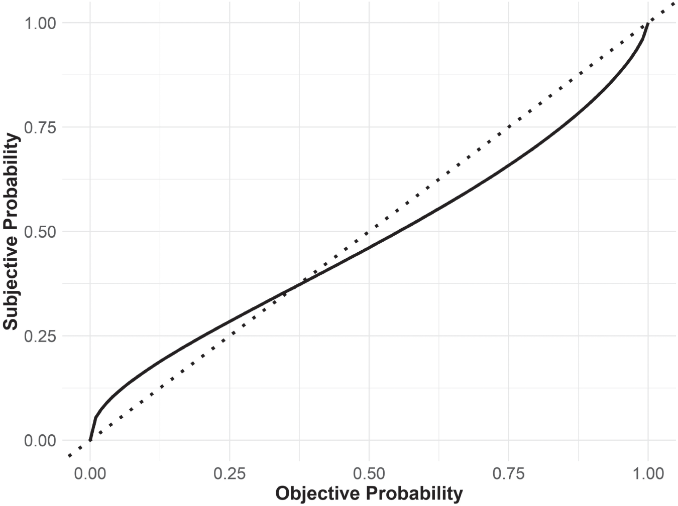
FIGURE 13.3 Standard Probability Weighting Function9
Here is the key to the goals‐based critique: to derive how the subject is perceiving the probability of the gamble, we divide the certainty equivalent by the expected wealth offered in the gamble. That ratio is interpreted as the probability that is perceived by the subject. Continuing our coin flip example, suppose you were indifferent to $40 for sure or the $100 for heads/$0 for tails gamble. We would then infer that you perceive the 50% probability of the coin flip as ![]() —an underweight of 10% points. However, when we look at this experiment through a goals‐based lens, we can make a case that the results may not indicate what they have been so far interpreted to indicate. Let's dive into why.
—an underweight of 10% points. However, when we look at this experiment through a goals‐based lens, we can make a case that the results may not indicate what they have been so far interpreted to indicate. Let's dive into why.
We can understand the certainty equivalent as the point where the utility of the gamble equals the utility of the sure thing, or ![]() . Let's set up this equality with a bit more detail:
. Let's set up this equality with a bit more detail:
Note that ![]() is the initial wealth dedicated to the given goal,
is the initial wealth dedicated to the given goal, ![]() is the sure amount of wealth on offer,
is the sure amount of wealth on offer, ![]() is the amount of wealth if the gamble is won,
is the amount of wealth if the gamble is won, ![]() is the amount of wealth if the gamble is lost,
is the amount of wealth if the gamble is lost, ![]() is the probability of winning the gamble,
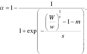
is the probability of winning the gamble, ![]() is the probability of achieving the needed return given the inputs (it is an upper‐tail cdf), and that people will evaluate wealth offers within the context of goal achievement, of which this wealth will be an input. As mentioned above, the certainty equivalent is the ratio of sure wealth divided by the gamble wealth, or
is the probability of achieving the needed return given the inputs (it is an upper‐tail cdf), and that people will evaluate wealth offers within the context of goal achievement, of which this wealth will be an input. As mentioned above, the certainty equivalent is the ratio of sure wealth divided by the gamble wealth, or ![]() , using the symbology in our equation. Because
, using the symbology in our equation. Because ![]() is typically given, and we assume
is typically given, and we assume ![]() is logistic, then we can use a little algebra to rearrange the above equation to find
is logistic, then we can use a little algebra to rearrange the above equation to find ![]() , given the other inputs. We find:
, given the other inputs. We find:
From here we can play with the inputs to estimate how a goals‐based investor might react to the experiment. The results are rather intriguing. The plot shows two types of goals, one aspirational and the other a standard goal. Recall that our technical definition of an aspirational goal is one where the return required to hit the goal is greater than the return offered by the last portfolio on the efficient frontier (or in this case, it is simply greater than the portfolio return assumption). A foundational goal is one in which the return required to attain the goal is less than the maximum portfolio return.
For aspirational goals, we find that the goals‐based utility model accurately predicts how individuals will behave in this experiment. The ratio of the certain offer to the gamble offer mirrors the standard probability weighting function from the literature (and may help explain the wide range of results experimenters have logged).10 For foundational goals, the model shown in Figure 13.4 returns an interesting result! For foundational goals, individuals will behave in a way almost consistent with what normative economics would predict. That is, the amount of certain wealth that makes the individual indifferent to that offer or the gamble will be about equal to the probability of winning the gamble. So, for example, if we offer a goals‐based investor a 30% probability of winning $1, we will have to offer a certain $0.29 to make her indifferent to the choices. Normative economics would expect that we would have to offer a certain $0.30—not too different a result.
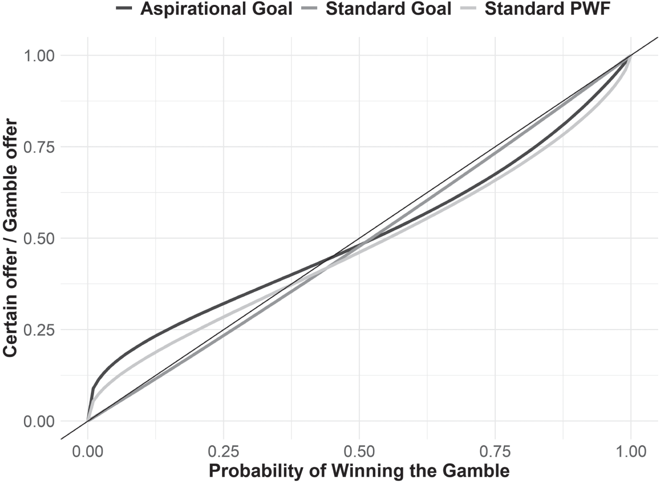
FIGURE 13.4 Goals‐Based Utility Prediction of Probability Weighting Experiments and Comparison to Standard Probability Weighting Function
Again, the point here is not to argue that individuals are weighting probabilities objectively.11 Rather, this demonstrates the robustness of the goals‐based utility model, but, more importantly, calls into question the behavioral‐normative divide in economics. Remember, if we accept the axioms of goals‐based utility theory as rational, then behavior that is consistent with the model is rational. Individuals may not behave as irrationally as we have previously believed! For offers with small money stakes among individuals with few long‐term financial goals (like college students on whom many of these experiments were conducted, for example), these experiments validate how goals‐based investors react to gambles when aspirational goals are at stake. When individuals have real money and real goals on the line we can expect that they will behave much differently, and that behavior is much more in‐line with what normative economics would expect.
On the downside, half of Tversky and Kahneman's cumulative prospect theory is a probability weighting function. If we call that component into question, it does lead to questions about the theory as a whole—a theory cited by over 17,000 papers and which earned Daniel Kahneman a Nobel Prize in Economics. I would not be so bold to assert that these conclusions topple so widely accepted a theory. Yet, at a minimum, it seems to call for further exploration by researchers.
Yet again, goals‐based utility theory may offer a bridge between normative and behavioral economics—a bridge that is being built by others, as well. There is a certain wisdom in the crowd, as we all know, and I have found that people generally operate in their own best interest, even if that is via intuition and nonquantitative methods.
IRRATIONAL PEOPLE, IRRATIONAL MARKETS?
As goals‐based investors aggregate, it seems clear that they will have an effect on market pricing. People are not isolated and, hard as it may be to remember these days, markets are comprised of real people. If these people were entering markets not for the fun of it but because they had specific objectives, that would carry some interesting consequences for the pricing mechanism. In this section, I would like to explore some interesting outcomes of market pricing if people are behaving in ways consistent with goals‐based utility theory.
As we have explored, investors will seek to maximize the probability of attaining a goal. However, when considering something like pricing dynamics, it may be easier to simply analyze a line of indifference—that is, the points at which utility stays the same if we vary the other inputs. We assume that investors enter capital markets attempting to get a probability of goal achievement of at least ![]() , but greater than
, but greater than ![]() is obviously preferred. This treats the probability of goal achievement as a risk‐aversion metric, which is essentially what it is. So, we can set up our form like this:
is obviously preferred. This treats the probability of goal achievement as a risk‐aversion metric, which is essentially what it is. So, we can set up our form like this:
where ![]() is the minimum probability our investor is willing to accept to achieve the goal,
is the minimum probability our investor is willing to accept to achieve the goal, ![]() is the initial amount of wealth dedicated to the goal,
is the initial amount of wealth dedicated to the goal, ![]() is the amount of wealth required to achieve the goal, and
is the amount of wealth required to achieve the goal, and ![]() is the time horizon within which the goal must be accomplished. Using the logistic cumulative distribution function, our equation becomes
is the time horizon within which the goal must be accomplished. Using the logistic cumulative distribution function, our equation becomes
From here, we can solve for ![]() , or the minimum acceptable return, given some acceptable level of
, or the minimum acceptable return, given some acceptable level of ![]() :
:
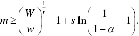
In other words, an investor will enter capital markets attempting to get at least ![]() , but willing to take more
, but willing to take more ![]() if it is offered. Naturally, this minimum acceptable return is driven by all of the goal variables relevant to the investor—how much money she has dedicated to the goal, how long until the goal is to be funded, how volatile the asset is, and the minimum acceptable probability of achievement.
if it is offered. Naturally, this minimum acceptable return is driven by all of the goal variables relevant to the investor—how much money she has dedicated to the goal, how long until the goal is to be funded, how volatile the asset is, and the minimum acceptable probability of achievement.
With this rough model in mind, consider Figure 13.5 as representative of a very simple market, where we have three potential investors, A, B, and C. Each has different inputs to their minimum acceptable return equation, hence, as the expected volatility of the asset moves higher (on the horizontal axis), we find that each investor has a shifting minimum level of return—again, this is to maintain their minimum acceptable probability of goal achievement, ![]() . To illustrate the point, let us further suppose that all investors agree on the fundamentals of the security: that it will deliver volatility of
. To illustrate the point, let us further suppose that all investors agree on the fundamentals of the security: that it will deliver volatility of ![]() in the future. What we find is that investor A requires the highest return to invest in this security, represented by
in the future. What we find is that investor A requires the highest return to invest in this security, represented by ![]() . Investor C requires the second‐highest return,
. Investor C requires the second‐highest return, ![]() , and investor B requires the lowest return,
, and investor B requires the lowest return, ![]() .
.
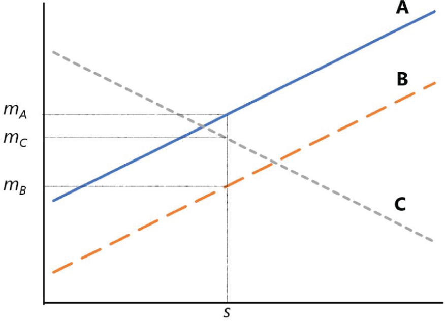
FIGURE 13.5 A Simple “Market” of Goals‐Based Investors
Pressing this a step further. If we think of price as some function of this minimum acceptable return, perhaps most simply as its inverse, ![]() , then we can conclude that even though every investor in the market may agree on the fundamentals of a security, they are each willing to pay an entirely different price!
, then we can conclude that even though every investor in the market may agree on the fundamentals of a security, they are each willing to pay an entirely different price!
Take the difference between investor A and investor B. Both require a minimum 65% chance of success, and they both need $1 in 10 years. However, investor B has more current wealth than investor A ($0.75 vs. $0.55). This one change means that investor B is willing to pay a higher price (accept a lower return) than investor A for the same security. Again, it is not that A and B disagree on the behavior of the investment—they both agree that it will carry volatility of ![]() . Rather, they simply have different needs, and this leads to disparate pricing.
. Rather, they simply have different needs, and this leads to disparate pricing.
Investor C is, of course, an oddity. C is willing to accept lower returns for higher volatility, counter to traditional theories of risk. Investor C, however, is acting perfectly rationally for an aspirational investor, as we have discussed. Investor C has a mere $0.22 dedicated to a $1.00 goal needed in 12 years (a required return of 13.4%). Because investor C has a minimum probability of achievement of 35%, this leads to a willingness to accept lower returns for higher volatility (of course, she would be willing to accept a higher return, were it offered).
If, then, all investors agreed that this portfolio were to yield ![]() volatility in the coming period, we should find that investor B will pay the highest price for it. Investors A and C will sell to B until B's liquidity is exhausted. Recall from above that investor B has $0.75 of liquidity dedicated to the goal, which is more than either investor A or investor C individually, but it is not more than A and C taken together. Even so, we should expect investor B to dominate the pricing in our simple market since she has the most liquidity. Once B's liquidity is exhausted, we would see the investment's price drop to the price investor C is willing to pay, and investor A will sell to investor C until investor A has no inventory (or C's liquidity is exhausted).
volatility in the coming period, we should find that investor B will pay the highest price for it. Investors A and C will sell to B until B's liquidity is exhausted. Recall from above that investor B has $0.75 of liquidity dedicated to the goal, which is more than either investor A or investor C individually, but it is not more than A and C taken together. Even so, we should expect investor B to dominate the pricing in our simple market since she has the most liquidity. Once B's liquidity is exhausted, we would see the investment's price drop to the price investor C is willing to pay, and investor A will sell to investor C until investor A has no inventory (or C's liquidity is exhausted).
An interesting wrinkle: why would any investor sell in this simple market? If A sells to B, for example, that would leave A with no investment at all, and with a lower probability of goal achievement than if she held some investment. It is here that the simplicity of the illustration breaks down. In truth, every investor would be running this process for every investment in the marketplace and selling one investment very likely means purchasing another with that new liquidity. What's more, almost never will investors exactly agree on the fundamentals of a security, so not only are investors bidding their needs in to the price, but also their view of the fundamentals. In other words, if there is no alternative to the existing investment, then the existing investment will not be sold unless the price is even higher—a dynamic market veterans know all too well.
My ultimate point here is not to build a complete and accurate model of market pricing dynamics. Rather, my point here is that markets price more than just security fundamentals, they price investor needs, too. For example, if you give investors more cash today, they become willing to pay a higher price for the exact same fundamentals. This could be why the global coordinated quantitative easing program seen through 2020 and 2021 has lifted the valuation metrics of markets (expanded P/E ratios, for example). Investments may be overpriced from an historical fundamentals perspective, but not necessarily from a liquidity perspective. By printing cash and pushing it into the hands of investors, prices rose even without a shift in business fundamentals—much to the consternation of value investors. Of course, we should expect the opposite to be true. As excess cash gets drained from the pockets of investors, they become less willing to pay higher prices and—all else equal—valuation metrics should shrink.
It cannot be enough, then, to simply analyze the fundamentals of a given security or portfolio. The marketplace of that security's investors must also be considered. Though we cannot expect to know every goals‐based variable for every investor, we should be able to make some broad‐brush assumptions. We should expect to find some securities dominated by aspirational‐type investors, variance‐seeking and likely quite active. For other securities, we should find an investment marketplace dominated by long‐term, variance‐averse investors who are seeking steady returns given their already‐stable financial positions. In both cases, we could do well to model the effects of changing security fundamentals, as well as changing investor variables, at least to the extent we can estimate them.
In his book Fractal Market Analysis, Edgar Peters comes to a very similar model of the marketplace:
Take a typical day trader who has in investment horizon of five minutes and is currently long in the market. The average five‐minute price change in 1992 was –0.000284%, with a standard deviation of 0.05976%. If, for technical reasons, a six standard deviation drop occurred for a five‐minute horizon, or 0.359 percent, our day trader could be wiped out if the fall continued. However, an institutional trader—a pension fund for example—with a weekly trading horizon, would probably consider that drop a buying opportunity because weekly returns over the past ten years have averaged 0.22 percent with a standard deviation of 2.37 percent. In addition, the technical drop has not changed the outlook of the weekly trader, who looks at either longer technical or fundamental information. Thus, the day trader's six‐sigma event is a 0.15‐sigma event to the weekly trader, or no big deal. The weekly trader steps in, buys, and creates liquidity… .
Thus, the source of liquidity is investors with different investment horizons, different information sets, and consequently, different concepts of “fair price.”12
It is this last point that I have attempted to demonstrate in this section. Every investor has a different “fair price.” In fact, an investor may not even agree with herself on “fair price” across her accounts. For one goal, x may well be fair, but for another goal x may be far too low a price!
Peters makes another profound and important point:
If all information had the same impact on all investors, there would be no liquidity. When they received information, all investors would be executing the same trade, trying to get the same price.
It is because fair price is dependent on so many individual variables that we see the volume of shares traded that we do! If fair price were readily agreed on in perfectly rational markets, trading would cease and markets would not be so liquid.
Indeed, the marketplace of goals‐based investors looks very fractal, supporting many of Peters's arguments. Within the marketplace, you have tens of thousands of individual security markets. These security markets have groups of individuals, each with similar characteristics, pushing this way and that (think of retired individuals who are trading with those nearing retirement, those who are in their early 40s, and those who just started saving). Each demography has its own general fair price, based on their shared variables. But within each demographic group, you also have sub demographics, and still further subdivisions of those groups. Each of those subgroups has its own approximation of fair price. Finally, we have the individual, who is herself divided with respect to pricing across each account, as each goal will have a separate fair price for a security. All of that sounds quite fractal to me.
Goals‐based portfolio theory, then, may better explain some pricing anomalies, as well as offer market practitioners some insight on how large‐scale forces might influence prices in the aggregate. While it is beyond the scope of this discussion, goals‐based portfolio theory may yield interesting fruit in not just macroeconomic theory, but also market microstructure theory. There is plenty of work yet to be done.
Notes
- 1 Satisficing models fall into this category, for example. Since people cannot know everything, decisions will necessarily be based on limited information. Individuals, then, get “enough” information to make a reasonably informed decision, even if it may not be the exactly optimal one if all information were known. See, for instance, D. Navarro‐Martinez, G. Loomes, A. Isoni, D. Butler, and L. Alaoui, “Bounded Rational Expected Utility Theory,” Journal of Risk and Uncertainty 57, no. 3 (2018): 199–223. DOI:
https://doi.org/10.1007/s11166‐018‐9293‐3. - 2 The law of large numbers is a very controversial topic in both goals‐based utility theory and traditional economics. Understanding when it does and does not apply is of prime importance. This is a point Vineer Bhansali makes in his book Tail Risk Hedging: Creating Robust Portfolios for Volatile Markets: “We really get one chance to save for retirement… The reality is that markets take one path, so the law of large numbers is no insurance against market crisis.” More broadly, this has become known as the ergodicity problem. For an insightful treatment, see O. Peters, “The Ergodicity Problem in Economics,” Nature Physics 15 (Dec 2019): 1216–1221. DOI:
https://doi.org/10.1038/s41567-019-0732-0. - 3 M. Friedman and L.J. Savage, “The Utility Analysis of Choices Involving Risk,” Journal of Political Economy 56, no. 4 (August 1948): 279–304.
- 4 Whether the offer actually happened or whether it was a foil to launch a discussion is not really known. In either case, the point stands. The more nuanced result Samuelson reached was that the risk‐aversion that can be calculated from the refusal of a small‐stakes offer would indicate risk‐aversion for large‐stakes offers, and also refusal of the colleague's counteroffer. Cf. P. Samuelson, “Risk and Uncertainty: A Fallacy of Large Numbers,” Scientia 98 (1963): 108–113.
- 5 M. Rabin, “Risk Aversion and Expected Utility Theory: A Calibration Theorem,” Econometrica 68, no. 5 (2000): 1281–1292.
- 6 M. Rabin and R. Thaler, “Anomolies: Risk Aversion,” Journal of Economic Perspectives 15, no. 1 (2001): 219–232.
- 7 We learn this from Rabin and Thaler (2001), who ran the numbers. I won't repeat their work here.
- 8 M. Allais, “Le Comportement de l'Homme Rationnel devant le Risque: Critique des Postulats et Axiomes de l'Ecole Americaine,” Econometrica 21, no. 4 (1953): 503–546.
- 9 From: D. Prelec, “The Probability Weighting Function,” Econometrica 66 (1998): 497–527. Prelec's probability weighting function is
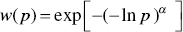 , with
  . In the case of this illustration,
  .
. - 10 See, for example, A. Tversky and D. Kahneman, “Advances in Prospect Theory: Cumulative Representation of Uncertainty,” Journal of Risk and Uncertainty 5, no. 4 (1992): 297–323.
Also R. Gonzales and G. Wu, “On the Shape of the Probability Weighting Function,” Cognitive Psychology 38, no. 1 (1999): 129–166.
- 11 Much to my chagrin, Allais's paradox cannot be solved, even in a goals‐based paradigm, unless investors weigh probabilities subjectively. This, of course, has implications for the rest of our goals‐based framework, but all of that is beyond the scope of this discussion. Again, it is a wonderful topic for future research!
- 12 Edgar Peters, Fractal Market Analysis: Applying Chaos Theory to Investment and Economics (New York: John Wiley & Sons, 1994), 42–43.