CHAPTER 5
Measuring the Return on a Real Estate Investment
Ever since Neanderthal Man first sublet the summer cave, income-property owners have been devising methods of measuring the success of their investments. In this chapter, we’re going to look at several of these methods and discuss their usefulness to modern-day investors. We’ll start with some of the cash flow measurements that have their origins in the precomputer days and work our way along to the more sophisticated techniques, such as internal rate of return.
Payback Period, Cash-on-Cash Return, Gross Rent Multiplier, Debt Coverage Ratio
One of the oldest and simplest measures is the payback period. You can define this as the length of time required to recover your initial cash investment. Let’s say you invest $100,000 in cash to purchase a $500,000 property. The balance, of course, is financed. The property generates a positive cash flow of $20,000 per year. Hence, the payback period is five years. To achieve a quick payback, your property must have a strong positive cash flow. The sooner you get your investment back, the sooner you can begin to “make” money. Sooner is better.
The payback period has been known colloquially as the “bingo year,” presumably because that is what the savvy and sophisticated investor would exclaim upon seeing the return of the Prodigal Down Payment. In the preceding example, the investor would have described year 5 as his or her bingo year.
One weakness of this method is that it does not take into account the time value of money. It treats a dollar received at some future date as being just as valuable as a dollar received—or invested—today. Looking again at the preceding example, if the property had no cash flow at all for four years and then $100,000 in year 5, it would still represent a five-year payback. However, you would have missed the chance to collect and reinvest $20,000 per year for the first four years. Even if you had reinvested the early cash flows at money market rates, you would certainly have accumulated some interest by the end of year 5. One five-year payback of $100,000 is not necessarily as good as another.
A method that is similar to the payback period is the cash-on-cash return. With this approach, you look at the cash flow (usually before taxes) from a particular year of a property’s operation—customarily the first year—and compare it with the cash you invested to purchase that property. You express the result as a percentage, so if you have a $10,000 cash flow this year from a property in which you initially invested $100,000 of your own cash, you would have a 10% cash-on-cash return.
Cash-on-Cash Return = Cash Flow before Taxes / Cash Investment
Cash-on-Cash Return = 10,000 / 100,000
Cash-on-Cash Return = 10%
The cash-on-cash return is perhaps even less illuminating than the payback period because it considers a property’s performance over just a single year. Nonetheless, it has typically been a very popular measure, probably because it expresses its result as a simple rate of return. It is easy to look at such a number and say, “A rate of 10% is better than the rate I can get on a T-bill. I like that.”
Both the payback period and the cash-on-cash return are entirely dependent on the property’s cash flow, which is just one of the four ways you can make money with a real estate investment, as discussed in our Introduction. As such, these measurements can obscure the truth as easily as they can reveal it. On the face of it, cash flow is good. One way to enhance a property’s cash flow for a particular year, however, might be to spend little or no money on maintaining that property. Deferring maintenance or improvements can prop up a sagging cash flow, at least for the short term, and give the appearance of a higher cash-on-cash return. The very actions that might increase the apparent return would, at the same time, make the property less attractive and ultimately less valuable.
Consider next a situation that is quite the opposite. Suppose that you can substantially increase a property’s value in the long run, but at the expense of its cash flow in the short run. Examples should come to mind easily. A five-year program of repairs and capital improvements might decimate your cash flow, but it might also ultimately attract better tenants and produce a more robust income stream. In so doing, you increase the value of the property so that the real profit can be realized at a later time, perhaps when you sell.
The point here is obviously not to say that a strong cash flow is bad and a weak cash flow is good. You need to recognize that cash flow–based measures of investment quality look at only a part of the total investment picture. They can lead you astray if you don’t take the time to look behind the numbers.
A cousin to the cash flow measures is the gross rent multiplier (GRM). GRM is a method of estimating or expressing a property’s value as a multiple of its gross rental income.
Gross Rent Multiplier = Market Value / Gross Scheduled Income (annual)
By transposing this equation, we also get:
Market Value = Gross Rent Multiplier × Gross Scheduled Income (annual)
There is probably no more basic way to evaluate an income property, and yet this technique still has some usefulness. Most of us are familiar with the “comparable sales” approach that is used to estimate the value of a home. If your neighbors’ homes are similar to yours in size and finish, and if several sold recently for $300,000 to $325,000, then yours should sell for a price in that same range. The GRM is a technique that looks at comparable income-producing properties and establishes a typical income multiplier. If other properties have sold recently for seven times gross income, then the subject property should also be worth about seven times its gross income.
This approach achieved its ascendancy in the precomputer (indeed, the precalculator) days for obvious reasons. As a potential buyer, you could stand on the sidewalk, gaze appreciatively at the property, multiply the rent by some whole number without even moving your lips, and determine immediately if the seller were anywhere close to serious.
This simplicity notwithstanding, GRM can be useful. It does overcome some of the hazards of the cash flow methods by making a partial end run around the operating expenses and capital improvement costs of the subject property. By using comparable sales and establishing a rent multiplier based on a number of other properties, GRM essentially establishes by default a typical level of annual expenses and improvements for this group of properties. If the subject property belongs in the group (i.e., if it is comparable to the others), then it should have comparable expenses. Hence, a seller could not distort your estimate of value by temporarily deferring maintenance. You might still undervalue a property, however, if its gross rent had not yet caught up to the seller’s ambitious rehabilitation of the property.
An investment measure that remains widely used is the debt coverage ratio, aka debt service coverage ratio. This is the ratio between the annual net operating income and the annual debt service.
Debt Coverage Ratio = Net Operating Income / Annual Debt Service
A property with a 1.20 debt coverage ratio has income before debt service that is 1.20 times as much as the debt service—in other words, the property generates 20% more net income than it needs to make its mortgage payments.
All the measures discussed here have at least the potential for shedding some light on the quality of our real estate investment, especially if we are comparing properties. None, however, succeeds in encompassing the whole investment, from acquisition to disposition. You need to consider not just the gross revenue and cash flows, but the timing of those income streams; and you certainly need to look at how the resale of your property will impact the overall success of your investment.
The proliferation of personal computers and of powerful software now makes it possible to create much more refined analyses that do indeed take into account issues such as resale and cash flow timing. You can even project varying holding periods, financing terms, and revenue streams, and you can test their impact on the overall success of your income-property investment. Let’s look at some more powerful analytical measures, such as capitalization rate and discounted cash flow.
Capitalization Rate
We’ve already discussed “capitalization rate,” or “cap rate,” as it is usually called. To review, we define cap rate as the ratio between a property’s net operating income (NOI) and its value.
Capitalization Rate = NOI / Value
You recall that a property’s NOI is its gross scheduled income, less vacancy and credit loss, and less operating expenses.
less Vacancy & Credit Loss
less Operating Expenses
= Net Operating Income
Operating expenses include insurance, utilities, maintenance, and similar items, but they do not include mortgage payments, depreciation, capital expenditures, or income taxes. Hence, the NOI is the net income before debt service, capital costs, and income taxes.
Like GRM, cap rate is not a cash flow measure. You could mortgage the property up to the ridge beam and wipe out any hope of a positive cash flow. That malfeasance would have no effect at all on the property’s NOI and hence none on its cap rate. Unlike GRM, how-ever, cap rate is not strictly based on revenue. It is based rather on net operating income—that is, revenue after the deduction of operating expenses.
The benefit of using capitalization rate as a measure of a property’s performance lies in part in the fact that nearly everyone else does. It is perhaps the easiest to calculate of the useful measures and is a good tool to compare a property’s current performance with that of similar properties. Other investors, lenders, and brokers are probably going to know just what you mean when you say that a property “has a 12% cap.” Since its use is widespread, data about prevailing cap rates are also readily available. Appraisers, brokers, and independent services can provide you with the typical cap rate for a particular type of property in a given location. The availability of that information can help you in determining if the property you are evaluating is an underachiever or overachiever compared with the market.
The downside to the capitalization rate, however, is the same as with most of the others we’ve considered so far. It looks at the property at a point in time (usually the current year) without regard to the property’s expected performance over your entire holding period. It can certainly be useful to look at a single point in time—what’s a reasonable estimate of value of the property today, and what is it likely to be worth in 10 years? But surely that doesn’t give you a sense of the performance of the property over time. Investors buy the whole timeline. They commit a certain amount of cash to purchase the property on day 1, and they expect to receive periodic cash flows thereafter, including the proceeds of an ultimate resale.
Derived Capitalization Rate
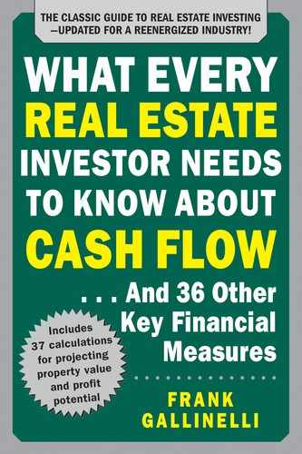
It would not be unreasonable to ask, “Where do cap rates come from?” If the stork doesn’t bring them, who does? The cap rate we have been talking about thus far is the rate that prevails in your particular marketplace; hence it is usually called the “market cap rate.” You can dissect that rate, however, using an approach called “band of investment” or “derived cap rate.” The derived cap rate breaks the calculation of the return into two components: financing and equity. The lender is getting a return on the financing; the investor is getting a return on the equity; the derived cap rate is the weighted average of the two.
A simple example should illustrate the process. Examine this calculation:
You are purchasing a property with 20% equity and 80% financing. You find that loans are available for 15 years at 7%. You start with the financing component, the so-called lender’s cap rate. We need to reintroduce a term you saw in Chapter 3, “mortgage constant.” The mortgage constant equals the payment amount on a loan of $1 at a given rate and term. If you use the Excel model called “4 Annuity Functions” in the mortgage calculations section of Chapter 3, you can calculate the monthly payment. (Tip: Use $1,000,000 as the amount so that you can display a meaningful number of digits in the payment. Then move the decimal point six places to the left. You should end up with 0.00898828.)
Since you are dealing with annual cap rates, you need to multiply the monthly mortgage constant by 12, getting an annual constant of 0.10785939 (rounding may affect this slightly). This is the lender’s cap rate. Since the lender is contributing 80% of the money to this deal, multiply that by 0.80 to get the lender’s portion of the derived cap rate.
What is the investor’s cap rate? The classic approach is to decide on a “risk-adjusted safe rate.” The logic here is that you take a safe rate such as the current T-bill and then bump it up to account for the risk and travails of being a real estate investor. (With a T-bill you always get paid and the Treasury Secretary never calls in the middle of the night to tell you the toilets are stopped up.) Multiply by 0.20 for the investor’s portion of the derived cap rate.
But bump it up how high? You may detect a bit of circumlocution in our attempt to derive a cap rate that is more objective than the market cap rate, because ultimately you need to make a subjective judgment about how much of a risk adjustment you’re going to make. Being an investor, and therefore a competitive creature, you are not going to settle for less than everyone else in your market is getting; and although you might want even more than that, wanting and expecting are two different things. It comes down to this: Your risk adjustment is typically market-driven, so you probably end up right back with something that is fairly close to the market cap rate.
Does this mean your entire derivation exercise was pointless? Not really, because you can run this process backward if you want to discern some useful information: namely, what kind of cash-on-cash return are investors in your market really getting? Consider the example above. If you know that the market cap rate is 11% and that the typical financing available is for 7%, 15 years with an 80% loan-to-value ratio, you can disassemble the weighted average to find out what the equity cap rate is. By doing so, you know that you should expect to achieve a 12% cash-on-cash return in your first year of ownership.
Discounted Cash Flow
Perhaps the simplest and most elegant definition of an investment is that it is the present worth of an anticipated future income stream. If you parse this definition, you reveal both the strengths and weaknesses of yet another measure, called discounted cash flow analysis (DCF):
• Present worth implies that there is a time value to money that you must take into account.
• Anticipated hints at an element of uncertainty. You are going to have to make projections regarding events (i.e., cash flows, resale) that have not yet occurred.
• Future income stream suggests that you will be looking at more than just a single point in time. You expect to experience not just one, but a series of cash flows whose timing and magnitude will affect the success of your investment.
Let’s begin picking this definition apart by considering the time value of money, which we discussed in detail in Chapter 3. These concepts are critical to our understanding of investment analysis, so they are worth revisiting. According to the venerable “Show Me the Money” principle, you would prefer to have a dollar in the hand today, rather than the same dollar tomorrow or next year. The reason for your impatience is that the passage of time imposes what is called an “opportunity cost.” If you receive the dollar today, you can invest it and earn some return during the next year. If you receive the dollar a year from now instead, that delay has cost you the opportunity to invest and hence has cost you the return which that opportunity represents.
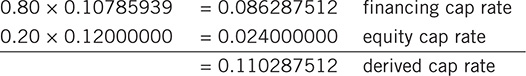
Consider the difference between $1,000 received today and invested at 5% annual interest and the same $1,000 received not today, but at the end of some later year.
Clearly, the longer you have to wait to receive the money, the greater your opportunity cost. In this example, it costs you $50 to wait one year, but by the end of year 5, the cost of waiting has grown to $276. Now you know why banks charge interest on mortgages.
To understand the concept of present worth, or present value (PV) as it is commonly called, you just need to look at this chart from a slightly different perspective. Let’s simplify it a bit for illustration.
If 5% per year is what you can earn with your $1,000, then at the end of year 5, you will have $1,276. In other words, having $1,276 in five years is equivalent to having $1,000 today. So, the present worth—the value today—of $1,276, due in five years and discounted at 5% per year, is $1,000.
Of course, with real estate, you typically do more than just buy today and then sell at some later date to recover your initial equity plus profit. Stuff happens in between, and you usually call that stuff “cash flow.” (At least that’s what you call it when it’s positive. When it’s negative, your vocabulary may become more colorful.)
Returning to our definition, it is this “anticipated future income stream” that you will discount back to a PV. The income stream includes the cash flows that may occur each year, as well as the final cash flow, which is the sale of the property.
Your objective is to discount these cash flows, which occur in different amounts and at different times, using an appropriate discount rate, back to a single PV. How do you do that?
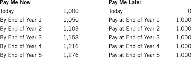
Recall the example from Chapter 3, Figure 3.6. Following the same approach you saw then, you discount the year 1 cash flow ($5,000) for a period of one year, determining its PV. Then you discount the year 2 cash flow back two years, again determining its PV. You do the same for each of the cash flows, and when you’re done, you have the PV of each of them. Finally, you add all the PVs together, and you have the present worth of the entire income stream.
If you take the cash flows shown above and discount them at 11%, you find that the PV of this income stream is $61,304.
One of the particular strengths of DCF is that it takes into account both the magnitude and the timing of your investment returns. Consider what happens if you change the timing of the cash flows in the previous example:
The total of the cash flows is exactly the same as before, but their timing is different. The PV of the series of cash flows now drops to $58,865. Why? Because you have to wait longer to receive some of the money.
In order to use PV effectively, it is essential that you pick an appropriate discount rate. Remember our last example of the five cash flows? When you discounted them at 11%, you found them to be worth $58,865. If you were to take those same cash flows and discount them at 15%, their value would drop to $49,919.
How do you choose a discount rate? Recall that we said that discounting future cash flows compensates for the cost of a lost opportunity. By investing your money in this property, you don’t have it available to invest somewhere else. The most suitable discount rate, therefore, is the one that best describes the lost opportunity. Your discount rate should be the rate of return that you could reasonably expect to achieve by investing the same amount of money in a similar investment posing a comparable risk. If other properties of this kind are typically returning 11%, then those properties are competing for your investment dollar, and 11% is an appropriate discount rate for you to use with this property as well.
In our definition, we stated that the discount rate should be applied to the income stream. What you mean by “income stream,” however, may vary according to your purpose.
In the preceding examples, we’ve been using the term “cash flow” to describe the income stream. However, an appraiser will typically define the income stream as the NOI for each year of the holding period, plus the eventual gross selling price (called the reversion) in the year of resale. By using NOI and gross selling price, the appraiser is trying to estimate the value of the property in terms of its ability to produce income, independent of any financing or income tax considerations.
An investor may prefer to find the PV of the actual cash flows instead, as we did in our examples. By this, we mean the cash flow after taxes for each year of the holding period, plus the net sale proceeds after taxes in the year of resale.
If you discount these cash flows, you are looking not at the value or price of the overall property, but rather at the value of your initial cash investment, your initial equity. What did you buy with the actual cash you invested? You bought a series of after-tax cash flows occurring in the future. If you discount those future cash flows, then you learn how much they’re worth today. You already know what you paid for them—your cash investment—so now you’ll know if you got more or less than you paid for, or perhaps exactly the same.
The discounting of cash flows does take into consideration the effects of leveraging the investment through mortgage financing. If you discount the after-tax cash flows, then you can take into account the investor’s income tax expense or benefit as well. The more financing you have, the less cash you must invest. At the same time, the more financing, the less cash flow you are likely to have because of your greater debt service.
DCF’s PV calculation is a way for you to estimate the value of your investment (i.e., the worth of the income stream). It takes into account the time value of money, the occurrence of periodic cash flows, and the ultimate resale of the property and—if you choose—it can also incorporate the effects of financing and taxation.
This is a substantial improvement over some of the crude investment evaluation techniques you looked at previously. However, it is not a rate-of- return measure. As investors, we often feel more comfortable with a measure that lets us compare one investment opportunity with another. For that, we can estimate the internal rate of return of a series of future cash flows.
Internal Rate of Return
If you have persevered to this point, then you are poised to master a concept that often seems mysterious to investors: internal rate of return.
Internal rate of return (IRR) holds a dubious distinction in the panoply of investment measures. It is the most widely used and oft-quoted rate of return for real estate, and at the same time, the least understood. The next time someone claps you on the back and proclaims a property’s IRR, ask him or her, “Now just what exactly does that mean?” This writer will bet you a local suspension bridge (acquired recently in a friendly card game) that the answer, if any, will be unintelligible.
You will certainly reach an understanding of IRR more easily with a few small steps than with a giant leap. Lucky for you, the previous material provided you with just those steps.
Once again, let’s back up just enough to get a running start. We defined an investment as an expected stream of income, and we defined the PV of that investment as the sum of the discounted values of each of the future cash flows. To put it less technically: Each year, the investment throws off some sort of cash flow—positive, you hope, but negative perhaps. In the year that you dispose of your investment property, you realize one extra cash flow—the proceeds of sale.
The longer you have to wait to collect your money, the less “PV” it has today. As you’ve seen repeatedly throughout this book, there is a time value to money.
Your real estate investment will produce cash flows periodically. For the sake of simplicity, you typically estimate these future cash flows on an annual basis. A cash flow you receive today is worth its face value, but you must discount each that you expect to receive later to its lower PV. Again, the longer you wait, the bigger the discount.
If you add up the PVs of each of the future cash flows, you arrive at the PV of the entire income stream; and since the income stream represents your investment, you now have the present worth of that investment.
Look at one more example. You purchase a building today, operate it for five years, and then resell it. Here are your actual cash flows:
You also believe you should discount future cash flows by 11%. What that really means is that you think if you had this $25,000 in hand today, you could invest it for an average return of 11% per year over the next five years. You think this is true because you discover that other property investments of similar kind and risk are currently returning about 11% to their owners. You assume that for every year you don’t have one of those cash flows in hand, you’re going to lose a potential return of 11%, so that’s how much of a discount you should apply to each.
The PV of each cash flow, discounted at 11%, looks like this:
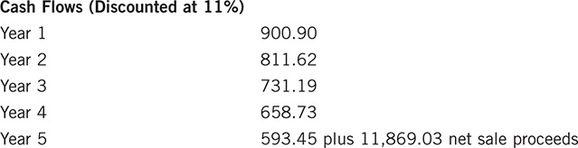
Add these all up, and you get not the $25,000 face value, but $15,564.92. That is the sum of the present worth of each of the expected future cash flows, including the resale. If you have made accurate projections of these cash flows and have selected an appropriate discount rate, then it is reasonable to say that the future economic benefit that you will derive from the property is worth about $15,565 today.
Does that mean the property itself is worth $15,565? If you pay all cash and have no other costs of acquisition (i.e., no attorney’s fees, title search, recording fees, etc.), then this would indeed be the value of the property to you as an investor seeking an 11% return. But that’s not how you usually buy property, so let’s rephrase this statement: Given these cash flows occurring at these points in time, $15,565 is how much cash you, as an investor seeking an 11% return, would be willing to invest.
The sum of the discounted cash flows always represents the value of (i.e., what you’re getting for) your cash outlay. Therefore, if you buy a property for all cash, then the sum of the discounted cash flows equals the value of the property, because that is how much cash you invest. If you finance the purchase, then the sum of the discounted cash flows represents the value of just your cash outlay.
Keep in mind, if you finance the property, you have less cash flow because you have to pay debt service; and you have less sale proceeds because you have to pay off the mortgage. It makes sense that when you discount these smaller cash flows, you get an amount that equates to your cash outlay, which itself is also less than the full property value in a leveraged investment.
At last, we get to the point. Up until now, you have assumed that you know or can project the future cash flows and the discount rate and that you will use that information to estimate the present worth of those cash flows. What if you already know the present worth of the future cash flows?
If you know the actual cash investment (the purchase price less financing and costs of acquisition), you have essentially declared, “If I make this deal on these terms, then the cash I must bring to the table is by definition the present value of the future cash flows.” But at what discount rate?
Previously, you used the future cash flows and the discount rate to figure out the PV of your investment. Now, just as in eighth grade algebra (which this definitely is not), you’re going to solve for a different variable: the discount rate. When you find it, you’re going to call it the IRR.
Let’s say this all together one more time: If I know or can project the future cash flows and the proper discount rate, I can calculate the PV of my cash investment.
If I know or can project the future cash flows and the PV (i.e., the amount) of my cash investment, I can calculate the discount rate, which I will then call the IRR.
(An aside: Do not even think of taking a series of cash flows and a cash investment and attempting to figure an IRR manually. IRR must be figured using a binary search or “successive approximations” technique that will make you forget why you wanted to know the answer in the first place. There are other painless ways to solve for an IRR: Financial calculators can do this, and so can Microsoft Excel. We provide a basic Excel model that you can download at http://www.realdata.com/book. You can also avail yourself of easy-to-use income-property analysis software, such as that provided by RealData.)
IRR is superior to most other measures of investment quality because it takes into account both the magnitude and the timing of every cash flow. A difficult concept to grasp at first, it is elegantly direct. Discount all future cash flows from the point in time when they occur back to the present using a single discount rate. When you find the unique rate that makes the sum of these discounted cash flows equal to the initial cash investment, you have found the IRR.
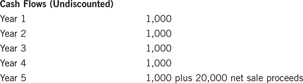
Let’s use the data from the previous example to try some IRR computations. You can use an Excel model that applies the IRR function to a series of cash flows:
(This model is available for you to download at http://www.realdata.com/book.) In each of the first four years you have a positive cash flow of $1,000.
In year 5, you have combined cash flow and sale proceeds of $21,000. Let’s say that your initial cash investment is $15,565. Enter these amounts into the model:
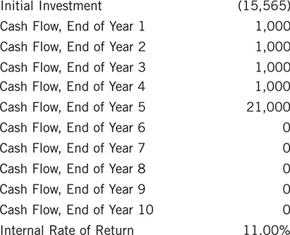
Your IRR is exactly 11%. Should you be surprised? Not at all, because this computation is really the flip side of what you did in the previous PV example. There, you had the same cash flows for years 1 to 5, but you specified a known discount rate (11%) in order to compute the PV. Here, you specify the PV (how much cash you’re going to invest) in order to compute the overall discount rate (the IRR).
It should be clear that the more you pay to get the cash flows, the lower your overall rate of return will be; and the less you pay for them, the higher your rate of return. Let’s say that you pay only $14,000:

Now you’re doing better—better in fact than the typical investor in your area, who you determined was getting 11%. What if you pay $17,000?
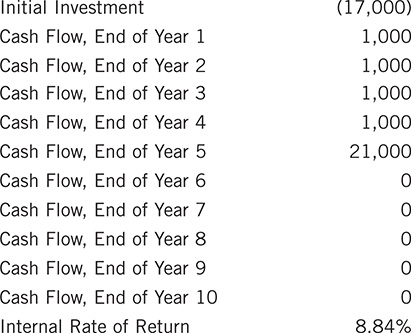
Obviously, this is much less appealing. You say to yourself, and probably to the seller, the broker, and everyone else within earshot, that if other properties are yielding 11%, you are not going to settle for 8.84%.
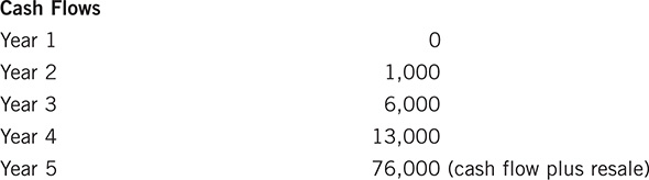
But wait, there’s more to this story. You’ve been zoned in on this idea of holding the property for five years. What if you hold it for more than five years or for less? Now you’ll need to come up with some additional forecasts about cash flow beyond five years and about the selling price in years other than 5. In real life, the following might not occur, but let’s make these following assumptions, both to keep things simple and to illustrate an important point about IRR: Stick with the $17,000 cash investment that made you so cranky in the last example. Say also that the annual cash flow will always be $1,000 and the resale price will be $20,000, no matter when you sell. Doing so will allow you to isolate your attention on the subject of timing. Try selling the property two years earlier than before (i.e., end of year 3) and two years later (end of year 7).
The following is end of year 7:
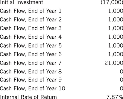
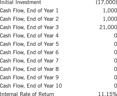
So what happened? Clearly, your cash flow is not an impressive number with this property; the resale is where the payoff occurs. If you postpone that resale by another two years out to year 7, then the proceeds represent even less to you in current dollars, and your IRR on this investment drops. On the other hand, if you can accelerate your receipt of the big payoff, then those proceeds are worth more to you in current dollars, and your IRR increases. In fact, it increases to about 11%, making this look like a tolerable deal if you don’t hold beyond the three-year horizon.
What usually happens, of course, is that neither the cash flows nor the potential sale proceeds remain static. Cash flows may bounce around a bit (more repairs one year than another, for example), but in general, you expect the trend to be upward over time. And you certainly expect the potential cash proceeds from selling the property to grow over the years, as the value of the property increases because of increasing NOI and the mortgage balance goes down.
IRR packs more analytical power than most other measures of investment quality you have seen so far, primarily because of its sensitivity to both the timing and the magnitude of cash flows. Now is when you can really start having some fun with the numbers and using their power to guide you to good investment decisions. Using the cash flows and the potential resale proceeds, for example, you could figure the IRR if you held the property for one year and then sold it, or for two years or three and so on.
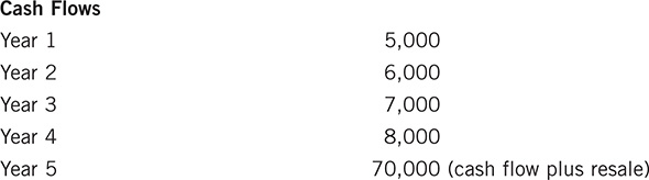
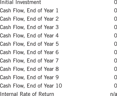
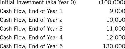
Let’s say that you run a five-year forecast on an income property, including a possible sale of the property in each of those years, and you get the following IRRs:
![]()
What you observe here is that the IRR peaks in the third year. In other words, if you operate the property as planned and sell it at the end of three years, again as planned, your rate of return for that period of time would be higher than the rate for any other holding period. In a situation like this, IRR is more valuable than a simple rate-of-return calculation. If the IRR peaks, it is identifying an optimum holding period. Investors who don’t understand IRR often complain, “This makes no sense. My IRR peaks at the end of year 3. But my cash flow from operations is going up in years 4, 5, and beyond, and so is the resale value of the property. How can the IRR go down when everything else is going up?”
It can; it often does; and it shouldn’t be ignored. Picture this: You buy a property and successfully turn it around. In the first three years of ownership, you upgrade it physically, improve its management, and bring its rent roll up dramatically. Once it is stabilized and running like a top with all leases at market rents, you continue to enhance the income, but at a more modest consumer-price-index rate of growth.
So why does the IRR go down after year 3? Remember that the IRR is sensitive to the timing and magnitude of cash flows. For the first three years, you moved the cash flow from operation and the potential cash proceeds from resale up at an impressive rate. In the fourth year, you moved them up again, but at a significantly lesser amount. Keep in mind that the big cash flow increases came early, so they were especially valuable—it’s that time value of money again, where these cash flows are discounted less severely because they occur earlier. Not only are the later cash flow increases smaller, but they are going to be discounted over a greater number of years. If you hold the property for four years instead of three, that fourth year dilutes the overall rate of return because (a) it wasn’t as strong as each of the first three, and (b) it had to be discounted even more because it occurred yet another year later.
None of the later years in this example can match the performance of the first three, so every additional year of holding the property decreases further the overall return. In this analysis, the IRR is capable of delivering a very powerful and perhaps surprising message: “Don’t be fooled by the fact that you show cash flow increases every year. You made your biggest impact in the first three years. That’s when you should consider cashing out and doing this all over again somewhere else.”
Now that you’ve mastered cash flow and resale and IRR, you don’t have to look just for an optimum holding period. What happens to your IRR if you take a bigger mortgage and use less cash? What happens if you do the opposite? What if you spend money for improvements that allow you to raise rents—will that boost your return or reduce it?
This sounds terrific; you’ve apparently found the perfect way to measure your investment’s return. But wait—the standard implementation of IRR has a few warts. Sometimes its results are imperfect, sometimes even misleading. Let’s turn next to the potential problems with IRR and to some potential solutions.
Financial Management Rate of Return and Modified Internal Rate of Return
As the last section concluded, you reached an epiphany of sorts. You turned discounted cash flow on its head, solving for the rate rather than the present value. That rate—the internal rate of return—looked like it provided an excellent measure of investment return and a promising way to compare alternative investments because it was sensitive to the interplay between the timing and the magnitude of your investment’s cash flows.
At last, with IRR, you had a measure that was a considerable improvement over static metrics like cash-on-cash return and gross rent multiplier, and one that was probably more informative than net present value (NPV).
Like all good mystery writers, however, I try always to have one or two good chapters left in the hole, bringing you back for more. Yes, there is a bit more to the story.
IRR is great, and most investors are quite comfortable using it. But even the venerable IRR has its critics. What are the problems with IRR, and how might you tweak it to overcome those problems?
The Problems with IRR
Straight-up internal rate of return works well in many situations, but not quite all. In the typical investment, you expect to have a single negative cash flow on day 1 to acquire the investment, perhaps followed by a series of periodic positive cash flows. The last of these will be the proceeds of sale when you finally dispose of the investment. In such a scenario, IRR usually works well and is quite intuitive. Take this typical series of cash flows:
Perform an IRR calculation here, and you’ll get 13.36%.
Things get a little dicey when your cash flows lose their comfortable regularity. Particularly vexing is a situation where your investment timeline expects to encounter some negative cash flows. Perhaps you’re projecting a significant increase in the interest rate on your financing; or you expect to have some major (but unfunded) repairs; or you want to play “what if … ?” to see what will happen if you lose an important tenant and cannot replace that tenant quickly. Any of these possibilities could throw your projected cash flow for a future year into the negative.
That’s where the arcane math behind IRR throws you a curve. In general, if you have more than one change of sign in the series of cash flows (and you must include the initial investment as one of the cash flows), then you may encounter “nonunique” results. “Nonunique” is a polite way of saying the same set of facts can give you more than one answer, which clearly is not helpful.
Consider this example from the classic text Mastering Investment Real Estate (Messner, Schreiber, Lyon, and Ward, Realtors National Marketing Institute, 1982):
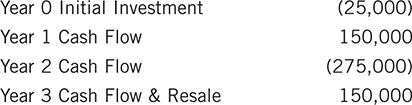
In this series of cash flows, the sign changes three times; therefore, there could be as many as three different internal rates of return, i.e., rates at which you could discount these cash flows so that their net present value would equal zero. Indeed, there are three such rates: 0%, 100%, and 200%, and they’re all mathematically correct.
The IRR is of little value if it presents you with multiple solutions for the same set of data and invites you to pick the one you like.
If IRR’s relationship with negative cash flows is occasionally dysfunctional, it doesn’t get along as well as it should with positive cash flows either. Conventional wisdom has long held that IRR assumes that positive cash flows can be reinvested until the end of the holding period at the same rate as the IRR itself. You will, of course, reinvest positive cash flows at the best rate you can reasonably obtain, and that rate is likely to be closely tied to the size of the cash flow. If your cash flow is large, you may be able to reinvest it in another piece of real estate. If it is small, then passbook savings may be your only option. The more that the calculated IRR exceeds your actual reinvestment rate, the more likely it is that the IRR will overstate the property’s return—often by just a little, but given the right set of figures, potentially by a lot. What’s an investor to do?
In order to take this discussion to the next level, you’ll need to add two new terms to your investment lexicon:
Safe rate (sometimes called the finance rate). This is the interest rate at which you put money aside, in a secure and reasonably liquid form, so that it can grow to meet the amount or amounts needed to cover future negative cash flows. The rate from a money market or short-term certificate of deposit might be an appropriate choice for the safe rate. In computing FMRR and MIRR, discussed below, the safe rate is used to discount negative cash flows back in time—to a previous positive cash flow in FMRR or to the time when you make your initial investment and acquire the property (year 0) in MIRR—effectively determining how much cash you would have to set aside at that given time so that the cash could grow in interest to be exactly what you need to absorb the negative cash flow when it occurs.
For example, if you predict a negative cash flow of $15,000 at the end of year 1 and could put cash aside in a secure and liquid form at a 4% safe rate when you make your initial investment, then the amount you would need to set aside is $14,423. Check the math:
14,423 × 0.04 = 577 (the interest you earn in one year)
14,423 + 577 = 15,000
Reinvestment rate (sometimes called the risk rate). This is the rate at which you assume you can reinvest all positive cash flows. As discussed above, the internal rate of return presumes that you can reinvest positive cash flows at the same rate that the property yields (i.e., at the IRR). Often this is not true, especially when cash flows are too small to reinvest in a comparable piece of real estate.
Financial Management Rate of Return
You can use modified versions of IRR to deal with the problems of nonunique results and reinvestment of positive cash flows. Back in the ’70s (the 1970s, that is), when this writer was a young investor in bell-bottom pants, the technique was called financial management rate of return (FMRR).
FMRR eliminates negatives by first discounting them back at the safe rate to the nearest previous positive cash flow, then adding that discounted negative amount to the positive cash. If there are any negative amounts left over after doing this, those are discounted back to the time you make your initial investment (i.e., year 0), also at the safe rate, and added to the initial investment. The procedure then compounds the remaining positive cash flows forward to the end of the holding period at a rate that is realistic for those cash flows. It is up to you, the analyst, of course, to specify the safe and reinvestment rates.
This process leaves you with a revised string of cash flows on which you can perform a proper IRR, a series that begins with a negative amount when you make your initial cash investment, ends with a positive amount when you dispose of the property, and presents all zeros for the intermediate cash flows.
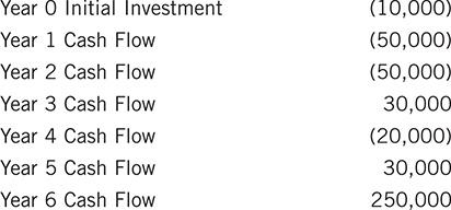
For example, say that you found these among your series of cash flows:
![]()
If your safe rate were 4%, you would discount the (20,000) year 4 cash flow back one year at that rate. The result would be (19,231). Now in year 3 you can combine the positive 30,000 with the negative (19,231) and at the same time eliminate the negative cash flow in year 4.
![]()
Modified Internal Rate of Return
At some point, perhaps in the mid-’80s, this writer observed that most investors and brokers were using a variation of this variation on IRR called modified internal rate of return (MIRR). I can only speculate about what caused this shift, but I have a theory. Microsoft published its Excel spreadsheet software with MIRR as a built-in function. MIRR is perhaps slightly less precise than FMRR, but I suspect that it demands less computing power to calculate. The difference with MIRR is that it discounts all negative cash flows to year 0 rather than trying to mix and match individual negatives with offsetting positives. The difference between it and FMRR is typically slight.
Consider these cash flows, once again based on an example in the text by Messner et al.:
If you use a safe rate of 5% to discount negative cash flows, use a reinvestment rate of 10% for positive cash flows, and perform the admittedly tedious task of figuring the FMRR, you will find that your FMRR equals 19.4%. Use Excel’s MIRR function with the same safe and reinvestment choices, and the result is 18.0%. Probably close enough for government work.
It’s worth noting, however, that if you were to use Excel’s IRR function on these cash flows, using a “guess” rate of 20% to narrow the field of possible answers, you would get an IRR of 25.2% for these same cash flows. Clearly, the difference in this example between IRR and MIRR is quite meaningful. The MIRR yields a more conservative and probably more realistic measurement.
Capital Accumulation Comparison
While FMRR and, more practically, MIRR address the chief deficiencies of IRR as a measure of return, they can still come up a bit short when you want to compare mutually exclusive investment alternatives. The problem here is in accounting for both the duration and the scale of your competing options. Using MIRR to compare opportunities that require the same initial investment and that will be held for the same length of time seems reasonable enough. But what if the alternatives require different amounts of cash or presume different holding periods?
Let’s say that you want to decide between two properties, one requiring a cash investment of $100,000, the other $60,000. Clearly, you must really have $100,000 in hand if you’re considering both options. To make an “apples-to-apples” comparison, you should invest $100,000 no matter which property you choose. When considering the property that requires only $60,000, your analysis should involve both the return you expect to receive from the property and the return you expect from the remaining $40,000 cash that you were free to invest elsewhere.
Likewise, if you project that you will hold one property for four years but the other for five, you should look at the final proceeds from the four-year property and take into account the return you could earn with those proceeds if you invested them elsewhere for one more year. In other words, when comparing two investment alternatives, you should try to equalize the holding periods.
That brings us to capital accumulation, aka accumulation of wealth. Properly speaking, a capital accumulation (CpA) comparison is not a rate-of-return measurement. However, it is a way you might address the issue of choosing among mutually exclusive investments that may require different amounts of up-front cash and involve different holding periods. This method allows you to compare these investment alternatives not with a rate-of-return percentage but rather in terms of accumulated dollars, even if those dollars don’t remain in the particular investment for the entire time.
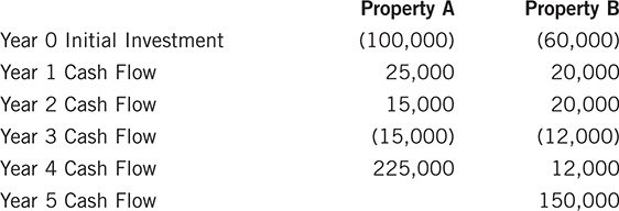
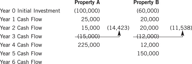
Consider two mutually exclusive investment opportunities, Property A and Property B, with the following cash flows:
To perform a capital accumulation comparison, you begin by eliminating the negative cash flows, as you saw in the FMRR example above. Let’s say you choose a safe rate of 4%.
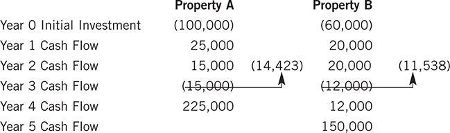
You have effectively eliminated the negative cash flows from year 3 and promoted them as discounted amounts, which you will absorb into year 2.
Next, you compound all positive cash flows to the end of your longest holding period, year 5. You decide on a reinvestment rate of 9%.
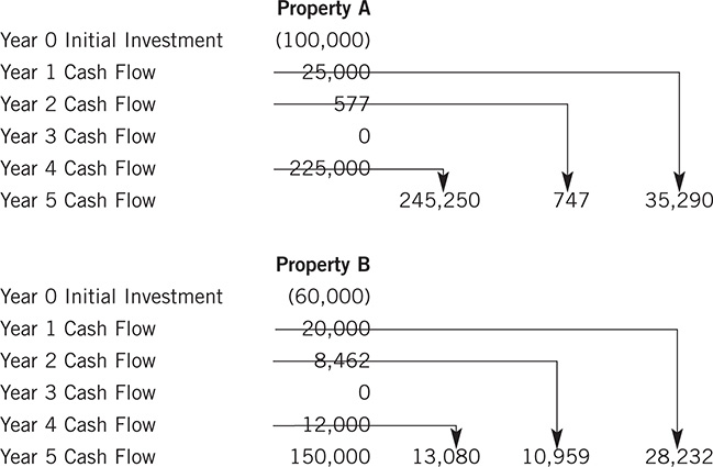
Note what you’ve done with Property A. Even though you expect to sell it at the end of year 4, you are comparing it with a property that you plan to sell at the end of year 5. To make a proper comparison, you must say to yourself, “I need to keep my money invested until the end of year 5, no matter which property I choose.” To do that, you’ll take your year 4 cash flow, which includes the sale proceeds, and invest it all for one more year at your reinvestment rate.
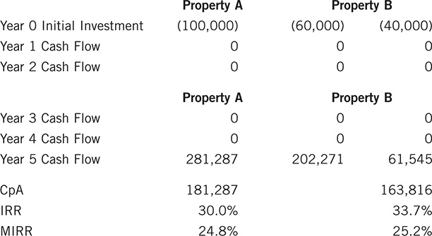
You have one last consideration to deal with: Clearly, you must be starting out with $100,000 cash in your pocket, or you wouldn’t be considering the purchase of Property A. If you decide to buy Property B, then you’ll have $40,000 left over to work with. To make a true comparison of these alternatives, you need to commit the same amount with either choice. You do that by assuming that you’ll invest the remaining $40,000 for the five-year holding period at your reinvestment rate of 9%.
Your final series of cash flows, after discounting negatives and compounding positives, looks like this:
Let’s have an instant replay of what you did here, first using just Property A. If some of this is starting to sound familiar, you’ve probably noticed that this process of computing CpA looks a great deal like what you saw for FMRR above, except instead of looking for a rate of return, you’re looking for a total accumulation of cash.
In the example, you first needed to eliminate the negative cash flow of $15,000 that occurred in year 3. You did that by discounting it back at 4% per year until its discounted amount could be absorbed by an earlier positive cash flow. In this case you had to go back only one year. Negative 15,000 discounted at 4% for one year is negative 14,423, which could be absorbed by year 2’s positive 15,000, leaving a net for year 3 of the difference, 577.
(If you had some amount of negative cash flow that you could not absorb into positive cash flows, you would discount the negative cash back to year 0 and add it to the initial investment amount, again as described in FMRR.)
Next you compounded each of Property A’s positive cash flows forward to year 5 at the reinvestment rate of 9%. Why five years when you expect to hold the property for just four? Because you’re comparing Property A with an alternative and mutually exclusive investment that you would hold for five years. So to keep the alternatives in balance, you needed to keep your end of year 4 money in play at the reinvestment rate for the same amount of time as in Property B.
When you were done, your entire accumulation was a combined negative 100,000 and positive 281,287, or 181,287.
Property B worked the same way but required one additional step: equalizing your cash commitment by investing elsewhere the $40,000 that was not needed to purchase Property B. By investing that $40,000 at the reinvestment rate, you were able to compare two investment scenarios, each requiring $100,000 of cash.
As you can see, the total capital accumulation for Property A ($181,287) is greater than that for Property B ($163,816), so Property A is your preferred choice. Interestingly enough, if you were to do an IRR on the original cash flows, you would find that Property B’s IRR, with 33.7%, is greater than Property A’s 30.0%, while Property B’s MIRR of 25.2% wins by a nose over Property A’s 24.8%.
Why might that be so? The answer should lie in one or both of the “equalizing” factors: holding period or initial investment. Perhaps, in this example, $40,000 is working harder for you when invested in Property A than invested independently if you chose Property B.
You can use the capital accumulation comparison to weigh more than two alternatives, of course; and although our focus here is on real estate, there may come a time when you’d like to consider a non–real estate option (would that be an unreal opportunity?).
Let’s expand the example above to include a third possible choice. Your best friend asks you to loan him $90,000 at 12% for six years so he can invest in a chinchilla ranch. You question the wisdom of his plan, but he’s itching to invest, so you agree to consider the loan, subject to a capital accumulation comparison along with the two investment properties you are currently considering.
This gives you an opportunity to practice your CpA skills a bit more because you’ll need to extend your horizon for all three investment options to six years to match the term of the loan.
You start by calculating the cash flows for the six years of the loan: A loan for $90,000 at 12% for 72 months requires a monthly payment of $1,759.52, or approximately $21,114 per year.
Your three investment options stack up like this:
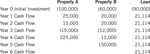
For Properties A and B, the discounting of the negative cash flows from year 3 will be exactly the same as in the original example; the addition of a sixth year has no impact here:
However, the compounding of positive cash flows will be different from before because, in order to compare the cash flows for the properties with that for the six-year loan, you must treat each initial cash investment as if it were kept in play for six years.
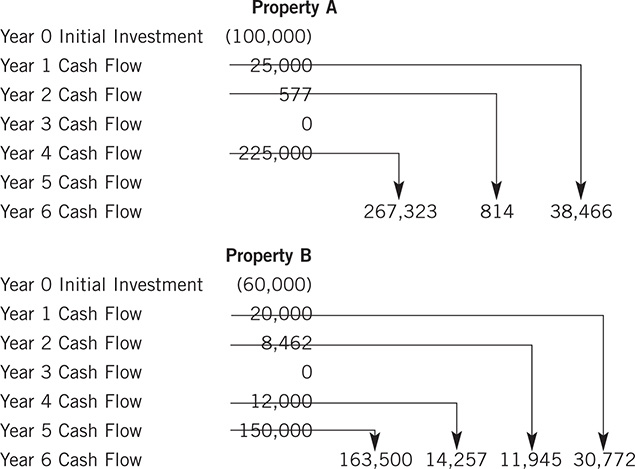
Note that each of these positive cash flows grows to a slightly larger amount than it did in the previous example, because each is being reinvested for an additional year.
Add it all up, and your capital accumulation if you hold these properties for six years instead of five looks like this:
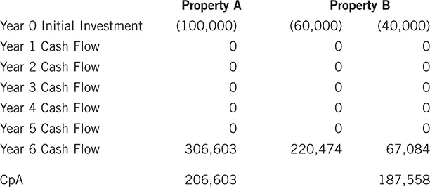
Of the two real estate investments, Property A remains the preferred choice. Now you can see how you fare with the money you’re lending, reinvesting the payments you receive (i.e., your positive cash flows) at 9%:
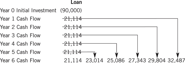
The five reinvested cash flows from years 1 through 5 combine with the year 6 amount to give you a total of $158,848 in the sixth year.
Remember that you used only $90,000 in making this loan, so you still have $10,000 left to invest. After you invest this extra cash for six years at the 9% reinvestment rate, your capital accumulation for this third option ends up as follows:
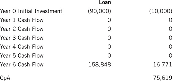
The CpA for this loan is clearly lower for either of the two real estate opportunities. You’re going to have to find some way to tell your friend that you can’t finance that chinchilla ranch.
You’ve come a long way from GRMs and payback periods. Now you understand how the key elements of a real estate investment interact. You understand the time value of money, the discounting of cash flows, the benefits and shortcomings of IRR, and even more advanced measures such as modified IRR and capital accumulation. Success comes to real estate investors who work the numbers to find and structure the best deals.