
8
Overview of Distributed Decision Fusion
Martin E. Liggins*
CONTENTS
8.2 Single Node Detection Fundamentals
8.3.1 Optimizing Local Decision Managers (Step 1)
8.3.2 Optimizing Fusion Rules (Step 2)
8.1 Introduction
The concept of distributed detection fusion† or decision fusion has evidenced wide interest over the past 25 years, beginning with applications ranging from multimode signal detection and distributed multisensor decision theory to multiple change detection algorithms for surveillance imaging systems to subordinate team decision managers or decision makers (DMs) within a command and control formulation. Recent applications have involved team-decision concepts for wireless networks and particle swarm theory for biometric security systems.
Distributed detection fusion problems are often represented as optimization problems involving a composite collection of local DMs (involving sensors, algorithms, control processes, and persons) feeding a centralized (global) DM. As we embrace the ever-growing challenge of network-centric systems, the need and the opportunity now exist to communicate between any number of local DMs, providing distributed interaction between local DMs within a region or between global managers. With this emphasis on network-centric development, demand for optimal decision techniques would need to grow as well.
This chapter provides the basic concepts of distributed detection fusion, beginning with the concepts of classical detection theory portrayed by Van Trees.1 We will discuss the most basic architecture—a parallel fusion architecture—and in doing so, lay out the means to develop and design system decision fusion rules. Finally, we will provide a discussion on fusion rules and the assumptions placed on local DMs.
The structure of this chapter is as follows: Section 8.2 provides the fundamental concepts of detection fusion theory, beginning with a single DM. We build on this approach to extend to multiple DMs operating within a parallel fusion system in Section 8.3, based on the concepts of team-decision theory. Section 8.4 provides an analysis of some of the common fusion rules, how they are constructed, and their performance.
8.2 Single Node Detection Fundamentals
In developing an optimal detection approach for distributed DMs, we consider the binary hypothesis testing problem for N local DMs. Consider each DM having to select between two hypotheses, H1 and H0, with known prior probabilities for each hypothesis. These hypotheses represent observations, indicating acceptance (H1) or rejection (H0) of the existence of, say, a target versus noise, correct versus false target classification, or detecting relevant anomaly detections over that of random activity.
Consider Figure 8.1. When sensors monitor their environment, either they observe an entity of interest, Z1, and the local DM declares H1 (e.g., detect the target), or they detect noise (no target), with the local DM declaring H0 with some statistical basis. It is assumed that these choices represent the total observation space as the union of the observations, Z = Z1 ∪ Z0, with no overlap between the observation subspaces, that is, Z1 ∩ Z0 = ϕ.

FIGURE 8.1
Distributed detection fusion concept.
To develop the concepts of minimum risk associated with making a decision on a target, consider an individual DM generating a decision, ui, representing one of the two hypotheses based on its observation, yi:
H0:yi = ni (noise only)
H1:yi = r + ni (target plus noise)
The noise and signals observed by each DM are considered to be statistically independent from any other DM. Decisions characterized by each DM, ui, are dependent on both the observation and a threshold. We can denote these decisions as follows:
This detection performance is characterized by the local DM based on a probability conditioned on choosing the true hypothesis, P(ui|Hj). Bayes formulation attributes the cost to each possible choice with decision rules designed to minimize the cost of making a decision, that is, minimizing the expected risk, R.
For a single DM, we can express this risk as follows:
where Cij is the cost of declaring hypothesis i, given that hypothesis j is true and Pj is the prior probability representing the choice that hypothesis j is true based on the observation y. The conditional probability represents the probability that integrating over a region, Zi, will generate a correct response for a target.
Expanding over the summation gives
which reduces to
by taking advantage of the fact that Z represents the total observation space, with unity probability. Minimizing risk is equivalent to minimizing the integrand, that is, assigning y to H1 if the integrand is positive or to H0 for a negative integrand. Alternatively, we can write the integrand in the form of a likelihood ratio as follows:
where the left-hand side indicates the likelihood ratio and the right-hand side the detection threshold.
We can rewrite the risk in terms of the following well-known probabilities:
Probability of a false alarm, PF = ∫Z1 p(y|H0)dy
Probability of a detection, PD = ∫Z1 p(y|H1)dy
Probability of miss detection,
Also note that the prior probability of H1 can be written as P1 = 1 – P0.
The risk becomes
which can be reduced to
where we define the costs to be CF = P0(C10 – C00), CD = (1 – P0)(C01 – C11), and C = P0C00 + (1 – P0)C01, assuming the cost of an incorrect decision to be higher than the cost of a correct decision, that is, C10 > C00 and C01 > C11.
8.3 Parallel Fusion Network
Now consider a number of DMs within the parallel decision fusion network shown in Figure 8.1. Extending the Bayesian minimum risk concepts to a set of distributed detectors, each DM provides a localized decision and transmits results to a centralized fusion system, where they are combined into a composite result. The fusion system combines the local results by an appropriate fusion rule, and provides a final decision, u0, representing the viability that the global hypothesis represents the true hypothesis. Fused optimization of the results depends on an evaluation of the transmitted decisions from each of the N DMs and developing the appropriate fusion rule to define how individual local decisions are combined.
Varshney2, 3, 4 and 5 provides an excellent derivation. We follow a similar approach. We define the overall fused probabilities as follows:
Fused probability of a false alarm, PF = ΣuP(u0 = 1|u)P(u|H0)
Fused probability of a detection, PD = ΣuP(u0 = 1|u)P(u|H1)
where ∑u is the summation over the N DMs. Substituting these system probabilities into Equation 8.4 gives the overall risk as follows:
Tsitsiklis6, 7 and 8 points out that decentralized detection problems of this type fall within the class of team-decision problems. Once a decision rule is optimized for each local DM, the ensemble set of decisions transmitted to the fusion center represents a realization from all DMs. That is, each DM transmits ui = γ(yi) contributing to a global ensemble set u0 = γ0(u1, u2, u3, …, uN) to be evaluated at the fusion center. For conditionally independent conditions, observations of one DM are unaffected by the choice of the other DMs. Tsitsiklis shows that once the individual strategies are optimized, the overall system fusion can be represented by a person-by-person optimization approach.
Person-by-person optimization can be performed in two steps:
Likelihood rules are generated for each local DM, holding all other DMs fixed, including the fusion decision.
Fusion rule is obtained in a similar way, assuming all local DMs are fixed.
8.3.1 Optimizing Local Decision Managers (Step 1)
For the individual DMs, assume all other DMs are fixed to an optimal setting, except for the kth DM. Then from Equation 8.5, we can expand the effects of the other DMs on uk as follows:
From the total probability, P(uk = 1|Hj) + P(uk = 0|Hj) = 1, we can separate out the effect of the kth detector as follows:
where the terms in the first summation remain fixed and can be absorbed into the constant, whereas the first bracket in the second summation does not directly affect uk and can be treated as the weighted influence, α(u), on the kth detector.
Expanding to show the impact of the observations, we have P(u|Hj) = ∫YP(u|Y)p(Y|Hj)dY. Then the risk becomes
The conditional probability of the kth detector can be pulled out of the integrand because of the independence of the observations and formulated as a likelihood ratio. The optimal decision (i.e., the kth detector) is represented as follows:
For conditional independence, this reduces to the threshold test as follows:
Tenney and Sandell9 in their groundbreaking paper, point out that even for identical local detectors, the thresholds τi are coupled to the other detectors, as shown in Equation 8.8. That is, τk = f(τ1, τ2, …, τN)i≠k for each detector. Even if we have two identical detectors, the thresholds will not be the same. The impact of this is important. Individually, sensor thresholds may be required to maintain a high threshold setting to keep false alarms low, reducing the opportunity to detect low signal targets. By not requiring all sensors to keep the same high threshold, the fusion system can take advantage of differing threshold settings to ensure that increased false alarms from the lower-threshold sensors are “fused out” of the final decision while ensuring an opportunity to detect difficult targets.
8.3.2 Optimizing Fusion Rules (Step 2)
The number of possible combinations that could be received from N local DMs is 2N, assuming a binary decision. In a similar way, the fusion center uses these results to develop an overall system assessment of the most appropriate hypothesis. The goal is to continue the team-decision process to minimize the overall average risk at the fusion center. Referring back to Equation 8.5, the overall system risk becomes
Choose one decision, , as one possible realization for the set of local DMs, then the fused risk becomes
where
The risk is minimized for the fusion rule when
This provides the fusion rule:
Assuming conditional independence, we can write the overall fused system likelihood as a product of the individual local decisions:
Thus, Equation 8.8 provides 2N simultaneous fusion likelihoods that work to achieve system optimization for each local DM.
Other architectures expand on these principles. For instance, Hashemi and Rhodes,10 Veeravalli et al.,11 and Hussain12 discuss a series of transmissions over time using similar person-by-person sequential detections that use stopping criteria such as Wald’s sequential probability ratio tests. Tandem network topologies13,14 are discussed by transmitting from one DM to the neighboring manager, then the combined decisions are sent to the next neighbor, and so on. Multistage and asymmetric fusion strategies are discussed in Refs 15 and 16.
8.4 Fusion rules
The combined team-decision solution, involves solving the N local DM thresholds in Equation 8.8 simultaneously with the 2N fusion likelihoods in Equation 8.9, coupling the local and fused solutions. Thus, to achieve system optimization, the decision fusion process optimizes the thresholds for each local DM by holding the other DMs fixed, and repeating the process until all local DM thresholds are determined. The resulting thresholds are coupled to the global likelihood and solved simultaneously. Their simultaneous solution provides the basis for determining the set of fusion rules, a total set of 22N rules. Selection of the appropriate fusion rule is determined by an evaluation of all possible decisions.
Table 8.1 shows the explosive growth required to develop a complete set of fusion rules—for instance, four DMs give rise to more than 65,500 rules. However, an examination of the rule sets shows that a great many of the rules can be eliminated through the principle of monotonicity,2,17, 18, 19 and 20 while even further reduction can be made with some knowledge of the DMs.
The assumption of monotonicity implies that for every DM, PDi > PFi, and as such not all fusion rules satisfy threshold optimality. For example, consider a condition where K sensors select the primary hypothesis, H1. Under a subsequent test, if M > K sensors select hypothesis H1, where the set of M sensors includes the set of K sensors, then it is expected that the global decision provides a higher likelihood for the M sensors than for the K sensors. Choosing the fusion rule with the largest likelihood value ensures an optimal result. Alternatively, as Table 8.1 shows, any fusion rule that contradicts this process can be removed, significantly saving on the number of necessary rules to evaluate.
Figure 8.2 shows a simple but common example of a complete set of fusion rules generated for two DMs. We can gain considerable insight by examining these rules further. For example, fusion rule d1 rejects H1 regardless of the decisions of the two detectors (d1 = 0 for all combinations of u1 and u2), whereas fusion rule d16 accepts H1 under any condition (d16 = 1 for all combinations of u1 and u2). Rules d9 through d16 declare H1 when both local detectors reject H1. Also rules d3, d5, d7, d9, d11, d13, and d15 all reject H1 even though both detectors declare H1 (i.e., u1 = 1, u2 = 1). Thus monotonicity maintains that we keep six rules: γ(u) = {d1, d2, d4, d6, d8, d16}.
TABLE 8.1
Fusion Rules Based on Number of DMs
Number of DMs |
Set of Fusion Rules |
Number of Relevant Rules after Applying Monotonicity |
1 |
4 |
3 |
2 |
16 |
6 |
3 |
256 |
20 |
4 |
65,536 |
168 |
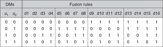
FIGURE 8.2
Global fusion rules based on two local decision makers.
Figure 8.3 shows the final fusion rule selection using two local detectors. Note that the fusion rules can be reduced even further, since d1 and d16 just bound the set of rules and are not practical. We are left with four rules: the well-known AND and OR rules, as well as rules for relying on one or the other single DM.
Much of the literature has emphasized this particular set, preferring to study the impact of AND and OR rules for their particular development. However, the case for three detectors shows a great deal more flexibility in the rule set.
Figure 8.4 shows the set of fusion rules for three detectors after we apply monotonicity, reducing the number of rules from 256 to 20. Two important additional rules become evident: “Majority Logic” and “Sensor Dominance.” For the former rule, the global decision rule requires at least two or more DMs to agree on H1 before declaring H1 at the fusion center. For Sensor Dominance, we assume that a single detector, say u2, operates with sufficient quality to be accepted by the fusion system whenever it declares H1; however, when u2 rejects the hypothesis, the other two DMs must both have positive decision before making a global declaration of H1. This condition could occur, for example, when a high quality imaging radar detects a target by itself, while two poor resolution sensors (detectors u1 and u3) must have consensus for the fusion system to declare H1.
As such, we can use this approach to eliminate some of these rules on the basis of the quality of performance of the local DMs and their sensors. For the example just discussed, we would not necessarily keep rule d34 (u1 dominates) or rule d88 (u3 dominates), since their performance quality is poorer than u2. To assess the rule set further, we would need to examine the impact of each individual detector performance on the environment and set the system fusion rules accordingly.

FIGURE 8.3
Final fusion rule selection for two decision makers.

FIGURE 8.4
Global decision rules for three detectors, applying monotonicity.
Functionally, each rule applies a different set of constraints on the basis of individual detection performance to provide the fusion system with a complete set of representative rules. Selecting the rule with the highest likelihood ensures improved target detection while reducing false alarms. If we have knowledge of the individual sensors, we can select those fusion rules that best fit their individual characteristics. Figure 8.5 shows a representative set of fusion performance curves that compare performance from three detectors against that of an individual detector. For convenience, we have assumed that all three detectors perform equally well. We can use the graph to examine the effects of the fusion rules for both fused system probability of detection (PD) as well as system probability of false alarm (PF). That is, for probability values ≥0.5 along the x-axis, we can attribute these to individual detector probability of detection (PDi), and those probability values ≤0.5 can represent individual detector probability of false alarm (PFi). The same can be considered for the fusion system performance along the y-axis. For instance, consider the two vertical lines at PDi = 0.88 and PFi = 0.10. The PD line intersects the AND rule giving a fused value of 0.6815; intersection with the OR rule occurs at PDi = 1 – (1 – 0.88)3 for a system value of 0.9983. Similarly for PFi, the AND rule gives system PF = 0.001 and the OR rule gives PF = 0.2710. From this, it appears that the OR rule can significantly outperform all other rules for PD, but at the cost of higher false alarms, whereas the AND fusion rule appears to be an excellent means of reducing PF, but provides poor overall system performance.

FIGURE 8.5
Fusion system performance in terms of individual detector performance.
Now let us consider each of the four fusion rules shown in Figure 8.5 in more detail:
The AND rule relaxes constraints on the individual detectors, allowing each detector to pass a large number of both detections and false alarms, relying on the fusion process to improve performance by eliminating most false reports. In this way, relaxed individual performance conditions will ensure improved target reportability from each detector, even though a larger set of false reports may also be developed.
The OR rule provides the reversed effect, relying on individual detectors to operate at higher detection thresholds to significantly eliminate false alarms for the fused system. This rule assumes the detectors are quite adept at distinguishing target reports from false alarms. If the detectors produce too many false reports, this rule can be detrimental. As such, a higher set of thresholds are applied to each detection source.
The Majority Logic rule falls somewhere between AND and OR performance curves, exhibiting some of the best characteristics from both strategies. It is based on the assumption that not as many false alarms would be generated by the individual detectors as in the AND case, whereas the potential to distinguish target reports from false alarms is not as stringent as in the OR case.
The Sensor Dominance rule presents an interesting case, relaxing constraints only for the single, dominant detector, expecting a lower number of false alarms for that detector, but relying on the fused element to reduce false reports from the other two poorer performing detectors. Depending on the degree of improvement of the dominant detector over the other two, system performance can improve, but false alarm performance is determined by the performance of the individual dominant detector. This rule relies on the assumption that the dominant detector is of very high quality.
Recently, particle swarm optimization theory has been suggested as an alternative to person-by-person optimization21,22 when we consider the explosive growth of rules. Here, multiple classifiers are fused at the decision level, and the particle swarm optimization techniques determine the optimal local decision thresholds for each classifier and the fusion rule, replacing the person-by-person strategy discussed in Section 8.3. Other recent trends have focused on the application of distributed fusion to wireless sensor networks.23
8.5 Summary
We have presented an introduction into the details involving the development of distributed detection fusion, beginning with the fundamentals of classical Bayesian likelihoods and extending these concepts to a parallel distributed fusion detection system, building on the concepts of system fusion rules to combine the local detectors. Each fusion rule applies a coupled decision statistic that adjusts detection performance thresholds for each DM on the basis of the combined performance of the other local detectors. We have also discussed how global fusion rules perform in terms of individual (local) detection performance, pointing out how detections and false alarms are treated on the basis of different fusion rules.
References
1. Van Trees, H.L., Detection, Estimation, and Modulation Theory, Vol. 1, Wiley, NY, 1968.
2. Varshney, P.K., Distributed Detection and Data Fusion, Springer-Verlag, NY, 1997.
3. Hoballah, I.Y. and P.K. Varshney, Distributed Bayesian signal detection, IEEE Transactions on Information Theory, 35(5), 995–1000, 1989.
4. Barkat, M. and P.K. Varshney, Decentralized CFAR signal detection, IEEE Transactions on Aerospace and Electronic Systems, 25(2), 141–149, 1989.
5. Hashlamoun, W.A. and P.K. Varshney, Further results on distributed Bayesian signal detection, IEEE Transactions on Information Theory, 39(5), 1660–1661, 1993.
6. Tsitsiklis, J.N., Decentralized detection, in Advances in Statistical Signal Processing, Vol. 2, JAI Press, Greenwich, CT, 1993.
7. Irving, W.W. and J.N. Tsitsiklis, Some properties of optimal thresholding in decentralized detection, IEEE Transactions on Automatic Control, 39(4), 835–838, 1994.
8. Tay, W.P., J.N. Tsitsiklis, and M.Z. Win, Data Fusion Trees for Detection: Does Architecture Matter, Manuscript to be Submitted, November 2006.
9. Tenney, R.R. and N.R. Sandell, Jr., Detection with distributed sensors, IEEE Transactions on Aerospace and Electronic Systems, 17(4), 501–509, 1981.
10. Hashemi, H.R. and I.B. Rhodes, Decentralized sequential detection, IEEE Transactions on Information Theory, 35(3), 509–520, 1989.
11. Veeravalli, V.V., T. Basar, and H.P. Poor, Decentralized sequential detection with a fusion center performing the sequential test, IEEE Transactions on Information Theory, 39(2), 433–442, 1993.
12. Hussain, A.M., Multisensor distributed sequential detection, IEEE Transactions on Aerospace and Electronic Systems, 30(3), 698–708, 1994.
13. Barkat, M. and P.K. Varshney, Adaptive cell-averaging CFAR detection in distributed sensor networks, IEEE Transactions on Aerospace and Electronic Systems, 27(3), 424–429, 1991.
14. Tang, Z.B. and K.R. Pattipati, Optimization of detection networks: part I—tandem structures, IEEE Transactions, Systems, Man and Cybernetics, 21(5), 1044–1059, 1991.
15. Dasarathy, B.V., Decision fusion strategies for target detection with a three-sensor suite, Sensor Fusion: Architectures, Algorithms, and Applications, Dasarathy, B.V. (ed.), Proceedings of the SPIE Aerosense, Vol. 3067, pp. 14–25, Orlando, FL, April 1997.
16. Dasarathy, B.V., Asymmetric fusion strategies for target detection in multisensor environments, Sensor Fusion: Architectures, Algorithms, and Applications, Dasarathy, B.V. (ed.), Proceedings of the SPIE Aerosense, Vol. 3067, pp. 26–37, Orlando, FL, April 1997.
17. Thomopoulos, S.C.A., R. Viswanathan, and D.K. Bougoulias, Optimal distributed decision fusion, IEEE Transactions on Aerospace and Electronic Systems, 25(5), 761–765, 1989.
18. Liggins, M.E. and M.A. Nebrich, Adaptive multi-image decision fusion, Signal Processing, Sensor Fusion, and Target Recognition IX, Kadar, I. (ed.), Proceedings of the SPIE Aerosense, Vol. 4052, pp. 213–228, Orlando, FL, April 2000.
19. Liggins, M.E. An evaluation of CFAR effects on adaptive Boolean decision fusion performance for SAR/EO change detection, Signal Processing, Sensor Fusion, and Target Recognition IX, Kadar, I. (ed.), Proceedings of the SPIE Aerosense, Vol. 4380, pp. 406–416, Orlando, FL, April 2001.
20. Liggins, M.E., Extensions to adaptive Boolean decision fusion, Signal Processing, Sensor Fusion, and Target Recognition IX, Kadar, I. (ed.), Proceedings of the SPIE Aerosense, Vol. 4729, pp. 288–296, Orlando, FL, April 2002.
21. Veeramachaneni, K., L. Osadciw, and P.K. Varshney, An adaptive multimodal biometric management algorithm, IEEE Transactions, Systems, Man, and Cybernetics, 35(3), 344–356, 2005.
22. Veeramachaneni, K. and L. Osadciw, Adaptive multimodal biometric fusion algorithm using particle swarm, MultiSensor, Multisource Information Fusion: Architectures, Algorithms, and Applications 2003, Dasarathy, B. (ed.), Proceedings of the SPIE Aerosense, Vol. 5099, Orlando, FL, April 2003.
23. Chen, B., Tong, L., and Varshney, P.K., Channel-aware distributed detection in wireless sensor networks, IEEE Signal Processing Magazine, 23(4), 16–26, 2006.
* The author’s affiliation with the MITRE Corporation is provided only for identification purposes and is not intended to convey or imply MITRE’s concurrence with, or support for, the positions, opinions, or viewpoints expressed by the author.
† It is important to point out that this work focuses on multiple sensor detection fusion. Other forms of decision fusion involving higher cognitive-based decisions such as situation awareness or impact assessment are discussed throughout this handbook.