10 Target Tracking Using Probabilistic Data Association-Based Techniques with Applications to Sonar, Radar, and EO Sensors

In tracking targets with less-than-unity probability of detection in the presence of false alarms (FA) (clutter), data association—deciding which of the received multiple measurements to use to update each track—is crucial. A number of algorithms have been developed to solve this problem.^{1, 2, 3 and 4} Two simple solutions are the strongest neighbor filter (SNF) and the nearest neighbor filter (NNF). In the SNF, the signal with the highest intensity among the validated measurements (in a gate) is used for track update and the others are discarded. In the NNF, the measurement closest to the predicted measurement is used. Although these simple techniques work reasonably well with benign targets in sparse scenarios, they begin to fail as the FA rate increases or with low observable (LO) (low probability of target detection) maneuvering targets.^5,6 Instead of using only one measurement among the received ones and discarding the others, an alternative approach is to use all of the validated measurements with different weights (probabilities), known as probabilistic data association (PDA).³ The standard PDA and its numerous improved versions have been shown to be very effective in tracking a single target in clutter.^6,7

Data association becomes more difficult with multiple targets where the tracks compete for measurements. Here, in addition to a track validating multiple measurements as in the single target case, a measurement itself can be validated by multiple tracks (i.e., contention occurs among tracks for measurements). Many algorithms exist to handle this contention. The joint probabilistic data association (JPDA) algorithm is used to track multiple targets by evaluating the measurement-to-track association probabilities and combining them to find the state estimate.³ The multiple-hypothesis tracking (MHT) is a more powerful (but much more complex) algorithm that handles the multitarget tracking problem by evaluating the likelihood that there is a target given a sequence of measurements.⁴ In the tracking benchmark problem⁸ designed to compare the performance of different algorithms for tracking highly maneuvering targets in the presence of electronic countermeasures (ECM), the PDA-based estimator, in conjunction with the interacting multiple model (IMM) estimator, yielded one of the best solutions. Its performance was comparable to that of the MHT algorithm.^6,9

This chapter presents an overview of the PDA technique and its application for different target-tracking scenarios. Section 10.2 summarizes the PDA technique. Section 10.3 describes the use of the PDA technique for tracking LO targets with passive sonar measurements. This target motion analysis (TMA) is an application of the PDA technique, in conjunction with the maximum likelihood (ML) approach for target motion parameter estimation via a batch procedure. Section 10.4 presents the use of the PDA technique for tracking highly maneuvering targets and for radar resource management. It illustrates the application of the PDA technique for recursive state estimation using the IMM estimator with probabilistic data association filter (IMMPDAF). Section 10.5 presents a state-of-the-art sliding-window (which can also expand and contract) parameter estimator using the PDA approach for tracking the state of a maneuvering target using measurements from an electrooptical (EO) sensor. This, while still a batch procedure, offers the flexibility of varying the batches depending on the estimation results.

10.2 Probabilistic Data Association

The PDA algorithm calculates in real time the probability that each validated measurement is attributable to the target of interest. This probabilistic (Bayesian) information is used in a tracking filter, the PDA filter (PDAF), which accounts for the measurement origin uncertainty.

10.2.1 Assumptions

The following assumptions are made to obtain the recursive PDAF state estimator (tracker)

There is only one target of interest whose state evolves according to a dynamic equation driven by process noise.
The track has been initialized.
The past information about the target is summarized approximately by

p [x (k) ∣ ∣ Z k + 1] = N [x (k); x ˆ (k | k - 1), P (k | k - 1)] (10.1)

$\begin{matrix} p [x (k) | Z^{k + 1}] = N [x (k); \hat{x} (k | k - 1), P (k | k - 1)] & (10.1) \end{matrix}$

where N[k(k);xˆ(k|k−1),P(k|k−1)] $N [k (k); \hat{x} (k | k - 1), P (k | k - 1)]$ denotes the normal probability density function (pdf) with argument x(k), mean xˆ(k|k−1) $\hat{x} (k | k - 1)$ , and covariance matrix P(k|k − 1). This assumption of the PDAF is similar to the generalized pseudo-Bayesian (GPB1) approach,¹⁰ where a single “lumped” state estimate is a quasi-sufficient statistic.

At each time, a validation region as in Ref. 3 are set up (Equation 10.4).
Among the possibly several validated measurements, at most one of them can be target-originated—if the target was detected and the corresponding measurement fell into the validation region.
The remaining measurements are assumed to be FA or clutter and are modeled as independent identically distributed (iid) measurements with uniform spatial distribution.
The target detections occur independently over time with known probability PD.

These assumptions enable a state estimation scheme to be obtained, which is almost as simple as the Kalman filter, but much more effective in clutter.

10.2.2 PDAF Approach

The PDAF approach uses a decomposition of the estimation with respect to the origin of each element of the latest set of validated measurements, denoted as

Z (k) = {z i (k)} m (k) i = 1 (10.2)

$\begin{matrix} Z (k) = {z_{i} (k)}_{i = 1}^{m (k)} & (10.2) \end{matrix}$

where z_i(k) is the ith validated measurement and m(k) is the number of measurements in the validation region at time k.

The cumulative set (sequence) of measurements * is

Z k = {Z (j)} k j = 1 (10.3)

$\begin{matrix} Z^{k} = {Z (j)}_{j = 1}^{k} & (10.3) \end{matrix}$

10.2.3 Measurement Validation

From the Gaussian assumption (Equation 10.1), the validation region is the elliptical region

V (k, γ) = {Z : [z - z ˆ (k | k - 1)]' S (k) - 1 [z - z ˆ (k | k - 1)] \leq γ} (10.4)

$\begin{matrix} V (k, γ) = {Z : {[z - \hat{z} (k | k - 1)]}^{'} S {(k)}^{- 1} [z - \hat{z} (k | k - 1)] \leq γ} & (10.4) \end{matrix}$

where γ is the gate threshold and

S (k) = H (k) P (k | k - 1) H (k)' + R (k) (10.5)

$\begin{matrix} S (k) = H (k) P (k | k - 1) H {(k)}^{'} + R (k) & (10.5) \end{matrix}$

is the covariance of the innovation corresponding to the true measurement. The volume of the validation region (Equation 10.4) is

V (k) = c n z | γ S (k) | 1 / 2 = c n z γ n z / 2 | S (k) | 1 / 2 (10.6)

$\begin{matrix} V (k) = c_{n_{z}} {| γ S (k) |}^{1 / 2} = c_{n_{z}} γ^{n_{z} / 2} {| S (k) |}^{1 / 2} & (10.6) \end{matrix}$

where the coefficient c_nz depends on the dimension of the measurement (it is the volume of the n_z-dimensional unit hypersphere: c₁ = 2, c₂ = π, c₃ = 4π/3, etc.).

10.2.4 State Estimation

In view of the assumptions listed, the association events

θ i (k) = {{Z i (k) is the target-originated measurement} {none of the measurements is target originated} i = 1, ..., m (k) i = 0 (10.7)

$\begin{matrix} θ_{i} (k) = {\begin{matrix} {\begin{matrix} Z_{i} (k) is the target-originated measurement \end{matrix}} & i = 1, ..., m (k) \\ {none of the measurements is target originated} & i = 0 \end{matrix} & (10.7) \end{matrix}$

are mutually exclusive and exhaustive for m(k) ≥ 1.

Using the total probability theorem¹⁰ with regard to the events given in Equation 10.7, the conditional mean of the state at time k can be written as

x ˆ (k | k) = = = E [x (k) Z k] Σ i = 0 m (k) E [x (k) ∣ ∣ θ i (k), Z k] P {θ i (k) ∣ ∣ Z k} Σ i = 0 m (k) x ˆ i (k | k) β i (k) (10.8)

$\begin{matrix} \hat{x} (k | k) = & E [x (k) Z^{k}] \\ = & Σ_{i = 0}^{m (k)} E [x (k) | θ_{i} (k), Z^{k}] P {θ_{i} (k) | Z^{k}} \\ = & Σ_{i = 0}^{m (k)} {\hat{x}}_{i} (k | k) β_{i} (k) (10.8) \end{matrix}$

where xˆi(k|k) ${\hat{x}}_{i} (k | k)$ is the updated state conditioned on the event that the ith validated measurement is correct, and

β i (k) = Δ P {θ i (k) | Z k} (10.9)

$\begin{matrix} β_{i} (k) \overset{Δ}{=} P {θ_{i} (k) | Z_{k}} & (10.9) \end{matrix}$

is the conditional probability of this event—the association probability, obtained from the PDA procedure presented in Section 10.2.7.

The estimate conditioned on measurement i being correct is

x ˆ i (k | k) = x ˆ (k | k - 1) + W (k) v i (k) i = 1, ..., m (k) (10.10)

$\begin{matrix} \begin{matrix} {\hat{x}}_{i} (k | k) = \hat{x} (k | k - 1) + W (k) v_{i} (k) & i = 1, ..., m (k) \end{matrix} & (10.10) \end{matrix}$

where the corresponding innovation is

v i (k) = z i (k) - z ˆ (k | k - 1) (10.11)

$\begin{matrix} v_{i} (k) = z_{i} (k) - \hat{z} (k | k - 1) & (10.11) \end{matrix}$

The gain W(k) is the same as in the standard filter

W (k) = P (k | k - 1) H (k)' S (k) - 1 (10.12)

$\begin{matrix} W (k) = P (k | k - 1) H {(k)}^{'} S {(k)}^{- 1} & (10.12) \end{matrix}$

because conditioned on θ_i(k), there is no measurement origin uncertainty.

For i = 0 (i.e., if none of the measurements is correct) or m(k) = 0 (i.e., there is no validated measurement)

x ˆ 0 (k | k) = x ˆ (k | k - 1) (10.13)

$\begin{matrix} {\hat{x}}_{0} (k | k) = \hat{x} (k | k - 1) & (10.13) \end{matrix}$

10.2.5 State and Covariance Update

Combining Equations 10.10 and 10.13 with Equation 10.8 yields the state update equation of the PDAF

x ˆ (k | k) = x ˆ (k | k - 1) + W (k) v (k) (10.14)

$\begin{matrix} \hat{x} (k | k) = \hat{x} (k | k - 1) + W (k) v (k) & (10.14) \end{matrix}$

where the combined innovation is

v (k) = Σ i = 1 m (k) β i (k) v i (k) (10.15)

$\begin{matrix} v (k) = Σ_{i = 1}^{m (k)} β_{i} (k) v_{i} (k) & (10.15) \end{matrix}$

The covariance associated with the updated state is

P (k | k) = β 0 (k) P (k | k - 1) + [1 - β 0 (k)] P c (k ∣ ∣ k - 1) + P ˜ (k) (10.16)

$\begin{matrix} P (k | k) = β_{0} (k) P (k | k - 1) + [1 - β_{0} (k)] P^{c} (k | k - 1) + \tilde{P} (k) & (10.16) \end{matrix}$

where the covariance of the state updated with the correct measurement is³

P c (k | k) = P (k | k - 1) - W (k) S (k) W (k)' (10.17)

$\begin{matrix} P^{c} (k | k) = P (k | k - 1) - W (k) S (k) W {(k)}^{'} & (10.17) \end{matrix}$

and the spread of the innovations term (similar to the spread of the means term in a mixture)¹⁰ is

P ˜ (k) = Δ W (k) [Σ i = 1 m (k) β i (k) v i (k) v i (k)' - v (k) v (k)'] W (k)' (10.18)

$\begin{matrix} \begin{matrix} \tilde{P} (k) \overset{Δ}{=} & W (k) \end{matrix} [Σ_{i = 1}^{m (k)} β_{i} (k) v_{i} (k) v_{i} {(k)}^{'} - v (k) v {(k)}^{'}] W {(k)}^{'} & (10.18) \end{matrix}$

10.2.6 Prediction Equations

The prediction of the state and measurement to k + 1 is done as in the standard filter, that is,

x ˆ (k + 1 | k) = F (k) x ˆ (k | k) (10.19)

$\begin{matrix} \hat{x} (k + 1 | k) = F (k) \hat{x} (k | k) & (10.19) \end{matrix}$

z ˆ (k + 1 | k) = H (k + 1) x ˆ (k + 1 | k) (10.20)

$\begin{matrix} \hat{z} (k + 1 | k) = H (k + 1) \hat{x} (k + 1 | k) & (10.20) \end{matrix}$

The covariance of the predicted state is, similarly,

P (k + 1 | k) = F (k) P (k | k) F (k)' + Q (k) (10.21)

$\begin{matrix} P (k + 1 | k) = F (k) P (k | k) F {(k)}^{'} + Q (k) & (10.21) \end{matrix}$

where P(k|k) is given by Equation 10.16.

The innovation covariance (for the correct measurement) is, again, as in the standard filter

S (k + 1) = H (k + 1) P (k + 1 | k) H (k + 1)' + R (k + 1) (10.22)

$\begin{matrix} S (k + 1) = H (k + 1) P (k + 1 | k) H {(k + 1)}^{'} + R (k + 1) & (10.22) \end{matrix}$

10.2.7 Probabilistic Data Association

To evaluate the association probabilities, the conditioning is broken down into the past data Z^k–1 and the latest data Z(k). A probabilistic inference can be made on both the number of measurements in the validation region (from the clutter density, if known) and on their location, expressed as

β i (k) = P {θ i (k) ∣ ∣ Z k} = P {θ i (k) ∣ ∣ Z (k), m (k), Z k - 1} (10.23)

$\begin{matrix} β_{i} (k) = P {θ_{i} (k) | Z^{k}} = P {θ_{i} (k) | Z (k), m (k), Z^{k - 1}} & (10.23) \end{matrix}$

Using Bayes’ formula, the Equation 10.23 is rewritten as

β i (k) = 1 c p [Z (k) ∣ ∣ θ i (k), m (k), Z k - 1] p {θ i (k) ∣ ∣ m (k), Z k - 1} i = 0, ..., m (k) (10.24)

$\begin{matrix} \begin{matrix} β_{i} (k) = \frac{1}{c} p [Z (k) | θ_{i} (k), m (k), Z^{k - 1}] p {θ_{i} (k) | m (k), Z^{k - 1}} & i = 0, ..., m (k) \end{matrix} & (10.24) \end{matrix}$

The joint density of the validated measurements conditioned on θ_i(k), i ≠ 0, is the product of

The (assumed) Gaussian pdf of the correct (target-originated) measurements
The pdf of the incorrect measurements, which are assumed to be uniform in the validation region whose volume V(k) is given in Equation 10.6

The pdf of the correct measurement (with the P_G factor that accounts for restricting the normal density to the validation gate) is

p [z i (k) ∣ ∣ θ i (k), m (k), Z k - 1] = P - 1 G N [z i (k); z (k | k - 1), S (k)] = P - 1 G N [v i (k); 0, S (k)] (10.25)

$\begin{matrix} p [z_{i} (k) | θ_{i} (k), m (k), Z^{k - 1}] = P_{G}^{- 1} N [z_{i} (k); z (k | k - 1), S (k)] = P_{G}^{- 1} N [v_{i} (k); 0, S (k)] & (10.25) \end{matrix}$

The pdf from Equation 10.24 is then

p [Z (k) ∣ ∣ θ i (k), m (k), Z k - 1] = {V (k) - m (k) + 1 P - 1 G N [v i (k); 0, S (k)]} (10.26)

$\begin{matrix} p [Z (k) | θ_{i} (k), m (k), Z^{k - 1}] = {V {(k)}^{- m (k) + 1} P_{G}^{- 1} N [v_{i} (k); 0, S (k)]} & (10.26) \end{matrix}$

The probabilities of the association events conditioned only on the number of validated measurements are

p [Z (k) ∣ ∣ θ i (k), m (k), Z k - 1] = {V (k) - m (k) + 1 P - 1 G N [v i (k); 0, S (k)] V (k) - m (k) i = 1, ..., m (k) i = 0 (10.27)

$\begin{matrix} p [Z (k) | θ_{i} (k), m (k), Z^{k - 1}] = {\begin{matrix} {\begin{matrix} V (k) \end{matrix}}^{- m (k) + 1} P_{G}^{- 1} N [v_{i} (k); 0, S (k)] & i = 1, ..., m (k) \\ V {(k)}^{- m (k)} & i = 0 \end{matrix} & (10.27) \end{matrix}$

where µ_F(m) is the probability mass function (pmf) of the number of false measurements (FA or clutter) in the validation region.

Two models can be used for the pmf µ_F(m) in a volume of interest V

A Poisson model with a certain spacial density λ

$μ F (m) = e - λ V ( λ V ) m m ! (10.28)$ $\begin{matrix} μ_{F} (m) = e^{- λ V} \frac{{(λ V)}^{m}}{m!} & (10.28) \end{matrix}$
A diffuse prior model³

$μ F (m) = μ F (m - 1) = δ (10.29)$ $\begin{matrix} μ_{F} (m) = μ_{F} (m - 1) = δ & (10.29) \end{matrix}$

where the constant δ is irrelevant since it cancels out.

Using the (parametric) Poisson model in Equation 10.27 yields

γ i [m (k)] = {P D P G [P D P G m (k) + (1 - P D P G) λ V (k)] - 1 (1 - P D P F) λ V (k) [P D P G m (k) + (1 - P D P G) λ V (k)] - 1 i = 1, ..., m (k) i = 0 (10.30)

$\begin{matrix} γ_{i} [m (k)] = {\begin{matrix} P_{D} P_{G} {[P_{D} P_{G} m (k) + (1 - P_{D} P_{G}) λ V (k)]}^{- 1} & i = 1, ..., m (k) \\ (1 - P_{D} P_{F}) λ V (k) {[P_{D} P_{G} m (k) + (1 - P_{D} P_{G}) λ V (k)]}^{- 1} & i = 0 \end{matrix} & (10.30) \end{matrix}$

The (nonparametric) diffuse prior (Equation 10.29) yields

γ i [m (k)] = ⎧ ⎩ ⎨ 1 m ( k ) P D P G (1 - P D P G) i = 1, ..., m (k) i = 0 (10.31)

$\begin{matrix} γ_{i} [m (k)] = {\begin{matrix} \frac{1}{m (k)} P_{D} P_{G} & i = 1, ..., m (k) \\ (1 - P_{D} P_{G}) & i = 0 \end{matrix} & (10.31) \end{matrix}$

The nonparametric model (Equation 10.31) can be obtained from Equation 10.30 by setting

λ = m ( k ) V ( k ) (10.32)

$\begin{matrix} λ = \frac{m (k)}{V (k)} & (10.32) \end{matrix}$

that is, replacing the Poisson parameter with the sample spatial density of the validated measurements. The volume V(k) of the elliptical (i.e., Gaussian-based) validation region is given in Equation 10.6.

10.2.8 Parametric PDA

Using Equations 10.30 and 10.26 with the explicit expression of the Gaussian pdf in Equation 10.24 yields, after some cancellations, the final equations of the parametric PDA with the Poisson clutter model

β i (k) = ⎧ ⎩ ⎨ ⎪ ⎪ ⎪ ⎪ ⎪ ⎪ ⎪ ⎪ e i b + Σ m ( k ) j = 1 e j b b + Σ m ( k ) j = 1 e j i = 1, ..., m (k) i = 0 (10.33)

$\begin{matrix} β_{i} (k) = {\begin{matrix} \frac{e_{i}}{b + Σ_{j = 1}^{m (k)} e_{j}} & i = 1, ..., m (k) \\ \frac{b}{b + Σ_{j = 1}^{m (k)} e_{j}} & i = 0 \end{matrix} & (10.33) \end{matrix}$

where

e i = Δ e - (1 / 2) v i (k)' S (k) - 1 v i (k) (10.34)

$\begin{matrix} e_{i} \overset{Δ}{=} e^{- (1 / 2) v_{i} {(k)}^{'} S {(k)}^{- 1} v_{i} (k)} & (10.34) \end{matrix}$

b = Δ λ | 2 π S (k) | 1 / 2 1 - P D P G P D (10.35)

$\begin{matrix} b \overset{Δ}{=} λ {| 2 π S (k) |}^{1 / 2} \frac{1 - P_{D} P_{G}}{P_{D}} & (10.35) \end{matrix}$

Equation (10.35) can be rewritten as

b = (2 π λ) n z / 2 λ V (k) c - 1 n z 1 - P D P G P D (10.36)

$\begin{matrix} b = {(\frac{2 π}{λ})}^{n_{z} / 2} λ V (k) c_{n_{z}}^{- 1} \frac{1 - P_{D} P_{G}}{P_{D}} & (10.36) \end{matrix}$

10.2.9 Nonparametric PDA

The nonparametric PDA is the same as the parametric PDA except for replacing λV(k) in Equation 10.36 by m(k)—this obviates the need to know λ.

10.3 Low Observable TMA Using the ML-PDA Approach with Features

This section considers the problem of TMA—estimation of the trajectory parameters of a constant velocity target—with a passive sonar, which does not provide full target position measurements. The methodology presented here applies equally to any target motion characterized by a deterministic equation, in which case the initial conditions (a finite dimensional parameter vector) characterize in full the entire motion. In this case the (batch) ML parameter estimation can be used; this method is more powerful than state estimation when the target motion is deterministic (it does not have to be linear). Furthermore, the ML-PDA approach makes no approximation, unlike the PDAF in Equation 10.1.

10.3.1 Amplitude Information Feature

The standard TMA consists of estimating the target’s position and its constant velocity from bearings-only (wideband sonar) measurements corrupted by noise.¹⁰ Narrowband passive sonar tracking, where frequency measurements are also available, has been studied.¹¹ The advantages of narrowband sonar are that it does not require a maneuver of the platform for observability, and it greatly enhances the accuracy of the estimates. However, not all passive sonars have frequency information available. In both cases, the intensity of the signal at the output of the signal processor, which is referred to as measurement amplitude or amplitude information (AI), is used implicitly to determine whether there is a valid measurement. This is usually done by comparing it with the detection threshold, which is a design parameter.

This section shows that the measurement amplitude carries valuable information and that its use in the estimation process increases the observability even though the AI cannot be correlated to the target state directly. Also, superior global convergence properties are obtained.

The pdf of the envelope detector output (i.e., the AI) a when the signal is due to noise only is denoted as p₀(a) and the corresponding pdf when the signal originated from the target is p₁(a). If the signal-to-noise ratio (SNR—this is the SNR in a resolution cell, to be denoted later as SNR_c) is d, the density functions of noise-only and target-originated measurements can be written as

p 0 (a) = a exp (- a 2 2) a \geq 0 (10.37)

$\begin{matrix} \begin{matrix} \begin{matrix} p_{0} (a) = a exp (- \frac{a^{2}}{2}) \end{matrix} & a \geq 0 \end{matrix} & (10.37) \end{matrix}$

p 1 (a) = a 1 + d exp (- a 2 2 ( 1 + d )) a \geq 0 (10.38)

$\begin{matrix} p_{1} (a) = \frac{a}{1 + d} exp (- \frac{a^{2}}{2 (1 + d)}) & \begin{matrix} a \geq 0 & (10.38) \end{matrix} \end{matrix}$

respectively. This is a Rayleigh fading amplitude (Swerling I) model believed to be the most appropriate for shallow water passive sonar.

A suitable threshold, denoted by τ, is used to declare a detection. The probability of detection and the probability of FA are denoted by P_D and P_FA, respectively. Both P_D and P_FA can be evaluated from the pdfs of the measurements. Clearly, to increase P_D, the threshold τ must be lowered; however, this also increases P_FA. Therefore, depending on the SNR, τ must be selected to satisfy two conflicting requirements.*

The density functions given above correspond to the signal at the envelope detector output. Those corresponding to the output of the threshold detector are

ρ τ 0 (a) = 1 P FA p 0 (a) = 1 P FA a exp (- a 2 2) a > τ (10.39)

$\begin{matrix} \begin{matrix} ρ_{0}^{τ} (a) = \frac{1}{P_{FA}} p_{0} (a) = \frac{1}{P_{FA}} a exp (- \frac{a^{2}}{2}) & a > τ \end{matrix} & (10.39) \end{matrix}$

ρ τ 1 (a) = 1 P D p 1 (a) = 1 P D a 1 + d a exp (- a 2 2 ( 1 + d )) a > τ (10.40)

$\begin{matrix} \begin{matrix} ρ_{1}^{τ} (a) = \frac{1}{P_{D}} p_{1} (a) = \frac{1}{P_{D}} \frac{a}{1 + d} a exp (- \frac{a^{2}}{2 (1 + d)}) & a > τ \end{matrix} & (10.40) \end{matrix}$

where ρτ0(a) $ρ_{0}^{τ} (a)$ is the pdf of the validated measurements that are caused by noise only, and ρτ1(a) $ρ_{1}^{τ} (a)$ is the pdf of those that originated from the target. In the following, a is the amplitude of the candidate measurements. The amplitude likelihood ratio, ρ, is defined as

ρ = p τ 1 ( a ) p τ 0 ( a ) (10.41)

$\begin{matrix} ρ = \frac{p_{1}^{τ} (a)}{p_{0}^{τ} (a)} & (10.41) \end{matrix}$

10.3.2 Target Models

Assume that n sets of measurements, made at times t = t₁, t₂, …, t_n, are available.

For bearings-only estimation, the target motion is defined by the four-dimensional parameter vector

x \equiv [ξ (t 0), η (t 0), ξ ˙, η ˙] (10.42)

$\begin{matrix} x \equiv [ξ (t_{0}), η (t_{0}), \dot{ξ}, \dot{η}] & (10.42) \end{matrix}$

where ξ(t₀) and η(t₀) are the distances of the target in the east and north directions, respectively, from the origin at the reference time t₀. The corresponding velocities, assumed constant, are ξ˙ $\dot{ξ}$ and η˙ $\dot{η}$ , respectively. This assumes deterministic target motion (i.e., no process noise¹⁰). Any other deterministic motion (e.g., constant acceleration) can be handled within the same framework.

The state of the platform at t_i (i = 1, …, n) is defined by

x p (t i) \equiv [ξ p (t i), η p (t i), ξ ˙ p (t i), η ˙ p (t i)]' (10.43)

$\begin{matrix} x_{p} (t_{i}) \equiv {[ξ_{p} (t_{i}), η_{p} (t_{i}), {\dot{ξ}}_{p} (t_{i}), {\dot{η}}_{p} (t_{i})]}^{'} & (10.43) \end{matrix}$

The relative position components in the east and north directions of the target with respect to the platform at t_i are defined by r_ξ(t_i, x) and r_η(t_i, x), respectively. Similarly, v_ξ(t_i, x) and v_η(t_i, x) define the relative velocity components. The true bearing of the target from the platform at t_i is given by

θ i (x) = Δ tan - 1 [r ξ ( t i , x ) r η ( t i , x )] (10.44)

$\begin{matrix} θ_{i} (x) \overset{Δ}{=} {tan}^{- 1} [\frac{r_{ξ} (t_{i}, x)}{r_{η} (t_{i}, x)}] & (10.44) \end{matrix}$

The range of possible bearing measurements is

U θ = Δ [θ 1, θ 2] \subset [0, 2 π] (10.45)

$\begin{matrix} U_{θ} \overset{Δ}{=} [θ_{1}, θ_{2}] \subset [0, 2 π] & (10.45) \end{matrix}$

The set of measurements at t_i is denoted by

Z (i) = Δ {z j (i)} m i j = 1 (10.46)

$\begin{matrix} Z (i) \overset{Δ}{=} {z_{j} (i)}_{j = 1}^{m_{i}} & (10.46) \end{matrix}$

where m_i is the number of measurements at t_i, and the pair of bearing and amplitude measurements z_j(i), is defined by

z j (i) = Δ [β i j a i j]' (10.47)

$\begin{matrix} z_{j} (i) \overset{Δ}{=} {[β_{ij} a_{ij}]}^{'} & (10.47) \end{matrix}$

The cumulative set of measurements during the entire period is

Z n = Δ {Z (i)} n i = 1 (10.48)

$\begin{matrix} Z^{n} \overset{Δ}{=} {Z (i)}_{i = 1}^{n} & (10.48) \end{matrix}$

The following additional assumptions about the statistical characteristics of the measurements are also made:¹¹

The measurements at two different sampling instants are conditionally independent, that is,

$p [Z (i 1), Z (i 2) | x] = p [Z (i 1) | x] p [Z (i 2) | x] \forall i 1 \neq i 2 (10.49)$ $\begin{matrix} \begin{matrix} p [Z (i_{1}), Z (i_{2}) | x] = p [Z (i_{1}) | x] p [Z (i_{2}) | x] & \forall i_{1} \neq i_{2} \end{matrix} & (10.49) \end{matrix}$

where p[·] is the pdf.
A measurement that originated from the target at a particular sampling instant is received by the sensor only once during the corresponding scan with probability P_D and is corrupted by zero-mean Gaussian noise of known variance. That is,

$β i j = θ i (x) + \in i j (10.50)$ $\begin{matrix} β_{ij} = θ_{i} (x) + \in_{ij} & (10.50) \end{matrix}$

where ∈ij∼N[0,σ2θ] $\in_{ij} \sim N [0, σ_{θ}^{2}]$ is the bearing measurement noise. Owing to the presence of false measurements, the index of the true measurement is not known.
The false bearing measurements are distributed uniformly in the surveillance region, that is,

$β i j \sim U [θ 1, θ 2] (10.51)$ $\begin{matrix} β_{ij} \sim U [θ_{1}, θ_{2}] & (10.51) \end{matrix}$
The number of false measurements at a sampling instant is generated according to Poisson law with a known expected number of false measurements in the surveillance region. This is determined by the detection threshold at the sensor (exact equations are given in Section 10.3.5).

For narrowband sonar (with frequency measurements) the target motion model is defined by the five-dimensional vector

x \equiv [ξ (t 1), η (t 1), ξ ˙, η ˙, γ] (10.52)

$\begin{matrix} x \equiv [ξ (t_{1}), η (t_{1}), \dot{ξ}, \dot{η}, γ] & (10.52) \end{matrix}$

where γ is the unknown emitted frequency assumed constant. Owing to the relative motion between the target and platform at t_i, this frequency will be Doppler shifted at the platform. The (noise-free) shifted frequency, denoted by γ_i(x), is given by

γ i (x) = γ [1 - v ξ ( t i , x ) sin θ i ( x ) + v n ( t i , x ) cos θ i ( x ) c] (10.53)

$\begin{matrix} γ_{i} (x) = γ [1 - \frac{v_{ξ} (t_{i}, x) sin θ_{i} (x) + v_{n} (t_{i}, x) cos θ_{i} (x)}{c}] & (10.53) \end{matrix}$

where c is the velocity of sound in the medium. If the bandwidth of the signal processor in the sonar is [Ω₁, Ω₂], the measurements can lie anywhere within this range. As in the case of bearing measurements, we assume that an operator is able to select a frequency subregion [Γ₁, Γ₂] for scanning. In addition to the bearing surveillance region given in Equation 10.45, the region for frequency is defined as

U γ = Δ [Γ 1, Γ 2] \subset [Ω 1, Ω 2] (10.54)

$\begin{matrix} U_{γ} \overset{Δ}{=} [Γ_{1}, Γ_{2}] \subset [Ω_{1}, Ω_{2}] & (10.54) \end{matrix}$

The noisy frequency measurements are denoted by f_i and the measurement vector is

z j (i) = Δ [β i j, f i j, a i j]' (10.55)

$\begin{matrix} z_{j} (i) \overset{Δ}{=} {[β_{ij}, f_{ij}, a_{ij}]}^{'} & (10.55) \end{matrix}$

As for the statistical assumptions, those related to the conditional independence of measurements (assumption 1) and the number of false measurements (assumption 4) are still valid. The equations relating the number of FA in the surveillance region to detection threshold are given in Section 10.3.5.

The noisy bearing measurements satisfy Equation 10.50 and the noisy frequency measurements f_ij satisfy

f i j = γ i (x) + v i j (10.56)

$\begin{matrix} f_{ij} = γ_{i} (x) + v_{ij} & (10.56) \end{matrix}$

where vij∼N[0,σ2γ] $v_{ij} \sim N [0, σ_{γ}^{2}]$ is the frequency measurement noise.

It is also assumed that these two measurement noise components are conditionally independent. That is,

p (\in i j, v i j | x) = p (\in i j | x) p (v i j | x) (10.57)

$\begin{matrix} p (\in_{ij}, v_{ij} | x) = p (\in_{ij} | x) p (v_{ij} | x) & (10.57) \end{matrix}$

The measurements resulting from noise only are assumed to be uniformly distributed in the entire surveillance region.

10.3.3 Maximum Likelihood Estimator Combined with PDA: The ML-PDA

In this section, we present the derivation and implementation of the ML estimator combined with the PDA technique for both bearings-only tracking and narrowband sonar tracking. If there are m_i detections at t_i, one has the following mutually exclusive and exhaustive events:³

ε j (i) = Δ {{measurement z j (i) is from the target} {all measurements are false} j = 1, ..., m i j = 0 (10.58)

$\begin{matrix} ε_{j} (i) \overset{Δ}{=} {\begin{matrix} {measurement z_{j} (i) is from the target} & j = 1, ..., m_{i} \\ {all measurements are false} & j = 0 \end{matrix} & (10.58) \end{matrix}$

The pdf of the measurements corresponding to the above events can be written as

p [Z (i) | e j (i), x] = ⎧ ⎩ ⎨ ⎪ ⎪ ⎪ ⎪ ⎪ ⎪ u 1 - m i p (β i j) ρ i j Π j = 1 m i p τ 0 (a i j) u - m i Π j = 1 m i p τ 0 (a i j) j = 1, ..., m i j = 0 (10.59)

$\begin{matrix} p [Z (i) | e_{j} (i), x] = {\begin{matrix} u^{1 - m_{i}} p (β_{ij}) ρ_{ij} Π_{j = 1}^{m_{i}} p_{0}^{τ} (a_{ij}) & j = 1, ..., m_{i} \\ u^{- m_{i}} Π_{j = 1}^{m_{i}} p_{0}^{τ} (a_{ij}) & j = 0 \end{matrix} & (10.59) \end{matrix}$

where u = U_θ is the area of the surveillance region.

Using the total probability theorem, the likelihood function of the set of measurements at t_i can be expressed as

p [Z (i) | x] = = u - m i (1 - P D) Π j = 1 m i p τ 0 (a i j) μ F (m i) + u 1 - m i P D μ F ( m i - 1 ) m i Π j = 1 m i p τ 0 (a i j) Σ j = 1 m i p (b i j) ρ i j u - m i (1 - P D) Π j = 1 m i p τ 0 (a i j) μ F (m i) + u 1 - m i P D μ F ( m i - 1 ) m i Π j = 1 m i p τ 0 (a i j) \cdot Σ j = 1 m i 1 2 π σ θ - - - - \sqrt exp (- 1 2 [β i j - θ i ( x ) σ θ] 2) ρ i j (10.60)

$\begin{matrix} p [Z (i) | x] = & \begin{matrix} u^{- m_{i}} (1 - P_{D}) Π_{j = 1}^{m_{i}} p_{0}^{τ} (a_{ij}) μ_{F} (m_{i}) + \frac{u^{1 - m_{i}} P_{D} μ_{F} (m_{i} - 1)}{m_{i}} Π_{j = 1}^{m_{i}} p_{0}^{τ} (a_{ij}) Σ_{j = 1}^{m_{i}} p (b_{ij}) ρ_{ij} \end{matrix} \\ = & \begin{matrix} u^{- m_{i}} (1 - P_{D}) Π_{j = 1}^{m_{i}} p_{0}^{τ} (a_{ij}) μ_{F} (m_{i}) + \frac{u^{1 - m_{i}} P_{D} μ_{F} (m_{i} - 1)}{m_{i}} Π_{j = 1}^{m_{i}} p_{0}^{τ} (a_{ij}) \end{matrix} \\ \begin{matrix} \cdot Σ_{j = 1}^{m_{i}} \frac{1}{\sqrt{{2 π σ}_{θ}}} exp (- \frac{1}{2} {[\frac{β_{ij} - θ_{i} (x)}{σ_{θ}}]}^{2}) ρ_{ij} \end{matrix} & (10.60) \end{matrix}$

µ_F(m_i) is the Poisson pmf of the number of false measurements at t_i. Dividing the above by p[Z(i)|ε₀(i), x] yields the dimensionless likelihood ratio Φ_i[Z(i), x] at t_i. Then

Φ i [Z (i), x] = = p [ Z ( i ) , x ] p [ Z ( i ) | ε 0 ( i ) , x ] (1 - P D) + P D λ Σ j = 1 m i 1 2 π σ θ - - - - \sqrt ρ i j exp (- 1 2 [β i j - θ i ( x ) σ θ] 2) (10.61)

$\begin{matrix} Φ_{i} [Z (i), x] = & \frac{p [Z (i), x]}{p [Z (i) | ε_{0} (i), x]} \\ = & (1 - P_{D}) + \frac{P_{D}}{λ} Σ_{j = 1}^{m_{i}} \frac{1}{\sqrt{{2 π σ}_{θ}}} ρ_{ij} exp (- \frac{1}{2} {[\frac{β_{ij} - θ_{i} (x)}{σ_{θ}}]}^{2}) & (10.61) \end{matrix}$

where λ is the expected number of FA per unit area. Alternately, the log-likelihood ratio at t_i can be defined as

ϕ i [Z (i), x] = ln [(1 - P D) + P D λ Σ j = 1 m i 1 2 π σ θ - - - - \sqrt ρ i j exp (- 1 2 [β i j - θ i ( x ) σ θ] 2)] (10.62)

$\begin{matrix} ϕ_{i} [Z (i), x] = ln [(1 - P_{D}) + \frac{P_{D}}{λ} Σ_{j = 1}^{m_{i}} \frac{1}{\sqrt{{2 π σ}_{θ}}} ρ_{ij} exp (- \frac{1}{2} {[\frac{β_{ij} - θ_{i} (x)}{σ_{θ}}]}^{2})] & (10.62) \end{matrix}$

Using conditional independence of measurements, the likelihood function of the entire set of measurements can be written in terms of the individual likelihood functions as

p [Z n | x] = Π i = 1 n p [Z (i) | x] (10.63)

$\begin{matrix} p [Z^{n} | x] = Π_{i = 1}^{n} p [Z (i) | x] & (10.63) \end{matrix}$

Then the dimensionless likelihood ratio for the entire data is given by

Φ [Z n, x] = Π i = 1 n Φ i [Z (i), x] (10.64)

$\begin{matrix} Φ [Z^{n}, x] = Π_{i = 1}^{n} Φ_{i} [Z (i), x] & (10.64) \end{matrix}$

From the above, the total log-likelihood ratio Φ_i[Z(i), x]t_i can be expressed as

Φ [Z n, x] = Σ i = 1 n ln [(1 - P D) + P D λ Σ j = 1 m i 1 2 π σ θ - - - - \sqrt ρ i j exp (- 1 2 [β i j - θ i ( x ) σ θ] 2)] (10.65)

$\begin{matrix} Φ [Z^{n}, x] = Σ_{i = 1}^{n} ln [(1 - P_{D}) + \frac{P_{D}}{λ} Σ_{j = 1}^{m_{i}} \frac{1}{\sqrt{{2 π σ}_{θ}}} ρ_{ij} exp (- \frac{1}{2} {[\frac{β_{ij} - θ_{i} (x)}{σ_{θ}}]}^{2})] & (10.65) \end{matrix}$

The maximum likelihood estimate (MLE) is obtained by finding the state x=xˆ $x = \hat{x}$ that maximizes the total log-likelihood function. In deriving the likelihood function, the gate probability mass, which is the probability that a target-originated measurement falls within the surveillance region, is assumed to be 1. The operator selects the appropriate region.

Arguments similar to those given earlier can be used to derive the MLE when frequency measurements are also available. Defining ε_j(i) as in Equation 10.58, the pdf of the measurements is

p [Z (i) | ε j (i), x] = ⎧ ⎩ ⎨ ⎪ ⎪ ⎪ ⎪ ⎪ ⎪ u 1 - m i p (β i j) p (f i j) p i j Π j = 1 m i p τ 0 (a i j) u - m i Π j = 1 m i p τ 0 (a i j) j = 1, ...., m i j = 0 (10.66)

$\begin{matrix} p [Z (i) | ε_{j} (i), x] = {\begin{matrix} u^{1 - m_{i}} p (β_{ij}) p (f_{ij}) p_{ij} Π_{j = 1}^{m_{i}} p_{0}^{τ} (a_{ij}) & j = 1, ...., m_{i} \\ u^{- m_{i}} Π_{j = 1}^{m_{i}} p_{0}^{τ} (a_{ij}) & j = 0 \end{matrix} & (10.66) \end{matrix}$

where u = U_θ U_γ is the volume of the surveillance region.

After some lengthy manipulations, the total log-likelihood function is obtained as

Φ [Z n, x] = Σ ln [(1 - P D) + P D λ Σ j = 1 m i ρ i j 2 π σ θ σ γ exp (- 1 2 [β i j - θ i ( x ) σ θ] 2 - 1 2 [f i j - γ i ( x ) σ γ] 2)] (10.67)

$\begin{matrix} Φ [Z^{n}, x] = Σ ln [(1 - P_{D}) + \frac{P_{D}}{λ} Σ_{j = 1}^{m_{i}} \frac{ρ_{ij}}{2 π σ_{θ} σ_{γ}} exp (- \frac{1}{2} {[\frac{β_{ij} - θ_{i} (x)}{σ_{θ}}]}^{2} - \frac{1}{2} {[\frac{f_{ij} - γ_{i} (x)}{σ_{γ}}]}^{2})] & (10.67) \end{matrix}$

For narrowband sonar, the MLE is found by maximizing Equation 10.67.

This section demonstrated the essence of the use of the PDA—all the measurements are accounted for and the likelihood function is evaluated using the total probability theorem, similar to Equation 10.8. However, since Equation 10.67 is exact (for the parameter estimation formulation), there is no need for the approximation in Equation 10.1, which is necessary in the PDAF for state estimation.

The same ML-PDA approach is applicable to the estimation of the trajectory of an exoatmospheric ballistic missile.^12,13 The modification of this fixed-batch ML-PDA estimator to a flexible (sliding/expanding/contracting) procedure is discussed in Section 10.5 and demonstrated with an actual EO data example.

10.3.4 Cramér–Rao Lower Bound for the Estimate

For an unbiased estimate, the Cramér–Rao lower bound (CRLB) is given by

E {(x - x ˆ) (x - x ˆ)'} \geq J - 1 (10.68)

$\begin{matrix} E {(x - \hat{x}) {(x - \hat{x})}^{'}} \geq J^{- 1} & (10.68) \end{matrix}$

where J is the Fisher information matrix (FIM) given by

J = E {[\nabla x ln p (Z n | x)] [\nabla x ln p (Z n | x)]'} ∣ ∣ x = x true (10.69)

$\begin{matrix} J = E {[\nabla_{x} ln p (Z^{n} | x)] {[\nabla_{x} ln p (Z^{n} | x)]}^{'}} |_{x = x_{true}} & (10.69) \end{matrix}$

Only in simulations will the true value of the state parameter be available. In practice CRLB is evaluated at the estimate.

As expounded in Ref. 14, the FIM J is given in the present ML-PDA approach for the bearings-only case, wideband sonar, by

J = q 2 (P D, λ v g, g) Σ i = 1 n 1 σ 2 θ [\nabla x θ i (x)] [\nabla x θ i (x)]' (10.70)

$\begin{matrix} J = q_{2} (P_{D}, {λ v}_{g}, g) Σ_{i = 1}^{n} \frac{1}{σ_{θ}^{2}} {[\nabla_{x} θ_{i} (x)] [\nabla_{x} θ_{i} (x)]}^{'} & (10.70) \end{matrix}$

where q₂(P_D, λv_g, g) is the information reduction factor that accounts for the loss of information resulting from the presence of false measurements and less-than-unity probability of detection,³ and the expected number of FA per unit volume is denoted by λ.

In deriving Equation 10.70, only the bearing measurements that fall within the validation region

V i g (x) = Δ {β i j : ∣ ∣ ∣ β i j - θ i ( x ) σ θ ∣ ∣ ∣ \leq g} (10.71)

$\begin{matrix} V_{g}^{i} (x) \overset{Δ}{=} {β_{ij} : | \frac{β_{ij} - θ_{i} (x)}{σ_{θ}} | \leq g} & (10.71) \end{matrix}$

at t_i were considered. The validation region volume (g-sigma region), v_g, is given by

v g = 2 σ θ g (10.72)

$\begin{matrix} v_{g} = 2 σ_{θ} g & (10.72) \end{matrix}$

The information reduction factor q₂(P_D, λv_g, g) for the present two-dimensional measurement situation (bearing and amplitude) is given by

q 2 (P D, λ v g, g) = 1 1 + d 2 π - - \sqrt Σ m = 1 \infty μ f ( m - 1 ) ( g P FA ) m - 1 I 2 (m, P D, g) (10.73)

$\begin{matrix} q_{2} (P_{D}, {λ v}_{g}, g) = \frac{1}{1 + d} \sqrt{\frac{2}{π}} Σ_{m = 1}^{\infty} \frac{μ_{f} (m - 1)}{{(g P_{FA})}^{m - 1}} I_{2} (m, P_{D}, g) & (10.73) \end{matrix}$

where I₂(m, P_D, g) is a 2m-fold integral given in Ref. 14 where numerical values of q₂(P_D, λv_g, g) for different combinations of P_D and λv_g are also presented. The derivation of the integral is based on Bar-Shalom and Li.³ In this implementation, g = 5 was selected. Knowing P_D and λv_g, P_FA can be determined by using

λ v g = P F A v g V c (10.74)

$\begin{matrix} {\begin{matrix} λ v \end{matrix}}_{g} = P_{FA} \frac{v_{g}}{V_{c}} & (10.74) \end{matrix}$

where V_c is the resolution cell volume of the signal processor (discussed in more detail in Section 10.3.5). Finally, d, the SNR, can be calculated from P_D and λv_g.

The rationale for the term information reduction factor follows from the fact that the FIM for zero FA probability and unity target detection probability, J₀, is given by Ref. 10.

J 0 = Σ i = 1 n 1 σ 2 θ [\nabla x θ i (x)] [\nabla x θ i (x)]' (10.75)

$\begin{matrix} J_{0} = Σ_{i = 1}^{n} \frac{1}{σ_{θ}^{2}} [\nabla_{x} θ_{i} (x)] {[\nabla_{x} θ_{i} (x)]}^{'} & (10.75) \end{matrix}$

Equations 10.70 and 10.75 clearly show that q₂(P_D, λv_g, g), which is always less than or equal to unity, represents the loss of information due to clutter.

For narrowband sonar (bearing and frequency measurements), the FIM is given by

J = q 2 (P D, λ v g, g) Σ i = 1 n {1 σ 2 θ [\nabla x θ i (x)] [\nabla x θ i (x)]' + 1 σ 2 θ [\nabla x γ i (x)] [\nabla x γ i (x)]'} (10.76)

$\begin{matrix} J = q_{2} (P_{D}, {λ v}_{g}, g) Σ_{i = 1}^{n} {\frac{1}{σ_{θ}^{2}} [\nabla_{x} θ_{i} (x)] {[\nabla_{x} θ_{i} (x)]}^{'} + \frac{1}{σ_{θ}^{2}} [\nabla_{x} γ_{i} (x)] {[\nabla_{x} γ_{i} (x)]}^{'}} & (10.76) \end{matrix}$

where q₂(P_D, λv_g, g) for this three-dimensional measurement (bearing, frequency, and amplitude) case is evaluated¹⁴ using

q 2 (P D, λ v g, g) = 1 1 + d Σ 2 m - 1 μ F ( m - 1 ) ( g 2 P FA ) m - 1 I 2 (m, P D, g) (10.77)

$\begin{matrix} q_{2} (P_{D}, {λ v}_{g}, g) = \frac{1}{1 + d} Σ \frac{2^{m - 1} μ_{F} (m - 1)}{{(g^{2} P_{FA})}^{m - 1}} I_{2} (m, P_{D}, g) & (10.77) \end{matrix}$

The expression for I₂(m, P_D, g) and the numerical values for q₂(P_D, λv_g, g) are also given by Kirubarajan and Bar-Shalom.¹⁴

For narrowband sonar, the validation region is defined by

V i g (x) = Δ {(β i j, f i j) : [β i j - θ i ( x ) σ θ] 2 + [f i j - θ i ( x ) σ γ] 2} \leq g 2 (10.78)

$\begin{matrix} V_{g}^{i} (x) \overset{Δ}{=} {(β_{ij}, f_{ij}) : {[\frac{β_{ij} - θ_{i} (x)}{σ_{θ}}]}^{2} + {[\frac{f_{ij} - θ_{i} (x)}{σ γ}]}^{2}} \leq g^{2} & (10.78) \end{matrix}$

and the volume of the validation region, v_g, is

v g = σ θ σ γ g 2 (10.79)

$\begin{matrix} v_{g} = σ^{θ} σ^{γ} g^{2} & (10.79) \end{matrix}$

10.3.5 Results

Both the bearings-only and the narrowband sonar problems with AI were implemented to track a target moving at constant velocity. The results for the narrowband case are given in the following text, accompanied by a discussion of the advantages of using AI by comparing the performances of the estimators with and without AI.

In narrowband signal processing, different bands in the frequency domain are defined by an appropriate cell resolution and a center frequency about which these bands are located. The received signal is sampled and filtered in these bands before applying FFT and beamforming. Then the angle of arrival is estimated using a suitable algorithm.¹⁵ As explained earlier, the received signal is registered as a valid measurement only if it exceeds the threshold τ. The threshold value, together with the SNR, determines the probability of detection and the probability of FA.

The signal processor was assumed to consist of the frequency band (500 Hz, 1000 Hz) with a 2048-point FFT. This results in a frequency cell whose size is given by

C γ = 500 2048 \approx 0.25 Hz (10.80)

$\begin{matrix} C_{γ} = \frac{500}{2048} \approx 0.25 Hz & (10.80) \end{matrix}$

Regarding azimuth measurements, the sonar is assumed to have 60 equal beams, resulting in an azimuth cell C_θ with size

C θ = 180 ° 60 = 3.0 ° (10.81)

$\begin{matrix} C_{θ} = \frac{180 °}{60} = 3.0 ° & (10.81) \end{matrix}$

Assuming uniform distribution in a cell, the frequency and azimuth measurement standard deviations are given by *

σ γ = 0.25 12 - - \sqrt = 0.0722 Hz (10.82)

$\begin{matrix} σ_{γ} = \frac{0.25}{\sqrt{12}} = 0.0722 Hz & (10.82) \end{matrix}$

σ θ = 3.0 12 - - \sqrt = 0.866 ° (10.83)

$\begin{matrix} σ_{θ} = \frac{3.0}{\sqrt{12}} = 0.866 ° & (10.83) \end{matrix}$

The SNR_c in a cell^† was taken as 6.1 dB and P_D = 0.5. The estimator is not very sensitive to an incorrect P_D. This is verified by running the estimator with an incorrect P_D on the data generated with a different P_D. Differences up to 0.15 are tolerated by the estimator. The corresponding SNR in a 1 Hz bandwidth SNR₁ is 0.1 dB. These values give

τ = 2.64 (10.84)

$\begin{matrix} τ = 2.64 & (10.84) \end{matrix}$

P FA = 0.306 (10.85)

$\begin{matrix} P_{FA} = 0.306 & (10.85) \end{matrix}$

From P_FA, the expected number of FA per unit volume, denoted by λ, can be calculated using

P FA = λ C θ C γ (10.86)

$\begin{matrix} P_{FA} = λ C_{θ} C_{γ} & (10.86) \end{matrix}$

Substituting the values for C_θ and λ gives

λ = 0.0306 3.0 \times 0.25 = 0.0407 / deg \cdot Hz (10.87)

$\begin{matrix} λ = \frac{0.0306}{3.0 \times 0.25} = 0.0407 / deg \cdot Hz & (10.87) \end{matrix}$

The surveillance regions for azimuth and frequency, denoted by U_θ and U_γ, respectively, are taken as

U θ = [- 20 °, 20 °] (10.88)

$\begin{matrix} U_{θ} = [- 20 °, 20 °] & (10.88) \end{matrix}$

U γ = [747 Hz, 753 Hz] (10.89)

$\begin{matrix} U_{γ} = [747 Hz, 753 Hz] & (10.89) \end{matrix}$

The expected number of FA in the entire surveillance region and that in the validation gate V_g can be calculated. These values are 9.8 and 0.2, respectively, where the validation gate is restricted to g = 5. These values mean that, for every true measurement that originated from the target, there are about 10 FA that exceed the threshold.

The estimated tracks were validated using the hypothesis testing procedure described in Ref. 14. The track acceptance test was carried out with a miss probability of 5%.

To check the performance of the estimator, simulations were carried out with clutter only (i.e., without a target) and also with a target present; measurements were generated accordingly. Simulations were done in batches of 100 runs.

When there was no target, irrespective of the initial guess, the estimated track was always rejected. This corroborates the accuracy of the validation algorithm given by Kirubarajan and Bar-Shalom.¹⁴

For the set of simulations with a target, the following scenario was selected: the target moves at a speed of 10 m/s heading west and 5 m/s heading north starting from (5,000 m, 35,000 m). The signal frequency is 750 Hz. The target parameter is x = [5,000 m, 35,000 m, −10 m/s, 5 m/s, 750 Hz]. The motion of the platform consisted of two velocity legs in the northwest direction during the first half, and in the northeast direction during the second half of the simulation period with a constant speed of 7.1 m/s. Measurements were taken at regular intervals of 30 s. The observation period was 900 s. Figure 10.1 shows the scenario including the target true trajectory (solid line), platform trajectory (dashed line), and the 95% probability regions of the position estimates at the initial and final sampling instants based on the CRLB (Equation 10.76). The initial and the final positions of the trajectories are marked by I and F, respectively. The purpose of the probability region is to verify the validity of the CRLB as the actual parameter estimate covariance matrix from a number of Monte Carlo runs.⁴

Images

FIGURE 10.1
Estimated tracks from 100 runs for narrowband sonar with amplitude information.

TABLE 10.1
Results of 100 Monte Carlo Runs for Narrowband Sonar with AI (SNR_c = 6.1 dB)

Images

Figure 10.1 shows the 100 tracks formed from the estimates. Note that in all but 6 runs (i.e., 94 runs) the estimated trajectory endpoints fall in the corresponding 95% uncertainty ellipses.

Table 10.1 gives the numerical results from 100 runs. Here x¯ $\bar{x}$ is the average of the estimates, σˆ $\hat{σ}$ the variance of the estimates evaluated from 100 runs, and σ_CRLB the theoretical CRLB derived in Section 10.3.4. The range of initial guesses found by rough grid search to start off the estimator are given by x_init. The efficiency of the estimator was verified using the normalized estimation error squared (NEES)¹⁰ defined by

\in x = Δ (x - x ˆ)' J (x - x ˆ) (10.90)

$\begin{matrix} \in_{x} \overset{Δ}{=} {(x - \hat{x})}^{'} J (x - \hat{x}) & (10.90) \end{matrix}$

where x¯ $\bar{x}$ is the estimate and J is the FIM (Equation 10.76). Assuming approximately Gaussian estimation error, the NEES is χ² distributed with n degrees of freedom where n is the number of estimated parameters. For the 94 accepted tracks, the NEES obtained was 5.46, which lies within the 95% confidence region [4.39; 5.65]. Also note that each component of x¯ $\bar{x}$ is within 2σˆ/100−−−√ $2 \hat{σ} / \sqrt{100}$ of the corresponding component of x_true.

10.4 IMMPDAF for Tracking Maneuvering Targets

Target tracking is a problem that has been well studied and documented. Some specific problems of interest in the single-target, single-sensor case are tracking maneuvering targets,¹⁰ tracking in the presence of clutter,³ and ECM. In addition to these tracking issues, a complete tracking system for a sophisticated electronically steered antenna radar has to consider radar scheduling, waveform selection, and detection threshold selection.

Although many researchers have worked on these issues and many algorithms are available, there had been no standard problem comparing the performances of the various algorithms. Rectifying this, the first benchmark problem¹⁶ was developed, focusing only on tracking a maneuvering target and pointing/scheduling phased array radar. Of all the algorithms considered for this problem, the IMM estimator yielded the best performance.¹⁷ The second benchmark problem⁹ included FA and ECM—specifically, a standoff jammer (SOJ) and range gate pull off (RGPO)—as well as several possible radar waveforms (from which the resource allocator has to select one at every revisit time). Preliminary results for this problem showed that the IMM and MHT algorithms were the best solutions.^6,9 For the problem considered, the MHT algorithm yielded similar results as the IMMPDAF modules;³ although the MHT algorithm was one to two orders of magnitude costlier computationally (as many as 40 hypotheses were needed *). The benchmark problem of Ref. 18 was upgraded in Ref. 8 for the radar resource allocator/manager to select the operating constant FA rate (CFAR), and included the effects of the SOJ on the direction of arrival (DOA) measurements; also the SOJ power was increased to present a more challenging benchmark problem. Although in Ref. 18 the primary performance criterion for the tracking algorithm was minimization of radar energy, the primary performance was changed in Ref. 8 to minimization of a weighted combination of radar time and energy.

This section presents the IMMPDAF technique for automatic track formation, maintenance, and termination. The coordinate selection for tracking and radar scheduling/pointing, and the models used for mode-matched filtering (the modules inside the IMM estimator) are also discussed. These cover the target tracking aspects of the solution to the benchmark problem. These are based on the benchmark problem tracking and sensor resource management.^6,8

10.4.1 Coordinate Selection

For target tracking in track-dwell mode of the radar, the number of detections at scan k (time t_k) is denoted by m_k. The mth detection report ζ¯m(tk) ${\bar{ζ}}_{m} (t_{k})$ (m = 1, 2, …, m_k) consists of a time stamp t_k, range r_m, bearing b_m, elevation e_m, AI ρ_m given by the SNR, and the standard deviations of bearing and elevation measurements, σbm $σ_{m}^{b}$ and σem $σ_{m}^{e}$ , respectively. Thus,

ς ¯ ¯ ¯ m (t k) = [t k, r m, b m, e m, ρ m, σ b m, σ e m]' (10.91)

$\begin{matrix} {\bar{\begin{matrix} ς \end{matrix}}}_{m} (t_{k}) = {[t_{k}, r_{m}, b_{m}, e_{m}, ρ_{m}, σ_{m}^{b}, σ_{m}^{e}]}^{'} & (10.91) \end{matrix}$

where the overbar indicates that this is in the radar’s spherical coordinate system.

The AI is used only to declare detections and select the radar waveform for the next scan. Since the use of AI, for example, as in Ref. 17, can be counterproductive in discounting RGPO measurements, which generally have higher SNR than target-originated measurements, AI is not utilized in the estimation process itself. Using the AI would require a separate model for the RGPO intensity, which cannot be estimated in real time due to its short duration and variability.¹⁷

For target tracking, the measurements are converted from spherical coordinates to Cartesian coordinates, and then the IMMPDAF is used on these converted measurements. This conversion avoids the use of extended Kalman filters and makes the problem linear.⁴ The converted measurement report ζ_m(t_k) corresponding to ζ¯m(tk) ${\bar{ζ}}_{m} (t_{k})$ is given by⁶

ς m (t k) = [t k, x m, y m, z m, ρ m, R m] (10.92)

$\begin{matrix} {\begin{matrix} ς \end{matrix}}_{m} (t_{k}) = [t_{k}, x_{m}, y_{m}, z_{m}, ρ_{m}, R_{m}] & (10.92) \end{matrix}$

where x_m, y_m, z_m, and R_m are the three position measurements in the Cartesian frame and their covariance matrix, respectively. The converted values are

x m = r m cos (b m) cos (e m) (10.93)

$\begin{matrix} x_{m} = r_{m} cos (b_{m}) cos (e_{m}) & (10.93) \end{matrix}$

y m = r m sin (b m) cos (e m) (10.94)

$\begin{matrix} y_{m} = r_{m} sin (b_{m}) cos (e_{m}) & (10.94) \end{matrix}$

z m = r m sin (e m) (10.95)

$\begin{matrix} z_{m} = r_{m} sin (e_{m}) & (10.95) \end{matrix}$

R m = T m \cdot diag [(σ r k) 2, (σ b m), (σ e m) 2] \cdot T' m (10.96)

$\begin{matrix} R_{m} = T_{m} \cdot diag [{(σ_{k}^{r})}^{2}, (σ_{m}^{b}), {(σ_{m}^{e})}^{2}] \cdot T_{m}^{'} & (10.96) \end{matrix}$

where σrk $σ_{k}^{r}$ is the standard deviation of range measurements at scan k and T_m the spherical-to-Cartesian transformation matrix given by

T m = ⎡ ⎣ ⎢ cos (b m) cos (e m) sin (b m) cos (e m) sin (e m) - r m sin (b m) cos (e m) r m cos (b m) cos (e m) 0 - r m cos (b m) cos (e m) - r m sin (b m) cos (e m) r m cos (e m) ⎤ ⎦ ⎥ (10.97)

$\begin{matrix} T_{m} = [\begin{matrix} cos (b_{m}) cos (e_{m}) & - r_{m} sin (b_{m}) cos (e_{m}) & - r_{m} cos (b_{m}) cos (e_{m}) \\ sin (b_{m}) cos (e_{m}) & r_{m} cos (b_{m}) cos (e_{m}) & - r_{m} sin (b_{m}) cos (e_{m}) \\ sin (e_{m}) & 0 & r_{m} cos (e_{m}) \end{matrix}] & (10.97) \end{matrix}$

For the scenarios considered here, this transformation is practically unbiased and there is no need for the debiasing procedure of Ref. 4.

10.4.2 Track Formation

In the presence of FA, track formation is crucial. Incorrect track initiation will result in target loss. In Ref. 3, an automatic track formation/deletion algorithm in the presence of clutter is presented based on the IMM algorithm. In the present benchmark problem, a noisy measurement corresponding to the target of interest is given in the first scan.* Forming new tracks for each validated measurement (based on a velocity gate) at subsequent scans, as suggested in Ref. 3 and as implemented in Ref. 6, is expensive in terms of both radar energy and computational load. In this implementation, track formation is simplified and handled as follows.

Scan 1 (t = 0 s): As defined by the benchmark problem, there is only one (target-originated, noisy) measurement. The position component of this measurement is used as the starting point for the estimated track.

Scan 2 (t = 0.1 s): The beam is pointed at the location of the first measurement. This yields, possibly, more than one measurement and these measurements are gated using the maximum possible velocity of the targets to avoid the formation of impossible tracks. This validation region volume, which is centered on the initial measurement, is given by

V x y z = [2 (x ˙ max δ 2 + 3 R x m 2 - - - - \sqrt)] [2 (y ˙ max δ 2 + 3 R y m 2 - - - - \sqrt)] [2 (z ˙ max δ 2 + 3 R z m 2 - - - - \sqrt)] (10.98)

$\begin{matrix} V_{xyz} = [2 ({\dot{x}}_{max} δ_{2} + 3 \sqrt{R_{m 2}^{x}})] [2 ({\dot{y}}_{max} δ_{2} + 3 \sqrt{R_{m 2}^{y}})] [2 ({\dot{z}}_{max} δ_{2} + 3 \sqrt{R_{m 2}^{z}})] & (10.98) \end{matrix}$

where δ₂ = 0.1 s is the sampling interval and x˙max δ2 ${\dot{x}}_{max} δ_{2}$ , y˙max δ2 ${\dot{y}}_{max} δ_{2}$ , and z˙max δ2 ${\dot{z}}_{max} δ_{2}$ are the maximum speeds in the X, Y, and Z directions, respectively; Rxm2 $R_{m 2}^{x}$ , Rym2 $R_{m 2}^{y}$ , and Rzm2 $R_{m 2}^{z}$ are the variances of position measurements in these directions obtained from the diagonal components of Equation 10.96. The maximum speed in each direction is assumed to be 500 m/s.

The measurement in the first scan and the measurement with the highest SNR in the second scan are used to form a track with the two-point initialization technique.¹⁰ The track splitting used in Refs 3 and 6 was found unnecessary—the strongest validated measurement was adequate. This technique yields the position and velocity estimates and the associated covariance matrices in all three coordinates.

Scan 3 (t = 0.2 s): The pointing direction for the radar is given by the predicted position at t = 0.2 s using the estimates at scan 2. An IMMPDA filter with three models discussed in the sequel is initialized with the estimates and covariance matrices obtained at the second scan. The acceleration component for the third-order model is assumed zero with variance (a_max)², where a_max = 70 m/s² is the maximum expected acceleration of the target.

From scan 3 onward, the track is maintained using the IMMPDAF as described in Section 10.4.3. To maintain a high SNR for the target-originated measurement during track formation, a high-energy waveform is used. Also, scan 3 dwells are used to ensure target detection. This simplified approach cannot be used if the target-originated measurement is not given at the first scan. In that case, the track formation technique in Ref. 3 can be used.

Immediate revisit with sampling interval 0.1 s is carried out during track formation because the initial velocity of the target is not known—in the first scan only the position is measured and there is no a priori velocity. This means that in the second scan the radar must be pointed at the first scan position, assuming zero velocity. Waiting longer to obtain the second measurement could result in the loss of the target-originated measurement due to incorrect pointing. Also, to make the IMM mode probabilities converge to the correct values as quickly as possible, the target is revisited at a high rate.

10.4.3 Track Maintenance

The true state of the target at t_k is

x (t k) = [x (t k) x ˙ (t k) x ¨ (t k) y (t k) y ˙ (t k) y ¨ (t k) z (t k) z ˙ (t k) z ¨ (t k)]'

$x (t_{k}) = {[x (t_{k}) \dot{x} (t_{k}) \ddot{x} (t_{k}) y (t_{k}) \dot{y} (t_{k}) \ddot{y} (t_{k}) z (t_{k}) \dot{z} (t_{k}) \ddot{z} (t_{k})]}^{'}$

where x(t_k), y(t_k), and z(t_k) are the positions, x˙(tk) $\dot{x} (t_{k})$ , y˙(tk) $\dot{y} (t_{k})$ , and z˙(tk) $\dot{z} (t_{k})$ are the velocities, and x¨(tk) $\ddot{x} (t_{k})$ , y¨(tk) $\ddot{y} (t_{k})$ , and z¨(tk) $\ddot{z} (t_{k})$ are the accelerations of the target in the corresponding coordinates, respectively. The measurement vector consists of the Cartesian position components at t_k and is denoted by z(t_k).

Assuming that the target motion is linear in the Cartesian coordinate system, the true state of the target can be written as

x (t k) = F (δ k) x (t k - 1) + Γ (δ k) v (t k - 1) (10.99)

$\begin{matrix} x (t_{k}) = F (δ_{k}) x (t_{k - 1}) + Γ (δ_{k}) v (t_{k - 1}) & (10.99) \end{matrix}$

and the target-originated measurement is related to the state according to

z (t k) = H x (t k) + w (t k) (10.100)

$\begin{matrix} z (t_{k}) = H x (t_{k}) + w (t_{k}) & (10.100) \end{matrix}$

where δ_k = t – t_k−1. The white Gaussian noise sequences v(t_k) and w(t_k) are independent and their covariances are Q(δ_k) and R(t_k), respectively.

With the assumptions from Equations 10.99 and 10.100, the predicted state xˆ(t−k) $\hat{x} (t_{k}^{-})$ at time t_k is

x ˆ (t - k) = F (δ k) + x ˆ (t k - 1) (10.101)

$\begin{matrix} \hat{x} (t_{k}^{-}) = F (δ_{k}) + \hat{x} (t_{k - 1}) & (10.101) \end{matrix}$

and the predicted measurement is

z ˆ (t - k) = H x ˆ (t - k) (10.102)

$\begin{matrix} \hat{z} (t_{k}^{-}) = H \hat{x} (t_{k}^{-}) & (10.102) \end{matrix}$

with associated innovation covariance

S (t k) = H P (t - k) H' + R (t k) (10.103)

$\begin{matrix} S (t_{k}) = HP (t_{k}^{-}) H^{'} + R (t_{k}) & (10.103) \end{matrix}$

where P(t−k) $P (t_{k}^{-})$ is the predicted state covariance to be defined in Equation 10.117 and R(t_k) is the (expected) measurement noise covariance.

10.4.3.1 Probabilistic Data Association

During track maintenance, each measurement at scan t_k is validated against the established track. This is achieved by setting up a validation region centered around the predicted measurement at t−k $t_{k}^{-}$ . The validation region is

[z (t k) - z ˆ (t - k)]' S (t k) - 1 [z (t k) - z ˆ (t - k)] \leq γ (10.104)

$\begin{matrix} {\begin{matrix} [z (t_{k}) - \hat{z} (t_{k}^{-})] \end{matrix}}^{'} S {(t_{k})}^{- 1} [z (t_{k}) - \hat{z} (t_{k}^{-})] \leq γ & (10.104) \end{matrix}$

where S(t_k) is the expected covariance of the innovation corresponding to the correct measurement and γ = 16 (0.9989 probability mass³) is the gate size. The appropriate covariance matrix for Equation 10.104 is discussed later in this section.

The set of measurements validated for the track at t_k is

Z (k) = {z m (t k), m = 1, 2, ..., m k} (10.105)

$\begin{matrix} \begin{matrix} Z (k) = {z_{m} (t_{k}), & m = 1, 2, ..., m_{k}} \end{matrix} & (10.105) \end{matrix}$

where m_k is the number of measurements validated and associated with the track. Also, the cumulative set of validated measurements up to and including scan k is denoted by zk1 $z_{1}^{k}$ . All unvalidated measurements are discarded.

With these m_k validated measurements at t_k, one has the following mutually exclusive and exhaustive events:

ε m (t k) = Δ {{measurement z m (t k) is from the target} {all measurements are false} m = 1, ..., m k m = 0 (10.106)

$\begin{matrix} ε_{m} (t_{k}) \overset{Δ}{=} {\begin{matrix} {measurement z_{m} (t_{k}) is from the target} & m = 1, ..., m_{k} \\ {all measurements are false} & m = 0 \end{matrix} & (10.106) \end{matrix}$

Using the nonparametric version of the PDAF,⁴ the validated measurements are associated probabilistically to the track. The combined target state estimate is obtained as

x ˆ (t k) = Σ m = 0 m k β m (t k) x ˆ m (t k) (10.107)

$\begin{matrix} \hat{x} (t_{k}) = Σ_{m = 0}^{m_{k}} β_{m} (t_{k}) {\hat{x}}_{m} (t_{k}) & (10.107) \end{matrix}$

where β_m(t_k) is the probability that the mth validated measurement is correct and xˆm(tk) ${\hat{x}}_{m} (t_{k})$ is the updated state conditioned on that event. The conditionally updated states are given by

x ˆ m (t k) = x ˆ (t - k) + W m (t k) v m (t k) m = 1, 2, ..., m k (10.108)

$\begin{matrix} \begin{matrix} {\hat{x}}_{m} (t_{k}) = \hat{x} (t_{k}^{-}) + W_{m} (t_{k}) v_{m} (t_{k}) & m = 1, 2, ..., m_{k} \end{matrix} & (10.108) \end{matrix}$

where W_m(t_k) is the filter gain and vm(tk)=zm(tk)−zˆm(t−k) $v_{m} (t_{k}) = z_{m} (t_{k}) - {\hat{z}}_{m} (t_{k}^{-})$ the innovation associated with the mth validated measurement. The gain, which depends on the measurement noise covariance, is

W m (t k) = P (t - k) H' [H P (t - k) H' + R m (t k)] - 1 = Δ P (t - k) H' S m (t k) - 1 (10.109)

$\begin{matrix} W_{m} (t_{k}) = P (t_{k}^{-}) H^{'} {[HP (t_{k}^{-}) H^{'} + R_{m} (t_{k})]}^{- 1} \overset{Δ}{=} P (t_{k}^{-}) H^{'} S_{m} {(t_{k})}^{- 1} & (10.109) \end{matrix}$

where R_m(t_k) depends on the observed SNR for measurement m.⁸

The association event probabilities β_m(t_k) are given by

β m (t k) = P {ε m (t k) ∣ ∣ z k 1} (10.110)

$\begin{matrix} β_{m} (t_{k}) = P {ε_{m} (t_{k}) | z_{1}^{k}} & (10.110) \end{matrix}$

= ⎧ ⎩ ⎨ ⎪ ⎪ ⎪ ⎪ ⎪ ⎪ e ( m ) b + Σ m k j = 1 e ( j ) b b + Σ m k j = 1 e ( j ) m = 1, 2, ..., m k m = 0 (10.111)

$= {\begin{matrix} \frac{e (m)}{b + Σ_{j = 1}^{m_{k}} e (j)} & m = 1, 2, ..., m_{k} \\ \frac{b}{b + Σ_{j = 1}^{m_{k}} e (j)} & m = 0 & (10.111) \end{matrix}$

where

e (m) = N [v m (t k); 0, S m (t k)] (10.112)

$\begin{matrix} e (m) = N [v_{m} (t_{k}); 0, S_{m} (t_{k})] & (10.112) \end{matrix}$

b = m k 1 - P D P D V ( t k ) (10.113)

$\begin{matrix} b = m_{k} \frac{1 - P_{D}}{P_{D} V (t_{k})} & (10.113) \end{matrix}$

and P_D is the probability of detection of a target-originated measurement. The probability that a target-originated measurement, if detected, falls within the validation gate is assumed to be unity. Also, N[v; 0, S] denotes the normal pdf with argument v, mean zero, and covariance matrix S. The common validation volume V(t_k) is the union of the validation volumes V_m(t_k) used to validate the individual measurements associated with the target V(t_k) and is given by

V m (t k) = γ n z / 2 V n z | S m (t k) | 1 / 2 (10.114)

$\begin{matrix} V_{m} (t_{k}) = γ^{n_{z} / 2} V_{n_{z}} {| S_{m} (t_{k}) |}^{1 / 2} & (10.114) \end{matrix}$

where V_nz is the volume of the unit hypersphere of dimension n_z, based on the dimension of the measurement z. For the three-dimensional position measurements V_nz = 4π/3.³

The state estimate is updated as

x ˆ (t k) = x ˆ (t - k) + Σ m = 1 m k β m (t k) W m (t k) v m (t k) (10.115)

$\begin{matrix} \hat{x} (t_{k}) = \hat{x} (t_{k}^{-}) + Σ_{m = 1}^{m_{k}} β_{m} (t_{k}) W_{m} (t_{k}) v_{m} (t_{k}) & (10.115) \end{matrix}$

and the associated covariance matrix is updated as

P (t k) = P (t - k) - Σ m = 1 m k β m (t k) W m (t k) S m (t k) W m (t k)' + P ˜ (t k) (10.116)

$\begin{matrix} P (t_{k}) = P (t_{k}^{-}) - Σ_{m = 1}^{m_{k}} β_{m} (t_{k}) W_{m} (t_{k}) S_{m} (t_{k}) W_{m} {(t_{k})}^{'} + \tilde{P} (t_{k}) & (10.116) \end{matrix}$

where

P (t - k) = F (δ k) P (t k - 1) F (δ k)' + Γ (δ k) Q (δ k) Γ (δ k)' (10.117)

$\begin{matrix} P (t_{k}^{-}) = F (δ_{k}) P (t_{k - 1}) F {(δ_{k})}^{'} + Γ (δ_{k}) Q (δ_{k}) Γ {(δ_{k})}^{'} & (10.117) \end{matrix}$

is the predicted state covariance and the term

P ˜ (t k) = Σ m = 1 m k β m (t k) [W m (t k) v m (t k)] [W m (t k) v m (t k)]' - [Σ m = 1 m k β m (t k) W m (t k) v m (t k)] [Σ m = 1 m k β m (t k) W m (t k) v m (t k)]' (10.118)

$\begin{matrix} \tilde{P} (t_{k}) = & Σ_{m = 1}^{m_{k}} β_{m} (t_{k}) [W_{m} (t_{k}) v_{m} (t_{k})] {[W_{m} (t_{k}) v_{m} (t_{k})]}^{'} \\ - [Σ_{m = 1}^{m_{k}} β_{m} (t_{k}) W_{m} (t_{k}) v_{m} (t_{k})] {[Σ_{m = 1}^{m_{k}} β_{m} (t_{k}) W_{m} (t_{k}) v_{m} (t_{k})]}^{'} & (10.118) \end{matrix}$

is analogous to the spread of the innovations in the standard PDA.³ Monopulse processing results in different accuracies (standard deviations) for different measurements within the same dwell. This accounts for the difference in the preceding equations from the standard PDA, where the measurement accuracies are assumed to be the same for all of the validated measurements.

To initialize the filter at k = 3, the following estimates are used:¹⁰

x (t 2) = ⎡ ⎣ ⎢ ⎢ ⎢ ⎢ ⎢ ⎢ ⎢ ⎢ ⎢ ⎢ ⎢ ⎢ ⎢ ⎢ ⎢ ⎢ ⎢ ⎢ ⎢ ⎢ ¨ (t 2) y ˆ (t 2) ˙ (t 2) y ˆ ¨ (t 2) z ˆ (t 2) z ˆ ˙ (t 2) z ˆ ¨ (t 2) ⎤ ⎦ ⎥ ⎥ ⎥ ⎥ ⎥ ⎥ ⎥ ⎥ ⎥ ⎥ ⎥ ⎥ ⎥ ⎥ ⎥ ⎥ ⎥ ⎥ ⎥ ⎥ = ⎡ ⎣ ⎢ ⎢ ⎢ ⎢ ⎢ ⎢ ⎢ ⎢ ⎢ ⎢ ⎢ ⎢ ⎢ ⎢ ⎢ ⎢ ⎢ ⎢ ⎢ ⎢ ⎢ ⎢ ⎢ ⎢ ⎢ ⎢ ⎢ ⎢ ⎢ ⎢ z x h (t 2) z x h ( t 2 ) - z x ( t 1 ) δ 2 0 z y h (t 2) z y h ( t 2 ) - z y ( t 1 ) δ 2 0 z z h (t 2) 0 ⎤ ⎦ ⎥ ⎥ ⎥ ⎥ ⎥ ⎥ ⎥ ⎥ ⎥ ⎥ ⎥ ⎥ ⎥ ⎥ ⎥ ⎥ ⎥ ⎥ ⎥ ⎥ ⎥ ⎥ ⎥ ⎥ ⎥ ⎥ ⎥ ⎥ ⎥ ⎥ (10.119)

$\begin{matrix} x (t_{2}) = [\begin{matrix} \begin{matrix} \begin{matrix} \begin{matrix} \begin{matrix} \hat{x} (t_{2}) \\ \dot{\begin{matrix} \hat{x} \end{matrix}} (t_{2}) \end{matrix} \\ \ddot{\hat{x}} (t_{2}) \end{matrix} \\ \hat{y} (t_{2}) \\ \dot{\begin{matrix} \hat{y} \end{matrix}} (t_{2}) \\ \ddot{\hat{y}} (t_{2}) \\ \hat{z} (t_{2}) \end{matrix} \\ \dot{\begin{matrix} \hat{z} \end{matrix}} (t_{2}) \end{matrix} \\ \ddot{\hat{z}} (t_{2}) \end{matrix}] = [\begin{matrix} \begin{matrix} z_{h}^{x} (t_{2}) \\ \frac{z_{h}^{x} (t_{2}) - z^{x} (t_{1})}{δ_{2}} \end{matrix} \\ \begin{matrix} \begin{matrix} 0 \end{matrix} \\ z_{h}^{y} (t_{2}) \\ \frac{z_{h}^{y} (t_{2}) - z^{y} (t_{1})}{δ_{2}} \\ 0 \\ \begin{matrix} z_{h}^{z} (t_{2}) \\ \begin{matrix} \begin{matrix} \frac{z_{h}^{z} (t_{2}) - z^{z} (t_{1})}{δ_{2}} \end{matrix} \\ 0 \end{matrix} \end{matrix} \end{matrix} \end{matrix}] & (10.119) \end{matrix}$

where h is the index corresponding to the validated measurement with the highest SNR in the second scan, and the superscripts x, y, and z denote the components in the corresponding directions, respectively. The associated covariance matrix can be derived¹⁰ using the measurement covariance R_h and the maximum target acceleration a_max. If the two-point differencing results in a velocity component that exceeds the corresponding maximum speed, it is replaced by that speed. Similarly, the covariance terms corresponding to the velocity components are upper bounded by the corresponding maximum values.

10.4.3.2 IMM Estimator Combined with PDA Technique

In the IMM estimator it is assumed that at any time the target trajectory evolves according to one of a finite number of models, which differ in their noise levels and structures.¹⁰ By probabilistically combining the estimates of the filters, typically Kalman, matched to these modes, an overall estimate is found. In the IMMPDAF the Kalman filter is replaced with the PDAF (given in Section 10.4.3.1 for mode-conditioned filtering of the states), which handles the data association.

Let r be the number of mode-matched filters used, M(t_k) the index of the mode in effect in the semiopen interval (t_k–1, t_k) and µ_j(t_k) be the probability that mode j (j = 1, 2, …, r) is in effect in this interval. Thus,

μ j (t k) = P {M (t k) = j ∣ ∣ Z k 1} (10.120)

$\begin{matrix} μ_{j} (t_{k}) = P {M (t_{k}) = j | Z_{1}^{k}} & (10.120) \end{matrix}$

The mode transition probability is defined as

p i j = P {M (t k) = j | M (t k - 1) = i} (10.121)

$\begin{matrix} p_{ij} = P {M (t_{k}) = j | M (t_{k - 1}) = i} & (10.121) \end{matrix}$

The state estimates and their covariance matrix at t_k conditioned on the jth mode are denoted by xˆj(tk) ${\hat{x}}_{j} (t_{k})$ and P_j(t_k), respectively.

The steps of the IMMPDAF are as follows.³

Step 1: Mode interaction or mixing. The mode-conditioned state estimate and the associated covariances from the previous iteration are mixed to obtain the initial condition for the mode-matched filters. The initial condition in cycle k for the PDAF matched to the jth mode is computed using

x ˆ 0 j (t k - 1) = Σ i = 1 r x ˆ i (t k - 1) μ i | j (t k - 1) (10.122)

$\begin{matrix} {\hat{x}}_{0 j} (t_{k - 1}) = Σ_{i = 1}^{r} {\hat{x}}_{i} (t_{k - 1}) μ_{i | j} (t_{k - 1}) & (10.122) \end{matrix}$

where

μ i | j (t k - 1) = P {M (t k - 1) = i ∣ ∣ M (t k - 1) = j, Z k - 1 1} = p i j μ i ( t k - 1 ) Σ r l = 1 p l j μ l ( t k - 1 ) i, j = 1, 2, ..., r (10.123)

$\begin{matrix} μ_{i | j} (t_{k - 1}) = P {M (t_{k - 1}) = i | M (t_{k - 1}) = j, Z_{1}^{k - 1}} = \frac{p_{ij} μ_{i} (t_{k - 1})}{Σ_{l = 1}^{r} p_{lj} μ_{l} (t_{k - 1})} & \begin{matrix} i, j = 1, 2, ..., r & (10.123) \end{matrix} \end{matrix}$

are the mixing probabilities. The covariance matrix associated with Equation 10.122 is given by

P 0 j (t k - 1) = Σ i = 1 r μ i | j (t k - 1) {P i (t k - 1) + [x ˆ i (t k) - x ˆ 0 j (t k - 1)] [x ˆ i (t k) - x ˆ 0 j (t k - 1)]'} (10.124)

$\begin{matrix} P_{0 j} (t_{k - 1}) = Σ_{i = 1}^{r} μ_{i | j} (t_{k - 1}) {P_{i} (t_{k - 1}) + [{\hat{x}}_{i} (t_{k}) - {\hat{x}}_{0 j} (t_{k - 1})] {[{\hat{x}}_{i} (t_{k}) - {\hat{x}}_{0 j} (t_{k - 1})]}^{'}} & (10.124) \end{matrix}$

Step 2: Mode-conditioned filtering. A PDAF is used for each mode to calculate the mode-conditioned state estimates and covariances. In addition, we evaluate the likelihood function Λ_j(t_k) of each mode at t_k using the Gaussian-uniform mixture:

Λ j (t k) = Δ p [Z (k) ∣ ∣ M (t k) = j, Z k - 1 1] = V (t k) - m l (1 - P D) + V (t k) 1 - m k P D m k Σ m = 1 m k e j (m) (10.125)

$\begin{matrix} Λ_{j} (t_{k}) & \overset{Δ}{=} p [Z (k) | M (t_{k}) = j, Z_{1}^{k - 1}] \\ = V {(t_{k})}^{- m_{l}} (1 - P_{D}) + V {(t_{k})}^{1 - m_{k}} \frac{P_{D}}{m_{k}} Σ_{m = 1}^{m_{k}} e_{j} (m) & (10.125) \end{matrix}$

= P D V ( t k ) 1 - m k m k (b + Σ m = 1 m k e j (m)) (10.126)

$\begin{matrix} = \frac{P_{D} V {(t_{k})}^{1 - m_{k}}}{m_{k}} (b + Σ_{m = 1}^{m_{k}} e_{j} (m)) & (10.126) \end{matrix}$

where e_j(m) is defined in Equation 10.112 and b in Equation 10.113. Note that the likelihood function, as a pdf, has a physical dimension that depends on m_k. Since ratios of these likelihood functions are to be calculated, they all must have the same dimension, that is, the same m_k. Thus, a common validation region (Equation 10.104) is vital for all the models in the IMMPDAF. Typically, the “largest” innovation covariance matrix corresponding to “noisiest” model covers the others and, therefore, this can be used in Equations 10.104 and 10.114.

Step 3: Mode update. The mode probabilities are updated based on the likelihood of each mode using

μ j (t k) = Λ j ( t k ) Σ r l = 1 p l j μ l ( t k - 1 ) Σ r l = 1 Σ r l = 1 Λ i ( t k ) p l j μ l ( t k - 1 ) (10.127)

$\begin{matrix} μ_{j} (t_{k}) = \frac{Λ_{j} (t_{k}) Σ_{l = 1}^{r} p_{lj} μ_{l} (t_{k - 1})}{Σ_{l = 1}^{r} Σ_{l = 1}^{r} Λ_{i} (t_{k}) p_{lj} μ_{l} (t_{k - 1})} & (10.127) \end{matrix}$

Step 4: State combination. The mode-conditioned estimates and covariances are combined to find the overall estimate xˆ(tk) $\hat{x} (t_{k})$ and its covariance matrix P(t_k), as follows:

x ˆ (t k) = Σ j = 1 r μ j (t k) x ˆ (t k) (10.128)

$\begin{matrix} \hat{x} (t_{k}) = Σ_{j = 1}^{r} μ_{j} (t_{k}) \hat{x} (t_{k}) & (10.128) \end{matrix}$

P (t k) = Σ j = 1 r μ j (t k) {P j (t k) + [x ˆ j (t k) - x ˆ (t k)] [x ˆ j (t k) - x ˆ (t k)]'} (10.129)

$\begin{matrix} P (t_{k}) = Σ_{j = 1}^{r} μ_{j} (t_{k}) {P_{j} (t_{k}) + [{\hat{x}}_{j} (t_{k}) - \hat{x} (t_{k})] {[{\hat{x}}_{j} (t_{k}) - \hat{x} (t_{k})]}^{'}} & (10.129) \end{matrix}$

10.4.3.3 Models in the IMM Estimator

The selection of the model structures and their parameters is one of the critical aspects of the implementation of IMMPDAF. Designing a good set of filters requires a priori knowledge about the target motion, usually in the form of maximum accelerations and sojourn times in various motion modes.¹⁰ The tracks considered in the benchmark problem span a wide variety of motion modes—from benign constant velocity motions to maneuvers up to 7g. To handle all possible motion modes and to handle automatic track formation and termination, the following models are used.

Benign motion model (M¹). This second-order model with low noise level (to be given later) has a probability of target detection P_D given by the target’s expected SNR and corresponds to the nonmaneuvering intervals of the target trajectory. For this model the process noise is, typically, assumed to model air turbulence.

Maneuver model (M²). This second-order model with high noise level corresponds to ongoing maneuvers. For this white noise acceleration model, the process noise standard deviation σ_v2 is obtained using

σ v 2 = α a max (10.130)

$\begin{matrix} σ_{v 2} = {α a}_{max} & (10.130) \end{matrix}$

where a_max is the maximum acceleration in the corresponding modes and 0.5 < α ≤ 1.¹⁰

Maneuver detection model (M³). This is a third-order (Wiener process acceleration) model with high noise level. For highly maneuvering targets, like military attack aircraft, this model is useful for detecting the onset and termination of maneuvers. For civilian air traffic surveillance,¹⁹ this model is not necessary.

For a Wiener process acceleration model, the standard deviation σ_v3 is chosen using

σ v 3 = min {β Δ a δ, a max} (10.131)

$\begin{matrix} σ_{v 3} = min {β Δ_{a} δ, a_{max}} & (10.131) \end{matrix}$

where ∆_a is the maximum acceleration increment per unit time (jerk), δ the sampling interval, and 0.5 < α ≤ 1.³

For the targets under consideration, a_max = 70 m/s² and ∆_a = 35 m/s³. Using these values, the process noise standard deviations were taken as

σ v 1 = σ v 2 = σ v 3 = 3 m / s 2 (for nonmaneuvering intervals) 35 m / s 2 (for maneuvering intervals) min {35 δ, 70} (for maneuver start / termination)

$\begin{matrix} σ_{v 1} = & \begin{matrix} \begin{matrix} 3 m / s^{2} \end{matrix} & (for nonmaneuvering intervals) \end{matrix} \\ σ_{v 2} = & \begin{matrix} \begin{matrix} 35 m / s^{2} \end{matrix} & (for maneuvering intervals) \end{matrix} \\ σ_{v 3} = & \begin{matrix} \begin{matrix} min {35 δ, 70} \end{matrix} & (for maneuver start / termination) \end{matrix} \end{matrix}$

In addition to the process noise levels, the elements of the Markov chain transition matrix between the modes, defined in Equation 10.121, are also design parameters. Their selection depends on the sojourn time in each motion mode. The transition probability depends on the expected sojourn time via

τ i = δ 1 - p i i (10.132)

$\begin{matrix} τ_{i} = \frac{δ}{1 - p_{ii}} & (10.132) \end{matrix}$

where τ_i is the expected sojourn time of the ith mode, p_ii the probability of transition from ith mode to the same mode, and δ the sampling interval.¹⁰

For the above models, p_ii, I = 1, 2, 3 are calculated using

p i i = min {u i, max (l i, 1 - δ τ i)} (10.133)

$\begin{matrix} p_{ii} = min {u_{i, max} (l_{i}, 1 - \frac{δ}{τ_{i}})} & (10.133) \end{matrix}$

l_i = 0.1 and u_i = 0.9 are the lower and upper limits, respectively, for the ith model transition probability.

The expected sojourn times of 15, 4, and 2 s, are assumed for modes M¹, M², and M³, respectively. The selection of the off-diagonal elements of the Markov transition matrix depends on the switching characteristics among the various modes and is done as follows:

p 12 = 0.1 (1 - p 11) p 21 = 0.1 (1 - p 22) p 31 = 0.3 (1 - p 33) p 13 = 0.9 (1 - p 11) p 23 = 0.9 (1 - p 22) p 32 = 0.7 (1 - p 33)

$\begin{matrix} p_{12} = 0.1 (1 - p_{11}) & p_{13} = 0.9 (1 - p_{11}) \\ p_{21} = 0.1 (1 - p_{22}) & p_{23} = 0.9 (1 - p_{22}) \\ p_{31} = 0.3 (1 - p_{33}) & p_{32} = 0.7 (1 - p_{33}) \end{matrix}$

The x, y, and z components of target dynamics are uncoupled, and the same process noise is used in each coordinate.

10.4.4 Track Termination

According to the benchmark problem, a track is declared lost if the estimation error is greater than the two-way beam width in angles or 1.5 range gates in range. In addition to this problem-specific criterion, the IMMPDAF declares (on its own) track loss if the track is not updated for 100 s. Alternatively, one can include a “no target” model,³ which is useful for automatic track termination, in the IMM mode set. In a more general tracking problem, where the true target state is not known, the “no target” mode probability or the track update interval would serve as the criterion for track termination, and the IMMPDAF would provide a unified framework for track formation, maintenance, and termination.

10.4.5 Simulation Results

This section presents the simulation results obtained using the algorithms described earlier. The computational requirements and root-mean-square errors (RMSE) are given.

The tracking algorithm using the IMMPDAF is tested on the following six benchmark tracks (the tracking algorithm does not know the type of the target under track—the parameters are selected to handle any target):

Target 1: A large military cargo aircraft with maneuvers up to 3g

Target 2: A Learjet or commercial aircraft that is smaller and more maneuverable than target 1 with maneuvers up to 4g

TABLE 10.2
Performance of IMMPDAF in the Presence of False Alarms, Range Gate Pull Off, and the Standoff Jammer

Images

Target 3: A high-speed medium bomber with maneuvers up to 4g

Target 4: Another medium bomber with good maneuverability up to 6g

Targets 5 and 6: Fighter or attack aircraft with very high maneuverability up to 7g

In Table 10.2, the performance measures and their averages of the IMMPDAF (in the presence of FA, RGPO, and SOJ^6,8) are given. The averages are obtained by adding the corresponding performance metrics of the six targets (with those of target 1 added twice) and dividing the sum by 7. In the table, the maneuver density is the percentage of the total time that the target acceleration exceeds 0.5g. The average floating point operation (FLOP) count per second was obtained by dividing the total number of FLOPs by the target track length. This is the computational requirement for target and jammer tracking, neutralizing techniques for ECM, and adaptive parameter selection for the estimator, that is, it excludes the computational load for radar emulation.

The average FLOP requirement is 25 kFLOPS, which can be compared with the FLOP rate of 78 MFLOPS of a Pentium^® processor running at 133 MHz. (The FLOP count is obtained using the built-in MATLAB function flops. Note that these counts, which are given in terms of thousands of floating point operations per second [kFLOPS] or millions of floating point operations per second [MFLOPS], are rather pessimistic—the actual FLOP requirement would be considerably lower.) Thus, the real-time implementation of the complete tracking system is possible. With the average revisit interval of 2.5 s, the FLOP requirement of the IMMPDAF is 62.5 kFLOP/radar cycle. With the revisit time calculations taking about the same amount of computation as a cycle of the IMMPDAF, but running at half the rate of the Kalman filter (which runs at constant rate), the IMMPDAF with adaptive revisit time is about 10 times costlier computationally than a Kalman filter. Owing to its ability to save radar resources, which are much more expensive than computational resources, the IMMPDAF is a viable alternative to the Kalman filter, which is the standard “workhorse” in many current tracking systems. (Some systems still use the α – β filter as their “work mule.”)

10.5 Flexible-Window ML-PDA Estimator for Tracking Low Observable Targets

One difficulty with the ML-PDA approach of Section 10.3, which uses a set of scans of measurements as a batch, is the incorporation of noninformative scans when the target is not present in the surveillance region for some consecutive scans. For example, if the target appears within the surveillance region of the sensor after the first few scans, the estimator can be misled by the pure clutter in those scans—the earlier scans contain no relevant information, and the incorporation of these into the estimator not only increases the amount of processing (without adding any more information), but also results in less accurate estimates or even track rejection. Also, a target could disappear from the surveillance region for a while during tracking and reappear sometime later. Again, these intervening scans contain little or no information about the target and can potentially mislead the tracker.

In addition, the standard ML-PDA estimator assumes that the target SNR, the target velocity, and the density of FA over the entire tracking period remain constant. In practice, this may not be the case, and then the standard ML-PDA estimator will not yield the desired results. For example, the average target SNR may vary significantly as the target gets closer to or moves away from the sensor. In addition, the target might change its course and speed intermittently over time. For EO sensors, depending on the time of the day and weather, the number of FA may vary as well.

Because of these concerns, an estimator capable of handling time-varying SNR (with online adaptation), FA density, and slowly evolving course and speed is needed. Although a recursive estimator like the IMMPDA is a candidate, to operate under low SNR conditions in heavy clutter, a batch estimator is still preferred. In this section, the above-mentioned problems are addressed by introducing an estimator that uses the ML-PDA with AI adaptively in a sliding-window fashion,²⁰ rather than using all the measurements in a single batch as the standard ML-PDA estimator does.¹⁴ The initial time and the length of this sliding window are adjusted adaptively based on the information content in the measurements in the window. Thus, scans with little or no information content are eliminated and the window is moved over to scans with “informative” measurements.

This algorithm is also effective when the target is temporarily lost and reappears later. In contrast, recursive algorithms will diverge in this situation and may require an expensive track reinitiation. The standard batch estimator will be oblivious to the disappearance and may lose the whole track. This section demonstrates the performance of the adaptive sliding-window ML-PDA estimator on a real scenario with heavy clutter for tracking a fast-moving aircraft using an EO sensor.

10.5.1 Scenario

The adaptive ML-PDA algorithm was tested on an actual scenario consisting of 78 frames of long wave infrared (LWIR) IR data collected during the Laptex data collection, which occurred in July 1996 at Crete, Greece. The sequence contains a single target—a fast-moving Mirage F1 fighter jet. The 920 × 480 pixel frames taken at a rate of 1 Hz were registered to compensate for frame-to-frame line-of-sight (LOS) jitter. Figure 10.2 shows the last frame in the Mirage F1 sequence.

A sample detection list for the Mirage F1 sequence obtained at the end of preprocessing is shown in Figure 10.3. Each “×” in the figure represents a detection above the threshold.

10.5.2 Formulation of ML-PDA Estimator

This section describes the target models used by the estimator in the tracking algorithm and the statistical assumptions made by the algorithm. The ML-PDA estimator for these models is introduced, and the CRLB for the estimator and the hypothesis test used to validate the track are presented.

Images

FIGURE 10.2
The last frame in the Mirage F1 sequence.

Images

FIGURE 10.3
Detection list corresponding to the frame in Figure 10.2.

10.5.2.1 Target Models

The ML-PDA tracking algorithm is used on the detection lists after the data preprocessing phase. It is assumed that there are n detection lists obtained at t = t₁, t₂, …, t_n. The ith detection list, where 1 ≤ i ≤ n, consists of m_i detections at pixel positions (x_ij, y_ij) along the X and Y directions. In addition to locations, the signal strength or amplitude, a_ij, of the jth detection in the ith list, where 1 ≤ j ≤ m, is also known. Thus, assuming constant velocity over a number of scans, the problem can be formulated as a two-dimensional scenario in space with the target motion defined by the four-dimensional vector

x \equiv [ξ (t 0), η (t 0), ξ ˙, η ˙] (10.134)

$\begin{matrix} x \equiv [ξ (t_{0}), η (t_{0}), \dot{ξ}, \dot{η}] & (10.134) \end{matrix}$

where ξ(t₀) and η(t₀) are the horizontal and vertical pixel positions of the target, respectively, from the origin at the reference time t₀. The corresponding velocities along these directions are assumed constant at ξ˙(t0) $\dot{ξ} (t_{0})$ pixel/s and η˙(t0) $\dot{η} (t_{0})$ pixel/s, respectively.

The set of measurements in list i at time t_i is denoted by

Z (i) = {z j (i)} m i j = 1 (10.135)

$\begin{matrix} Z (i) = {z_{j} (i)}_{j = 1}^{m_{i}} & (10.135) \end{matrix}$

where m_i is the number of measurements at t_i. The measurement vector z_j(i) is denoted by

z j (i) = Δ [x i j, y i j, a i j]' (10.136)

$\begin{matrix} z_{j} (i) \overset{Δ}{=} {[x_{ij}, y_{ij}, a_{ij}]}^{'} & (10.136) \end{matrix}$

where x_ij and y_ij are observed X and Y positions, respectively.

The cumulative set of measurements made in scans t₁ through t_n is given by

Z n = {Z (i) n i = 1} (10.137)

$\begin{matrix} Z^{n} = {Z {(i)}_{i = 1}^{n}} & (10.137) \end{matrix}$

A measurement can either originate from a true target or from a spurious source. In the former case, each measurement is assumed to have been received only once in each scan with a detection probability P_D and to have been corrupted by zero-mean additive Gaussian noise of known variance, that is,

x i j = ξ (t i) + \in i j (10.138)

$\begin{matrix} x_{ij} = ξ (t_{i}) + \in_{ij} & (10.138) \end{matrix}$

y i j = η (t i) + v i j (10.139)

$\begin{matrix} y_{ij} = η (t_{i}) + v_{ij} & (10.139) \end{matrix}$

where ∈_ij and v_ij are the zero-mean Gaussian noise components with variances σ21 $σ_{1}^{2}$ and σ22 $σ_{2}^{2}$ along the X and Y directions, respectively.

Thus, the joint pdf of the position components of z_ij is given by

p (z i j) = 1 2 π σ 1 σ 2 exp (- 1 2 [x i j - ξ ( t i ) σ 1] 2 - 1 2 [y i j - η ( t i ) σ 2] 2) (10.140)

$\begin{matrix} p (z_{ij}) = \frac{1}{2 π σ_{1} σ_{2}} exp (- \frac{1}{2} {[\frac{x_{ij} - ξ (t_{i})}{σ_{1}}]}^{2} - \frac{1}{2} {[\frac{y_{ij} - η (t_{i})}{σ_{2}}]}^{2}) & (10.140) \end{matrix}$

The FA are assumed to be distributed uniformly in the surveillance region and their number at any sampling instant obeys the Poisson pmf

μ F (m i) = ( λ U ) m i e - λ U m i ! (10.141)

$\begin{matrix} μ_{F} (m_{i}) = \frac{{(λ U)}^{m_{i}} e^{- λ U}}{m_{i}!} & (10.141) \end{matrix}$

where U is the area of surveillance and λ the expected number of FA per unit of this area. Kirubarajan and Bar-Shalom¹⁴ have shown that the performance of the ML-PDA estimator can be improved by using AI of the received signal in the estimation process itself, in addition to thresholding. After the signal has been passed through the matched filter, an envelope detector can be used to obtain the amplitude of the signal. The noise at the matched filter is assumed to be narrowband Gaussian. When this is fed through the envelope detector, the output is Rayleigh distributed. Given the detection threshold, τ, the probability of detection P_D and the probability of FA P_FA are

P D = Δ P (the target-oriented measurement exceeds the threshold τ) (10.142)

$\begin{matrix} \begin{matrix} P_{D} \overset{Δ}{=} P & (the target-oriented measurement exceeds the threshold τ) \end{matrix} & (10.142) \end{matrix}$

and

P FA = Δ P (a measurement caused by noise only exceeds the threshold τ) (10.143)

$\begin{matrix} \begin{matrix} P_{FA} \overset{Δ}{=} P & (a measurement caused by noise only exceeds the threshold τ) \end{matrix} & (10.143) \end{matrix}$

where P(⋅) is the probability of an event.

The pdfs at the output of the threshold detector, which corresponds to signals from the target and FA are denoted by pτ1(a) $p_{1}^{τ} (a)$ and pτ0(a) $p_{0}^{τ} (a)$ , respectively. Then the amplitude likelihood ratio, ρ, can then be written as³

ρ = p τ 1 ( a ) p τ 0 ( a ) = P FA P D ( 1 + d ) exp (a 2 d 1 ( 1 + d )) (10.144)

$\begin{matrix} ρ = \frac{p_{1}^{τ} (a)}{p_{0}^{τ} (a)} = \frac{P_{FA}}{P_{D} (1 + d)} exp (\frac{a^{2} d}{1 (1 + d)}) & (10.144) \end{matrix}$

where τ is the detection threshold.

10.5.2.2 Maximum Likelihood-Probabilistic Data Association Estimator

This section focuses on the ML estimator combined with the PDA approach. If there are m_i detections at t_i, one has the following mutually exclusive and exhaustive events:³

ε j (i) = Δ {{measurement z j (i) is from the target} {all measurements are false} j = 1, ..., m j = 0 (10.145)

$\begin{matrix} ε_{j} (i) \overset{Δ}{=} {\begin{matrix} {measurement z_{j} (i) is from the target} & j = 1, ..., m \\ {all measurements are false} & j = 0 \end{matrix} & (10.145) \end{matrix}$

The pdf of the measurements corresponding to the above events can be written as³

p [Z (i) | ε j (i), x] = ⎧ ⎩ ⎨ ⎪ ⎪ ⎪ ⎪ ⎪ ⎪ U 1 - m i p (z i j) ρ i j Π j = 1 m i p τ 0 (a i j) U 1 - m i Π j = 1 m i p τ 0 (a i j) j = 1, ..., m i j = 0 (10.146)

$\begin{matrix} p [Z (i) | ε_{j} (i), x] = {\begin{matrix} U^{1 - m_{i}} p (z_{ij}) ρ_{ij} Π_{j = 1}^{m_{i}} p_{0}^{τ} (a_{ij}) & j = 1, ..., m_{i} \\ U^{1 - m_{i}} Π_{j = 1}^{m_{i}} p_{0}^{τ} (a_{ij}) & j = 0 \end{matrix} & (10.146) \end{matrix}$

Using the total probability theorem,

p [Z (i) | x] = = Σ j = 0 m i p [Z (i) | ε j (i), x] p [ε j (i), x] Σ j = 0 m i p [Z (i) | ε j (i), x] p [ε j (i)] (10.147)

$\begin{matrix} p [Z (i) | x] & = Σ_{j = 0}^{m_{i}} p [Z (i) | ε_{j} (i), x] p [ε_{j} (i), x] \\ = & Σ_{j = 0}^{m_{i}} p [Z (i) | ε_{j} (i), x] p [ε_{j} (i)] & (10.147) \end{matrix}$

the above can be written explicitly as

p [Z (i) | x] = = U - m i (1 - P D) Π j = 1 m i p τ 0 (a i j) μ F (m i) + U 1 - m i P D μ F ( m i - 1 ) m i Π j = 1 m i p τ 0 (a i j) Σ j = 1 m i p (z i j) ρ i j U - m i (1 - P D) Π j = 1 m i p τ 0 (a i j) μ F (m i) + U 1 - m i P D μ F ( m i - 1 ) 2 π σ 1 σ 2 m i Π j = 1 m i p τ 0 (a i j) \cdot Σ j = 1 m i ρ i j exp (- 1 2 [x i j - ξ ( t i ) σ 1] 2 - 1 2 [y i j - η ( t i ) σ 2] 2) (10.148)

$\begin{matrix} p [Z (i) | x] = & U^{- m_{i}} (1 - P_{D}) Π_{j = 1}^{m_{i}} p_{0}^{τ} (a_{ij}) μ_{F} (m_{i}) + \frac{U^{1 - m_{i}} P_{D} μ_{F} (m_{i} - 1)}{m_{i}} Π_{j = 1}^{m_{i}} p_{0}^{τ} (a_{ij}) Σ_{j = 1}^{m_{i}} p (z_{ij}) ρ_{ij} \\ = & U^{- m_{i}} (1 - P_{D}) Π_{j = 1}^{m_{i}} p_{0}^{τ} (a_{ij}) μ_{F} (m_{i}) + \frac{U^{1 - m_{i}} P_{D} μ_{F} (m_{i} - 1)}{2 π σ_{1} σ_{2} m_{i}} Π_{j = 1}^{m_{i}} p_{0}^{τ} (a_{ij}) \\ \cdot Σ_{j = 1}^{m_{i}} ρ_{ij} exp (- \frac{1}{2} {[\frac{x_{ij} - ξ (t_{i})}{σ_{1}}]}^{2} - \frac{1}{2} {[\frac{y_{ij} - η (t_{i})}{σ_{2}}]}^{2}) & (10.148) \end{matrix}$

To obtain the likelihood ratio, Φ[Z(i), x], at t_i, divide Equation 10.148 by p[Z(i)|ε₀(i), x]

Φ [Z (i), x] = = p [ Z ( i ) , x ] p [ Z ( i ) | ε 0 ( i ) , x ] (1 - P D) + P D 2 π λ σ 1 σ 2 Σ ρ i j exp (- 1 2 [x i j - ξ ( t i ) σ 1] 2 - 1 2 [y i j - η ( t i ) σ 2] 2) (10.149)

$\begin{matrix} Φ [Z (i), x] = & \frac{p [Z (i), x]}{p [Z (i) | ε_{0} (i), x]} \\ = & (1 - P_{D}) + \frac{P_{D}}{2 π λ σ_{1} σ_{2}} Σ ρ_{ij} exp (- \frac{1}{2} {[\frac{x_{ij} - ξ (t_{i})}{σ_{1}}]}^{2} - \frac{1}{2} {[\frac{y_{ij} - η (t_{i})}{σ_{2}}]}^{2}) & (10.149) \end{matrix}$

Assuming that measurements at different sampling instants are conditionally independent, that is,

p [Z n | x] = Π p [Z (i) | x] (10.150)

$\begin{matrix} p [Z^{n} | x] = Π p [Z (i) | x] & (10.150) \end{matrix}$

the total likelihood ratio³ for the entire data set is given by

Φ [Z n, x] = Π i = 1 n Φ i [Z (i), x] (10.151)

$\begin{matrix} Φ [Z^{n}, x] = Π_{i = 1}^{n} Φ_{i} [Z (i), x] & (10.151) \end{matrix}$

Then, the total log-likelihood ratio Φ[Zⁿ, x], expressed in terms of the individual log-likelihood ratios ϕ[Z(i), x] at sampling time instants t_i, becomes

φ [Z n, x] = = Σ i = 1 n φ i [Z (i), x] Σ ln [(1 - P D) + P D 2 π λ σ 1 σ 2 Σ j = 1 m i ρ i j exp (- 1 2 [x ij - ξ ( t i ) σ 1] 2 - 1 2 [y i j - η ( t i ) σ 2] 2)] (10.152)

$\begin{matrix} φ [Z^{n}, x] = & Σ_{i = 1}^{n} φ_{i} [Z (i), x] \\ = & Σ ln [(1 - P_{D}) + \frac{P_{D}}{2 π λ σ_{1} σ_{2}} Σ_{j = 1}^{m_{i}} ρ_{ij} exp (- \frac{1}{2} {[\frac{x_{ij} - ξ (t_{i})}{σ_{1}}]}^{2} - \frac{1}{2} {[\frac{y_{ij} - η (t_{i})}{σ_{2}}]}^{2})] & (10.152) \end{matrix}$

The MLE is obtained by finding the vector x=xˆ $x = \hat{x}$ that maximizes the total log-likelihood ratio given in Equation 10.152. This maximization is performed using a quasi-Newton (variable metric) method. This can also be accomplished by minimizing the negative log-likelihood function. In our implementation of the MLE, the Davidon-Fletcher-Powell variant of the variable metric method is used. This method is a conjugate gradient technique that finds the minimum value of the function iteratively.²¹ However, the negative log-likelihood function may have several local minima; that is, it has multiple modes. Owing to this property, if the search is initiated too far away from the global minimum, the line search algorithm may converge to a local minimum. To remedy this, a multipass approach is used as in Ref. 14.

10.5.3 Adaptive ML-PDA

Often, the measurement process begins before the target becomes visible—that is, the target enters the surveillance region of the sensor some time after the sensor started to record measurements. In addition, the target may disappear from the surveillance region for a certain period of time before reappearing. During these periods of blackout, the received measurements are purely noise-only, and the scans of data contain no information about the target under track. Incorporating these scans into a tracker reduces its accuracy and efficiency. Thus, detecting and rejecting these scans is important to ensure the fidelity of the estimator. This subsection presents a method that uses the ML-PDA algorithm in a sliding-window fashion. In this case, the algorithm uses only a subset of the data at a time rather than all of the frames at once, to eliminate the use of scans that have no target. The initial time and the length of the sliding window are adjusted adaptively based on the information content of the data—the smallest window, and thus the fewest number of scans, required to identify the target is determined online and adapted over time.

The key steps in the adaptive ML-PDA estimator are as follows:

Start with a window of minimum size.
Run the ML-PDA estimator within this window and carry out the validation test on the estimates.
If the estimate is accepted (i.e., if the test is passed), and if the window is of minimum size, accept the window. The next window is the present window advanced by one scan. Go to step 2.
If the estimate is accepted, and if the window is greater than minimum size, try a shorter window by removing the initial scan. Go to step 2 and accept the window only if estimates are better than those from the previous window.
If the test fails and if the window is of minimum size, increase the window length to include one more scan of measurements and, thus, increase the information content in the window. Go to step 2.
If the test fails and if the window is greater than minimum size, eliminate the first scan, which could contain pure noise only. Go to step 2.
Stop when all scans are used.

The algorithm is described as follows. To specify the exact steps in the estimator, the following variables are defined:

W = current window length
W_min = minimum window length
Z(t_i) = scan (set) of measurements at time t_i
With these definitions, the algorithm is
BEGIN PROCEDURE Adaptive ML-PDA estimator (W_min, Z(t₁), Z(t_n))
   i = 1—Initialize the window at the first scan.
   W = W_min—Initially, use a window of minimum size.
   WHILE (i + W < n)—Repeat until the last scan at t_n.
        Do grid search for initial estimates by numerical search on
          Z(t_i), Z(t_i+1),…, Z(t_i+W)
        Apply ML-PDA estimator on the measurements in Z(t_i), Z(t_i+1),…, Z(t_i+W)
        Validate the estimates
        IF the estimates are rejected
           IF (W > W_min)—Check if we can reduce the window size.
        i = i + 1—Eliminate the initial scan that might be due to noise only.
   ELSEIF (W = W_min)
        W = W + 1—Expand window size to include an additional scan.
   ENDIF
   ENDIF
   IF the estimates are accepted
      IF (W > W_min)—Check if we can reduce the window size.
              Try a shorter window by removing the initial scan and
                check if estimates are better, i = i + 1
   ENDIF
      IF estimates for shorter window are NOT better OR (W = W_min)
              Accept estimates and try next window, i = i + 1
      ENDIF
    ENDIF
END WHILE
END PROCEDURE

To illustrate the adaptive algorithm, consider a scenario where a sensor records 10 scans of measurements over a surveillance region. The target, however, appears in this region (i.e., its intensity exceeds the threshold) only after the second scan (i.e., from the third scan onward). This case is illustrated in Figure 10.4. The first two scans are useless because they contain only noise.

Consider the smallest window size required for a detection to be 5. Then the algorithm will evolve as shown in Figure 10.5. First, for the sake of illustration, assume that a single “noisy” scan present in the data set is sufficient to cause the MLE to fail the hypothesis test for track acceptance. The algorithm tries to expand the window to include an additional scan if a track detection is not made. This is done because an additional scan of data may bring enough additional information to detect the target track. The algorithm next tries to cut down the window size by removing the initial scans. This is done to check whether a better estimate can be obtained without this scan. If this initial scan is noise-only, then it degrades the accuracy of the estimate. If a better estimate is found (i.e., a more accurate estimate) without this scan, the latter is eliminated. Thus, as in the above-mentioned example, the algorithm expands at the front (most recent scan used) and contracts at the rear end of the window to find the best window that produces the strongest detection, on the basis of the validation test.

10.5.4 Results

10.5.4.1 Estimation Results

The Mirage F1 data set consists of 78 scans or frames of LWIR IR data. The target appears late in this scenario and moves toward the sensor. There are about 600 detections per frame. In this implementation the parameters shown in Table 10.3 were chosen.

Images

FIGURE 10.4
Scenario with a target being present for only a partial time during observation.

Images

FIGURE 10.5
Adaptive ML-PDA algorithm applied to the scenario illustrated in Section 10.5.3.

TABLE 10.3
Parameters Used in the ML-PDA Algorithm for the Mirage F1 Jet

Images

The choice of these parameters is as follows:

σ₁ and σ₂ are, as in Equation 10.140, the standard deviations along the horizontal and vertical axes, respectively. The value of 1.25 for both variables models the results of the preprocessing.
The minimum window size, W_min, was chosen to be 10. The algorithm will expand this window if a target is not detected in 10 frames. Initially a shorter window was used, but the estimates appeared to be unstable. Therefore, fewer than 10 scans are assumed to be ineffective at producing an accurate estimate.
The initial target SNR, d₀, was chosen as 9.5 dB because the average SNR of all the detections over the frames is approximately 9.0 dB. However, in most frames, random spikes were noted. In the first frame, where a target is unlikely to be present, a single spike of 15.0 dB is noted. These spikes, however, cannot and should not be modeled as the target SNR.
A constant probability of detection (P_DC) of .70 was chosen. A value that is too high would bring down the detection threshold and increase P_FA
α is the parameter used to update the estimated target SNR with an α filter. A high value is chosen for the purpose of detecting a distant target that approaches the sensor over time and to account for the presence of occasional spikes of noise. Thus, the estimated SNR is less dependent on a detection that could originate from a noisy source and, thus, set the bar too high for future detections.
π_m is the miss probability.
ν¯ $\bar{ν}$ and σ¯ν ${\bar{σ}}_{ν}$ are used in the multipass approach of the optimization algorithm.^11,14
The number of passes K in the multipass approach of the optimization algorithm was chosen as 4.

Figure 10.6 further clarifies the detection process by depicting the windows where the target has been detected.

From the above results, note the following.

The first detection uses 22 scans and occurs at scan 28. This occurs because the initial scans have low-information content as the target appears late in the frame of surveillance. The IMM-MHT algorithm²² required 38 scans for a detection, whereas the IMMPDA²³ required 39 scans. Some spurious detections were noticed at earlier scans, but these were rejected.

Images

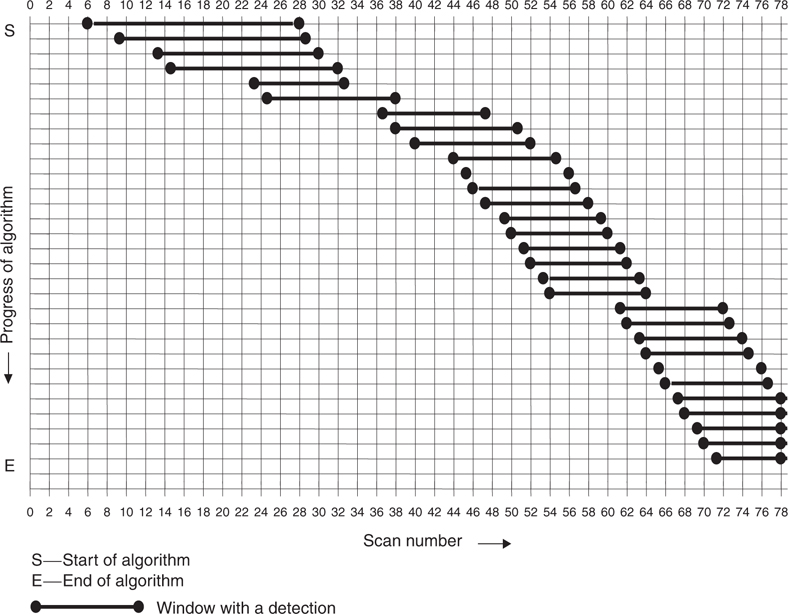
FIGURE 10.6
Progress of the algorithm showing windows with detections.

The next few detection windows produce similar target estimates. This is because a large number of scans repeat themselves in these windows.

After the initial detections, there is a “jump” in the scan number at which a detection is made. In addition, the estimates, particularly the velocity estimates, deteriorate. This could indicate that either the target has suddenly disappeared (became less visible) from the region of surveillance or the target made a maneuver.

From scan 44 onward, the algorithm stabilizes for several next windows. At scan 52, however, there is another jump in detection windows. This is also followed by a drop in the estimated target SNR, as explained above. This, however, indicates that the algorithm can adjust itself and restart after a target has become suddenly invisible. Recursive algorithms will diverge in this case.

From scan 54 onward, the algorithm stabilizes, as indicated by the estimates. Also, a detection is made for every increasing window because the target has come closer to the sensor and, thus, is more visible. This is noted by the sharp rise in the estimated target SNR after scan 54.

The above results provide an understanding of the target’s behavior. The results suggest that the Mirage F1 fighter jet appears late in the area of surveillance and moves toward the sensor. However, initially it remains quite invisible and possibly undergoes maneuvers. As it approaches the sensor, it becomes more and more visible and, thus, easier to detect.

10.5.4.2 Computational Load

The adaptive ML-PDA tracker took 442 s, including the time for data input/output, on a Pentium III processor running at 550 MHz to process the 78 scans of the Mirage F1 data. This translates into about 5.67 s/frame (or 5.67 s running time for one-second interval data), including input/output time. A more efficient implementation on a dedicated processor can easily make the algorithm real-time capable on a similar processor. Also, by parallelizing the initial grid search, which required more than 90% of the time, the adaptive ML-PDA estimator can be made even more efficient.

10.6 Summary

This chapter presented the use of the PDA technique for different tracking problems. Specifically, the PDA approach was used for parameter estimation as well as recursive state estimation. As an example of parameter estimation, track formation of a LO target using a nonlinear ML estimator in conjunction with the PDA technique with passive (sonar) measurements was presented. The use of the PDA technique in conjunction with the IMM estimator, resulting in the IMMPDAF, was presented as an example of recursive estimation on a radar-tracking problem in the presence of ECM. Also presented was an adaptive sliding-window PDA-based estimator that retains the advantages of the batch (parameter) estimator while being capable of tracking the motion of maneuvering targets. This was illustrated on an EO surveillance problem. These applications demonstrate the usefulness of the PDA approach for a wide variety of real tracking problems.

References

1. Bar-Shalom, Y. (Ed.), Multitarget-Multisensor Tracking: Advanced Applications, Vol. I, Artech House Inc., Dedham, MA, 1990. Reprinted by YBS Publishing, 1998.

2. Bar-Shalom, Y. (Ed.), Multitarget-Multisensor Tracking: Applications and Advances, Vol. II, Artech House Inc., Dedham, MA, 1992. Reprinted by YBS Publishing, 1998.

3. Bar-Shalom, Y. and Li, X. R., Multitarget-Multisensor Tracking: Principles and Techniques, YBS Publishing, Storrs, CT, 1995.

4. Blackman, S. S. and Popoli, R., Design and Analysis of Modern Tracking Systems, Artech House Inc., Dedham, MA, 1999.

5. Feo, M., Graziano, A., Miglioli, R., and Farina, A., IMMJPDA vs. MHT and Kalman filter with NN correlation: Performance comparison, IEE Proceedings on Radar, Sonar and Navigation (Part F), 144(2), 49–56, 1997.

6. Kirubarajan, T., Bar-Shalom, Y., Blair, W. D., and Watson, G. A., IMMPDA solution to benchmark for radar resource allocation and tracking in the presence of ECM, IEEE Transactions on Aerospace and Electronic Systems, 34(3), 1023–1036, 1998.

7. Lerro, D. and Bar-Shalom, Y., Interacting multiple model tracking with target amplitude feature, IEEE Transactions on Aerospace and Electronic Systems, AES-29(2), 494–509, 1993.

8. Blair, W. D., Watson, G. A., Kirubarajan, T., and Bar-Shalom, Y., Benchmark for radar resource allocation and tracking in the presence of ECM, IEEE Transactions on Aerospace and Electronic Systems, 34(3), 1015–1022, 1998.

9. Blackman, S. S., Dempster, R. J., Busch, M. T., and Popoli, R. F., IMM/MHT solution to radar benchmark tracking problem, IEEE Transactions on Aerospace and Electronic Systems, 35(2), 730–738, 1999.

10. Bar-Shalom, Y. and Li, X. R., Estimation and Tracking: Principles, Techniques and Software, Artech House Inc., Dedham, MA, 1993. Reprinted by YBS Publishing, 1998.

11. Jauffret, C. and Bar-Shalom, Y., Track formation with bearing and frequency measurements in clutter, IEEE Transactions on Aerospace and Electronic Systems, AES-26, 999–1010, 1990.

12. Kirubarajan, T., Wang, Y., and Bar-Shalom, Y., Passive ranging of a low observable ballistic missile in a gravitational field using a single sensor, Proceedings of the 2nd International Conference on Information Fusion, July 1999.

13. Sivananthan, S., Kirubarajan, T., and Bar-Shalom, Y., A radar power multiplier algorithm for acquisition of LO ballistic missiles using an ESA radar, Proceedings of the IEEE Aerospace Conference, March 1999.

14. Kirubarajan, T. and Bar-Shalom, Y., Target motion analysis in clutter for passive sonar using amplitude information, IEEE Transactions on Aerospace and Electronic Systems, 32(4), 1367–1384, 1996.

15. Nielsen, R. O., Sonar Signal Processing, Artech House Inc., Boston, MA, 1991.

16. Blair, W. D., Watson, G. A., Hoffman, S. A., and Gentry, G. L., Benchmark problem for beam pointing control of phased array radar against maneuvering targets, Proceedings of the American Control Conference, June 1995.

17. Blair, W. D. and Watson, G. A., IMM lgorithm for solution to benchmark problem for tracking maneuvering targets, Proceedings of SPIE Acquisition, Tracking and Pointing Conference, April 1994.

18. Blair, W. D., Watson, G. A., Hoffman, S. A., and Gentry, G. L., Benchmark problem for beam pointing control of phased array radar against maneuvering targets in the presence of ECM and false alarms, Proceedings of the American Control Conference, June 1995.

19. Yeddanapudi, M., Bar-Shalom, Y., and Pattipati, K. R., IMM estimation for multitarget-multisensor air traffic surveillance, Proceedings of IEEE, 85(1), 80–96, 1997.

20. Chummun, M. R., Kirubarajan, T., and Bar-Shalom, Y., An adaptive early-detection ML-PDA estimator for LO targets with EO sensors, Proceedings of SPIE Conference on Signal and Data Processing of Small Targets, 4048, 345–356, April 2000.

21. Press, W. H., Teukolsky, S. A., Vetterling, W. T., and Flannery, B. P., Numerical Recipes in C, Cambridge University Press, Cambridge, U.K., 1992.

22. Roszkowski, S. H., Common database for tracker comparison, Proceedings of SPIE Conference on Signal and Data Processing of Small Targets, 3373, 95–102, April 1998.

23. Lerro, D. and Bar-Shalom, Y., IR Target detection and clutter reduction using the interacting multiple model estimator, Proceedings of SPIE Conference on Signal and Data Processing of Small Targets, 3373, April 1998.

* When the running index is a time argument, a sequence exists; otherwise it is a set where the order is not relevant. The context should indicate which is the case.

* For other probabilistic models of the detection process, different SNR values correspond to the same P_D, P_FA pair. Compared to the Rician model receiver operating characteristic (ROC) curve, the Rayleigh model ROC curve requires a higher SNR for the same pair (P_D, P_FA), that is, the Rayleigh model considered here is pessimistic.

* The “uniform” factor corresponds to the worst case. In practice, σ_π and σ_γ are functions of the 3 dB bandwidth and the SNR.

† The commonly used SNR, designated here as SNR₁, is signal strength divided by the noise power in a 1 Hz bandwidth. SNR_c is signal strength divided by the noise power in a resolution cell. The relationship between them, for C_γ = 0.25 Hz is SNR_c = SNR₁–6 dB. SNR_c is believed to be the more meaningful SNR because it determines the ROC curve.

* The more recent IMM-MHT (as opposed to Kalman filter-based MHT) requires six to eight hypotheses.

* Assuming that this is a search pulse without (monopulse) split-beam processing, the angular errors are uniformly distributed in the beam.

..................Content has been hidden....................

You can't read the all page of ebook, please click here login for view all page.

Table of Contents for 10 Target Tracking Using Probabilistic Data Association-Based Techniques with Applications to Sonar, Radar, and EO Sensors

Create new playlist

Sign In

Sign Up

Table of Contents for
10 Target Tracking Using Probabilistic Data Association-Based Techniques with Applications to Sonar, Radar, and EO Sensors