
11
Introduction to the Combinatorics of Optimal and Approximate Data Association
Jeffrey K. Uhlmann
CONTENTS
11.3 Most Probable Assignments
11.5 Computational Considerations
11.6 Efficient Computation of Joint Assignment Matrix
11.7 Crude Permanent Approximations
11.8 Approximations Based on Permanent Inequalities
11.9 Comparisons of Different Approaches
11.10 Large-Scale Data Association
Appendix: Algorithm for Data Association Experiment
11.1 Introduction
Applying filtering algorithms to track the states of multiple targets first requires the correlation of the tracked objects with their corresponding sensor observations. A variety of probabilistic measures can be applied to each track estimate to determine independently how likely it is to have produced the current observation; however, such measures are useful only in practice for eliminating obviously infeasible candidates. Chapter 4 uses these measures to construct gates for efficiently reducing the number of feasible candidates to a number that can be accommodated within real-time computing constraints. Subsequent elimination of candidates can then be effected by measures that consider the joint relationships among the remaining track and report pairs.
After the gating step has been completed, a determination must be made concerning which feasible associations between observations and tracks are most likely to be correct. In a dense environment, however, resolving the ambiguities among various possible assignments of sensor reports to tracks may be impossible. The general approach proposed in the literature for handling such ambiguities is to maintain a set of hypothesized associations in the hope that some would be eliminated by future observations.19, 20 and 21 The key challenge is somehow to bound the overall computational cost by limiting the proliferation of pairs under consideration, which may increase in number at a geometric rate.
If n observations are made of n targets, one can evaluate an independent estimate of the probability that a given observation is associated with a given beacon. An independently computed probability, however, may be a poor indicator of how likely a particular observation is associated with a particular track because it does not consider the extent to which other observations may also be correlated with that item. More sophisticated methods generally require a massive batch calculation (i.e., they are a function of all n beacon estimates and O(n) observations of the beacons) where approximately one observation of each target is assumed.2,3 Beyond the fact that a real-time tracking system must process each sensor report as soon as it is obtained, the most informative joint measures of association scale exponentially with n and are, therefore, completely useless in practice.
This chapter examines some of the combinatorial issues associated with the batch data association problem arising in tracking and correlation applications. A procedure is developed that addresses a large class of data association problems involving the calculation of permanents of submatrices of the original association matrix. This procedure yields what is termed as the joint assignment matrix (JAM), which can be used to optimally rank associations for hypothesis selection. Because the computational cost of the permanent scales exponentially with the size of the matrix, improved algorithms are developed both for calculating the exact JAM and for generating approximations to it. Empirical results suggest that at least one of the approximations is suitable for real-time hypothesis generation in large-scale tracking and correlation applications. Novel theoretical results include an improved upper bound on the calculation of the JAM and new upper bound inequalities for the permanent of general nonnegative matrices. One of these inequalities is an improvement over the best previously known inequality.
11.2 Background
The batch data association problem2,4, 5, 6 and 7 can be defined as follows.
Given predictions about the states of n objects at a future time t, n measurements of that set of objects at time t, and a function to compute a probability of association between each prediction and measurement pair, calculate a new probability of association for a prediction and a measurement that is conditioned on the knowledge that the mapping from the set of predictions to the set of measurements is one-to-one.
For real-time applications, the data association problem is usually defined only in terms of estimates maintained at the current timestep of the filtering process. A more general problem can be defined that considers observations over a series of timesteps. Both problems are intractable, but the single-timestep variant appears to be more amenable to efficient approximation schemes.
As an example of the difference between these two measures of the probability of association, consider an indicator function that provides a binary measure of whether or not a given measurement is compatible with a given prediction. If the measure considers each prediction/measurement pair independently of all other predictions and measurements, then it could very well indicate that several measurements are feasible realizations of a single prediction. However, if one of the measurements has only that prediction as a feasible association, then from the constraint that the assignment is one-to-one, the measurement and the prediction must correspond to the same object. Furthermore, it can then be concluded, based on the same constraint, that the other measurements absolutely are not associated with that prediction. Successive eliminations of candidate pairs would hopefully yield a set of precisely n feasible candidates that must represent the correct assignment; however, this is rare in real-world applications. The example presented in Table 11.1 demonstrates the process.
TABLE 11.1
Assignment Example

The above-mentioned association problem arises in a number of practical tracking and surveillance applications. A typical example is the following: a surveillance aircraft flies over a region of ocean and reports the positions of various ships. Several hours later another aircraft repeats the mission. The problem then arises how to identify which reports in the second pass are associated with which reports from the earlier pass. The information available here includes known kinematic constraints (e.g., maximum speed) and the time difference between the various reports. If each ship is assumed to be traveling at a speed in the interval [vmin, vmax], then the indicator function can identify feasible pairs simply by determining which reports from the second pass fall within the radial interval [vmin∆t, vmax∆t] about reports from the first pass (see Figure 11.1). This problem is called track initiation2,4,3 because its solution provides a full position and velocity estimate, referred to as a track, which can then permit proper tracking.

FIGURE 11.1
The inner circle represents the possible positions of the ship if it travels at minimum speed, whereas the outer circle represents its possible positions at maximum speed.
After the tracking process has been initiated, the association problem arises again at the arrival of each batch of new reports. Thus, data association in this case is not a “one shot” problem; it is a problem of associating series of reports over a period of time to identify distinct trajectories. This means that attempting to remove ambiguity entirely at each step is not necessary; it is possible to retain a set of pairs in the hope that some would be eliminated at future steps. The maintenance of tentative tracks, referred to as hypotheses, is often termed as track splitting. Track splitting can be implemented in several ways, ranging from methods that simply add extra tracks to the track set with no logical structure to indicate which were formed from common reports, to methods that construct a complete “family tree” of tracks so that confirmation of a single leaf can lead to the pruning of large branches. No matter what the method is, the critical problem is to determine which pairs to keep and which to discard.
11.3 Most Probable Assignments
One way to deal with ambiguities arising in the joint analysis of the prior probabilities of association is to determine which of the a priori n! possible assignments is most probable. In this case, “most probable” means the assignment that maximizes the product of the prior probabilities of its component pairs. In other words, it is the assignment, σi, that maximizes
where aij is the matrix element giving the probability that track i is associated with report j. Unfortunately, this approach seems to require the evaluation and examination of n! products. There exists, however, a corpus of work on the closely related problem of optimal assignment (also known as maximum-weighted bipartite matching). The optimal assignment problem seeks the assignment that maximizes the sum of the values of its component pairs. In other words, it maximizes
This can be accomplished in O(n3) time.8 Thus, the solution to the maximum product problem can be obtained with an optimal assignment algorithm simply by using the logs of the prior probabilities, with the log of zero replaced with an appropriately large negative number. The optimal assignment approach eliminates ambiguity by assuming that the best assignment is always the correct assignment. Thus, it never maintains more than n tracks. The deficiency with this approach is that unless there are very few ambiguous pairs, many assignments will have almost the same probability. For example, if two proximate reports are almost equally correlated with each of two tracks, then swapping their indices in the optimal assignment will generate a new but only slightly less probable assignment. In fact, in most nontrivial applications, the best assignment has a very low probability of being correct.
The optimal assignment method can be viewed as the best choice of track–report pairs if the criterion is to maximize the probability of having all the pairs correct. Another reasonable optimality criterion would seek the set of n pairs that maximizes the expected number of pairs that are correct. To illustrate the difference between these criteria, consider the case in which two proximate reports are almost equally correlated with two tracks, and no others. The optimal assignment criterion would demand that the two reports be assigned to distinct tracks, whereas the other criterion would permit all four pairs to be kept as part of the n selected pairs. With all four possible pairs retained, the second criterion ensures that at least two are correct. The two pairs selected by the optimal assignment criterion, however, have almost a .5 probability of both being incorrect.
11.4 Optimal Approach
A strategy for generating multiple hypotheses within the context of the optimal assignment approach is to identify the k best assignments and take the union of their respective pairings.5,9,10 The assumption is that pairs in the most likely assignments are most likely to be correct. Intuition also would suggest that a pair common to all the k best assignments stands a far better chance of being correct than its prior probability of association might indicate. Generalizing this intuition leads to the exact characterization of the probabilities of association under the assignment constraint. Specifically, the probability that report Ri is associated with track Tj is simply the sum of the probabilities of all the assignments containing the pair, normalized by the sum of the probabilities of all assignments:5
For example, suppose the following matrix is given containing the prior probabilities of association for two tracks with two reports:
Given the assignment constraint, the correct pair of associations must be either (T1, R1) and (T2, R2), or (T1, R2) and (T2, R1). To assess the joint probabilities of association, Equation 11.3 must be applied to each entry of the matrix to obtain:
Notice that the resulting matrix is doubly stochastic (i.e., it has rows and columns all of which sum to unity), as one would expect. (The numbers in the matrix in Equation 11.5 have been rounded, but still sum appropriately. One can verify that the true values do as well.) Notice also that the diagonal elements are equal. This is the case for any 2 × 2 matrix because elements of either diagonal can only occur jointly in an assignment; therefore, one element of a diagonal cannot be more or less likely than the other. The matrix of probabilities generated from the assignment constraint is JAM.
Now consider the following matrix:
which, given the assignment constraint, leads to the following:
This demonstrates how significant the difference can be between the prior and the joint probabilities. In particular, the pair (T1, R1) has a prior probability of .9, which is extremely high. Considered jointly with the other measurements, however, its probability drops to only .31.
A more extreme example is the following:
which leads to
where the fact that T2 cannot be associated with R2 implies that there is only one feasible assignment. Examples like this show why a “greedy” selection of hypotheses based only on the independently assessed prior probabilities of association can lead to highly suboptimal results.
The examples that have been presented here have considered only the ideal case where the actual number of targets is known and the number of tracks and reports equals that number. However, the association matrix can easily be augmented* to include rows and columns to account for the cases in which some reports are spurious and some targets are not detected. Specifically, a given track can have a probability of being associated with each report as well as a probability of not being associated with any of them. Similarly, a given report has a probability of association with each of the tracks and a probability that it is a false alarm not associated with any target. Sometimes a report that is not associated with any tracks signifies a newly detected target. If the actual number of targets is not known, a combined probability of false alarm and probability of new target must be used. Estimates of probabilities of detection, probabilities of false alarms, and probabilities of new detections are difficult to determine because of complex dependencies on the type of sensor used, the environment, the density of targets, and a multitude of other factors whose effects are almost never known. In practice, such probabilities are often lumped together into one tunable parameter (e.g., a “fiddle factor”).
11.5 Computational Considerations
A closer examination of Equation 11.3 reveals that the normalizing factor is a quantity that resembles the determinant of the matrix, but without the alternating ±1 factors. In fact, the determinant of a matrix is just the sum of products over all even permutations minus the sum of products over all odd permutations. The normalizing quantity of Equation 11.3, however, is the sum of products over all permutations. This latter quantity is called the permanent6,11,1 of a matrix, and it is often defined as follows:
where the summation extends over all permutations Q of the integers 1, 2, …, n. The Laplace expansion of the determinant also applies for the permanent:
where is the submatrix obtained by removing row i and column j. This formulation provides a straightforward mechanism for evaluating the permanent, but it is not efficient. As in the case of the determinant, expanding by Laplacians requires O(n … n!) computations. The unfortunate fact about the permanent is that although the determinant can be evaluated by other means in O(n3) time, effort exponential in n seems to be necessary to evaluate the permanent.12
If Equation 11.3 were evaluated without the normalizing coefficient for every element of the matrix, determining the normalizing quantity by simply computing the sum of any row or column would seem possible as the result must be doubly stochastic. In fact, this is the case. Unfortunately, Equation 11.3 can be rewritten, using Equation 11.11, as
where the evaluation of permanents seems unavoidable. Knowing that such evaluations are intractable, the question then is how to deal with computational issues.
The most efficient method for evaluating the permanent is attributable to Ryser.6 Let A be an n × n matrix, let Ar denote a submatrix of A obtained by deleting r columns, let ∏(Ar) denote the product of the row sums of Ar, and let ∑∏(Ar) denote the sum of the products ∏(Ar) taken over all possible Ar. Then,
This formulation involves only O(2n), rather than O(n!), products. This may not seem like a significant improvement, but for n in the range of 10–15, the reduction in compute time is from hours to minutes on a typical workstation. For n greater than 35, however, scaling effects thwart any attempt at evaluating the permanent. Thus, the goal must be to reduce the coefficients as much as possible to permit the optimal solution for small matrices in real time, and to develop approximation schemes for handling large matrices in real time.
11.6 Efficient Computation of Joint Assignment Matrix
Equation 11.13 is known to permit the permanent of a matrix to be computed in O(n2 … 2n) time. From Equation 11.12, then, one can conclude that the JAM is computable in O(n4 … 2n) time (i.e., the amount of time required to compute the permanent of Aij for each of the n2 elements aij). However, this bound can be improved by showing that the JAM can be computed in O(n3 … 2n) time, and that the time can be further reduced to O(n2 … 2n).
First, the permanent of a general matrix can be computed in O(n … 2n) time. This is accomplished by eliminating the most computationally expensive step in direct implementations of Ryser’s method—the O(n2) calculation of the row sums at each of the 2n iterations. Specifically, each term of Ryser’s expression of the permanent is just a product of the row sums with one of the 2n subsets of columns removed. A direct implementation therefore requires the summation of the elements of each row that are not in one of the removed columns. Thus, O(n) elements are summed for each of the n rows at a total cost of O(n2) arithmetic operations per term. To reduce the cost required to update the row sums, Nijenhuis and Wilf showed that the terms in Ryser’s expression can be ordered so that only one column is changed from one term to the next.13 At each step the algorithm updates the row sums by either adding or subtracting the column element corresponding to the change. Thus, the total update time is only O(n). This change improves the computational complexity from O(n2 … 2n) to O(n … 2n).
The above-mentioned algorithm for evaluating the permanent of a matrix in O(n … 2n) time can be adapted for the case in which a row and a column of a matrix are assumed removed. This permits the evaluation of the permanents of the submatrices associated with each of the n2 elements, as required by Equation 11.12, to calculate the JAM in O(n3 … 2n) time. This is an improvement over the O(n4 … 2n) scaling obtained by the direct application of Ryser’s formula (Equation 11.13) to calculate the permanent of each submatrix. The scaling can, however, be reduced even further. Specifically, note that the permanent of the submatrix associated with element aij is the sum of all ((n − 1)2(n−1))/(n − 1) terms in Ryser’s formula that do not involve row i or column j. In other words, one can eliminate a factor of (n − 1) by factoring the products of the (n − 1) row sums common to the submatrix permanents of each element in the same row. This factorization leads to an optimal JAM algorithm with complexity O(n2 … 2n).14
An optimized version of this algorithm can permit the evaluation of 12 × 12 joint assignment matrices in well under a second. Because the algorithm is highly parallelizable—the O(2n) iterative steps can be divided into k subproblems for simultaneous processing on k processors—solutions to problems of size n in the range of 20–25 should be computable in real time with O(n2) processors. Although not practical, the quantities computed at each iteration could also be computed in parallel on n … 2n processors to achieve an O(n2) sequential scaling. This might permit the real-time solution of somewhat larger problems but at an exorbitant cost. Thus, the processing of n … n matrices, for n > 25, will require approximations.
Figure 11.2 provides actual empirical results (on a ca. 1994 workstation) showing that the algorithm is suitable for real-time applications for n < 10, and it is practical for offline applications for n as large as 25. The overall scaling has terms of n22n and 2n, but the test results and the algorithm itself clearly demonstrate that the coefficient on the n22n term is small relative to the 2n term.

FIGURE 11.2
Tests of the new joint assignment matrix algorithm reveal the expected exponentially scaling computation time.
11.7 Crude Permanent Approximations
In the late 1980s, several researchers identified the importance of determining the number of feasible assignments in sparse association matrices arising in tracking applications. In this section, a recently developed approach for approximating the JAM via permanent inequalities is described, which yields surprisingly good results within time roughly proportional to the number of feasible track–report pairs.
Equation 11.12 shows that an approximation to the permanent would lead to a direct approximation of Equation 11.3. Unfortunately, research into approximating the permanent has emphasized the case in which the association matrix A has only 0–1 entries.15 Moreover, the methods for approximating the permanent, even in this restricted case, still scale exponentially for reasonable estimates.15, 16 and 17 Even “unreasonable” estimates for the general permanent, however, may be sufficient to produce a reasonable estimate of a conditional probability matrix. This is possible because the solution matrix has additional structure that may permit the filtering of noise from poorly estimated permanents. The fact that the resulting matrix should be doubly stochastic, for example, suggests that the normalization of the rows or columns (i.e., dividing each row or column by the sum of its elements) should improve the estimate.
One of the most important properties of permanents relating to the doubly stochastic property of the JAM is the following: Multiplying a row or column by a scalar c has the effect of multiplying the permanent of the matrix by the same factor.1,6,11 This fact verifies that the multiplication of a row or column by some c also multiplies the permanent of any submatrix by c. This implies that the multiplication of any combination of rows or columns of a matrix by any values (other than zero) has no effect on the JAM. This is because the factors applied to the various rows and columns cancel in the ratio of permanents in Equation 11.12. Therefore, the rows and columns of a matrix can be normalized in any manner before attempting to approximate the JAM.
To see why a conditioning step could help, consider a 3 × 3 matrix with all elements equal to 1. If row 1 and column 1 are multiplied by 2, then the following matrix is obtained:
where the effect of the scaling of the first row and column has been undone.* This kind of preconditioning could be expected to improve the reliability of an estimator. For example, it seems to provide more reliable information for the greedy selection of hypotheses. This iterative process could also be useful for the postconditioning of an approximate JAM (e.g., to ensure that the estimate is doubly stochastic). Remember that its use for preconditioning is permissible because it does nothing more than scale the rows and columns during each iteration, which does not affect the obtained JAM. The process can be repeated for O(n) iterations,† involves O(n2) arithmetic operations per iteration, and thus scales as O(n3). In absolute terms, the computations take about the same amount of compute time as required to perform an n × n matrix multiply.
11.8 Approximations Based on Permanent Inequalities
The possibility has been discussed of using crude estimators of the permanent, combined with the knowledge about the structure of the JAM, to obtain better approximations. Along these lines, four upper bound inequalities, ε1 – ε4, for the permanent are examined for use as crude estimators. The first inequality, ε1, is a well-known result:
where ri is the sum of the elements in row i. This inequality holds for nonnegative matrices because it sums over all products that do not contain more than one element from the same row. In other words, it sums over a set larger than that of the actual permanent because it includes products with more than one element from the same column. For example, the above-mentioned inequality applied to a 2 × 2 matrix would give a11a21 + a11a22 + a12a21 + a12a22, rather than the sum over one-to-one matchings a11a22 + a12a21. In fact, the product of the row sums is the first term in Ryser’s equation. This suggests that the evaluation of the first k terms should yield a better approximation. Unfortunately, the required computation scales exponentially in the number of evaluated terms, thus making only the first two or three terms practical for approximation purposes. All the inequalities in this section are based on the first term of Ryser’s equation applied to a specially conditioned matrix. They can all, therefore, be improved by the use of additional terms, noting that an odd number of terms yields an upper bound, whereas an even number yields a lower bound.
This inequality also can be applied to the columns to achieve a potentially better upper bound. This would sum over products that do not contain more than one element from the same column. Thus, the following bound can be placed on the permanent:1,6,11
Although taking the minimum of the product of the row sums and the product of the column sums tends to yield a better bound on the permanent, there is no indication that it is better than always computing the bound with respect to the rows. This is because the goal is to estimate the permanent of a submatrix for every element of the matrix, as required by Equation 11.12, to generate an estimate of the JAM. If all of the estimates are of the same “quality” (i.e., are all too large by approximately the same factor), then some amount of postconditioning could yield good results. If the estimates vary considerably in their quality, however, postconditioning might not provide significant improvement.
The second inequality considered, ε2, is the Jurkat–Ryser upper bound:11,18 Given a nonnegative n × n matrix A = [aij] with row sums r1, r2, …, rn and column sums c1, c2, …, cn, where the row and column sums are indeed so that rk ≤ rk+1 and ck ≤ ck+1 for all k, then:
For cases in which there is at least one k, such that rk ≠ ck, this upper bound is less than that obtained from the product of row or column sums. This has been the best of all known upper bounds since it was discovered in 1966. The next two inequalities, ε3 and ε4, are the new results.14
ε3 is defined as
This inequality is obtained by normalizing the columns, computing the product of the row sums of the resulting matrix, and then multiplying that product by the product of the original column sums. In other words,
Note that the first summation is just the row sums after the columns have been normalized.
This new inequality is interesting because it seems to be the first general upper bound to be discovered, which is, in some cases, superior to Jurkat–Ryser. For example, consider the following matrix:
Jurkat–Ryser (ε2) yields an upper bound of 15, whereas the estimator ε3 yields a bound of 13.9. Although ε3 is not generally superior, it is considered for the same reasons as the estimator ε1.
The fourth inequality considered, ε4, is obtained from ε3 via ε2:
The inequality is derived by first normalizing the columns. Then applying Jurkat–Ryser with all column sums equal to unity yields the following:
where the first summation simply represents the row sums after the columns have been normalized.
Similar to ε1 and ε3, this inequality can be applied with respect to the rows or columns—whichever yields the better bound. In the case of ε4, this is critical because one case usually provides a bound that is smaller than the other and is smaller than that obtained from Jurkat–Ryser.
In the example matrix (Equation 11.22), the ε4 inequality yields an upper bound of 11, an improvement over the other three estimates. Small-scale tests of the four inequalities on matrices of uniform deviates suggest that ε3 almost always provides better bounds than ε1, ε2 almost always provides better bounds than ε3, and ε4 virtually always (more than 99% of the time) produces superior bounds to the other three inequalities. In addition to producing relatively tighter upper bound estimates in this restricted case, inequality ε4 should be more versatile analytically than Jurkat–Ryser because it does not involve a reindexing of the rows and columns.
11.9 Comparisons of Different Approaches
Several of the JAM approximation methods described in this chapter have been compared on matrices containing
Uniformly and independently generated association probabilities
Independently generated binary (i.e., 0–1) indicators of feasible association
Probabilities of association between two three-dimensional (3D) sets of correlated objects
The third group of matrices was generated from n tracks with uniformly distributed means and equal covariances by sampling the Gaussian defined by each track covariance to generate n reports. A probability of association was then calculated for each track–report pair.
The first two classes of matrices are examined to evaluate the generality of the various methods. These matrices have no special structure to be exploited. Matrices from the third class, however, contain structure typical of association matrices arising in tracking and correlation applications. Performance on these matrices should be indicative of performance in real-world data association problems, whereas performance in the first two classes should reveal the general robustness of the approximation schemes.
The approximation methods considered are the following:
ε1, the simplest of the general upper bound inequalities on the permanent. Two variants are considered
The upper bound taken with respect to the rows
The upper bound taken with respect to the rows or columns, whichever is less Scaling: O(n3)
ε2, the Jurkat–Ryser inequality
Scaling: O(n3 log n)
ε3 with two variants:
The upper bound taken with respect to the rows
The upper bound taken with respect to the rows or columns, whichever is less Scaling: O(n3) (see the appendix)
ε4 with two variants
The upper bound taken with respect to the rows
The upper bound taken with respect to the rows or columns, whichever is less Scaling: O(n3)
Iterative renormalization alone
Scaling: O(n3)
The standard greedy method2 that assumes the prior association probabilities are accurate (i.e., performs no processing of the association matrix)
Scaling: O(n2 log n)
The one-sided normalization method that normalizes only the rows (or columns) of the association matrix
Scaling: O(n2 log n)
The four ε estimators include the O(n3) cost of pre- and postprocessing via iterative renormalization.
The quality of hypotheses generated by the greedy method O(n2 log n) is also compared to those generated optimally via the JAM. The extent to which the greedy method is improved by first normalizing the rows (or columns) of the association matrix is also examined. The latter method is relevant for real-time data association applications in which the set of reports (or tracks) cannot be processed in batch.
Tables 11.2, 11.3 and 11.4 give the results of the various schemes when applied to different classes of n × n association matrices. The n best associations for each scheme are evaluated via the true JAM to determine the expected number of correct associations. The ratio of the expected number of correct associations for each approximation method and the optimal method yields the percentages in Table 11.2.* For example, an entry of 50% implies that the expected number of correct associations is half of what would be obtained from the JAM.
Table 11.2 provides a comparison of the schemes on matrices of size 20 × 20. Matrices of this size are near the limit of practical computability. For example, the JAM computations for a 35 × 35 matrix would demand more than a hundred years of nonstop computing on current high-speed workstations.
TABLE 11.2
Results of Tests of Several Joint Assignment Matrix Approximation Methods on 20 × 20 Association Matrices (% Optimal)

TABLE 11.3
Results of Tests of the Joint Assignment Matrix Approximation on Variously Sized Association Matrices Generated from Uniform Random Deviates

The most interesting information that has been provided by Table 11.2 is that the inequality-based schemes are all more than 99% of optimal, with the approximation based on the Jurkat–Ryser inequality performing worst. The ε3 and ε4 methods performed best and always yielded identical results on the doubly stochastic matrices obtained by preprocessing. Preprocessing also improved the greedy scheme by 10–20%. Tables 11.3 and 11.4 show the effect of matrix size on each of the methods.
In almost all cases, the inequality-based approximations seemed to improve with matrix size. The obvious exception is the case of 5 × 5 0−1 matrices—the approximations are perfect because there tends to be only one feasible assignment for randomly generated 5 × 5 0−1 matrices. Surprisingly, the one-sided normalization approach is 80–90% optimal, yet scales as O(p log p), where p is the number of feasible pairings.
The one-sided approach is the only practical choice for large-scale applications that do not permit batch processing of sensor reports because the other approaches require the generation of the (preferably sparse) assignment matrix. The one-sided normalization approach requires only the set of tracks with which it gates (i.e., one row of the assignment matrix). Therefore, it permits the sequential processing of measurements. Of the methods compared here, it is the only one that satisfies online constraints in which each observation must be processed at the time it is received.
TABLE 11.4
Results of Tests of the Joint Assignment Matrix Approximation on Variously Sized Association Matrices Generated from Uniform 0–1 Random Deviates

To summarize, the JAM approximation schemes based on the new permanent inequalities appear to yield near-optimal results. An examination of the matrices produced by these methods reveals a standard deviation of less than 3 × 10⁻⁵ from the optimal JAM computed via permanents. The comparison of expected numbers of correct assignments given in the Tables 11.2, 11.3 and 11.4, however, is the most revealing in terms of applications to multiple-target tracking. Specifically, the recursive formulation of the tracking process leads to highly nonlinear dependencies on the quality of the hypothesis generation scheme. In a dense tracking environment, a deviation of less than 1% in the expected number of correct associations can make the difference between convergence and divergence of the overall process. The next section considers applications to large-scale problems.
11.10 Large-Scale Data Association
This section examines the performance of the one-sided normalization approach. The evidence provided in the Section 11.9 indicates that the estimator ε3 yields probabilities of association conditioned on the assignment constraint that are very near optimal. Therefore, ε3 can be used as a baseline of comparison for the one-sided estimator for problems that are too large to apply the optimal approach. The results in the previous section demonstrate that the one-sided approach yields relatively poor estimates when compared to the optimal and near-optimal methods. However, because the latter approaches cannot be applied online to process each observation as it arrives, the one-sided approach is the only feasible alternative. The goal, therefore, is to demonstrate only that its estimates do not diminish in quality as the size of the problem increases. This is necessary to ensure that a system that is tuned and tested on problems of a given size behaves predictably when applied to larger problems.
In the best-case limit, as the amount of ambiguity goes to zero, any reasonable approach to data association should perform acceptably. In the worst-case limit, as all probabilities converge to the same value, no approach can perform any better than a simple random selection of hypotheses. The worst-case situation in which information can be exploited is when the probabilities of association appear to be uncorrelated random deviates. In such a case, only higher-order estimation of the joint probabilities of association can provide useful discriminating information. In Table 11.5 is an example of an association matrix that was generated from a uniform random number generator. This example matrix was chosen from among the 10 that were generated because it produced the most illustrative JAM. The uniform deviate entries have been divided by n so that they are of magnitude comparable to that of actual association probabilities.
TABLE 11.5
Example of an Association Matrix Generated from a Uniform Random Number Generator
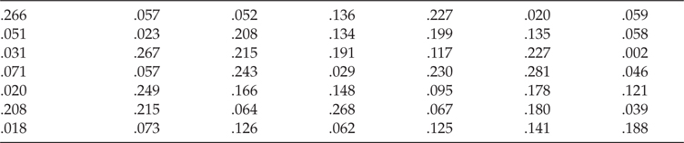
TABLE 11.6
True Probabilities of Association Conditioned on the Assignment Constraint

Applying the optimal JAM algorithm yields the true probabilities of association conditioned on the assignment constraint, as shown in Table 11.6.
A cursory examination of the differences between corresponding entries in the two matrices demonstrates that a significant amount of information has been extracted by considering higher-order correlations. For example, the last entries in the first two rows of the association matrix are .059 and .058—differing by less than 2%—yet their respective JAM estimates are .077 and .109, a difference of almost 30%. Remarkably, despite the fact that the entries in the first matrix have been generated from uniform deviates, the first entry in the first row and the last entry in the last row of the resulting JAM represent hypotheses that each have a better than 50% chance of being correct.
To determine whether the performance of the one-sided hypothesis selection approach suffers as the problem size is increased, its hypotheses have been compared with those of estimator ε3 on n × n, for n in the range of 10–100, association matrices generated from uniform random deviates. Figure 11.3 shows that the number of correct associations for the one-sided approach seems to approach the same number as ε3 as n increases. This may be somewhat misleading, however, because the expected number of correct associations out of n hypotheses selected from n × n possible candidates would tend to decrease as n increases. More specifically, the ratio of correct associations to number of hypotheses (proportional to n) would tend to zero for all methods if the prior probabilities of association are generated at random.
A better measure of performance is how many hypotheses are necessary for a given method to ensure that a fixed number are expected to be correct. This can be determined from the JAM by summing its entries corresponding to a set of hypotheses. Because each entry contains the expectation that a particular track–report pair corresponds to the same object, the sum of the entries gives the expected number of correct assignments. To apply this measure, it is necessary to fix a number of hypotheses that must be correct, independent of n, and determine the ratio of the number of hypotheses required for the one-sided approach to that required by ε3. Figure 11.4 also demonstrates that the one-sided method seems to approach the same performance as ε3 as n increases in a highly ambiguous environment. In conclusion, the performance of the one-sided approach scales robustly even in highly ambiguous environments.

FIGURE 11.3
The performance of the one-sided approach relative to ε3 improves with increasing N. This is somewhat misleading, however, because the expected number of correct assignments goes to zero in the limit N → ∞ for both approaches.

FIGURE 11.4
This test plots the number of hypotheses required by the one-sided approach to achieve some fixed expected number of correct assignments. Again, it appears that the one-sided approach performs comparably to ε3 as N increases.
The good performance of the one-sided approach—which superficially appears to be little more than a crude heuristic—is rather surprising given the amount of information it fails to exploit from the association matrix. In particular, it uses information only from the rows (or columns) taken independently, thus making no use of information provided by the columns (or rows). Because the tests described in the previous text have all rows and columns of the association matrix scaled randomly, but uniformly, the worst-case performance of the one-sided approach may not have been seen. In tests in which the columns have been independently scaled by vastly different values, results generated from the one-sided approach show little improvement over those of the greedy method. (The performances of the optimal and near-optimal methods, of course, are not affected.) In practice, a system in which all probabilities are scaled by the same value (e.g., as a result of using a single sensor) should not be affected by this limitation of the one-sided approach. In multisensor applications, however, association probabilities must be generated consistently. If a particular sensor is not modeled properly, and its observations produce track–report pairs with consistently low or high probabilities of association, then the hypotheses generated from these pairs by the one-sided approach would be ranked consistently low or high.
11.11 Generalizations
The combinatorial analysis of the assignment problem in Sections 11.9 and 11.10 has considered only the case of a single “snapshot” of sensor observations. In actual tracking applications, however, the goal is to establish tracks from a sequence of snapshots. Mathematically, the definition of a permanent can be easily generalized to apply not only to assignment matrices but also to tensor extensions. Specifically, the generalized permanent sums over all assignments of observations at timestep k, for each possible assignment of observations at timestep k – 1, continuing recursively down to the base case of all possible assignments of the first batch of observations to the initial set of tracks. (This multidimensional assignment problem is described more fully in Chapter 13.) Although generalizing the crude permanent approximations for application to the multidimensional assignment problem is straightforward, the computation time scales geometrically with exponent k. This is vastly better than the super-exponential scaling required for the optimal approach, but it is not practical for large values of n and k unless the gating process yields a very sparse association matrix (see Chapter 4).
11.12 Conclusions
This chapter has discussed some of the combinatorial issues arising in the batch data association problem. It has described the optimal solution for a large class of data association problems involving the calculation of permanents of submatrices of the original association matrix. This procedure yields the JAM, which can be used to optimally rank associations for hypothesis selection. Because the computational cost of the permanent scales exponentially in the size of the matrix, improved algorithms have been developed both for calculating the exact JAM and for generating approximations to it. Empirical results suggest that the approximations are suitable for hypothesis generation in large-scale tracking and correlation applications. New theoretical results include an improved upper bound on the calculation of the JAM and new upper bound inequalities, ε3 and ε4, for the permanent of general nonnegative matrices.
The principal conclusion that can be drawn from this chapter is that the ambiguities introduced by a dense environment are extremely difficult and computationally expensive to resolve. Although this chapter has examined the most general possible case in which tracking has to be performed in an environment that is dense with indistinct (other than position) targets, there is little doubt that the constraints imposed by most real-world applications would necessitate some sacrifice of this generality.
Acknowledgments
The author gratefully acknowledges support from the University of Oxford, UK, and the Naval Research Laboratory, Washington, DC.
Appendix: Algorithm for Data Association Experiment
The following algorithm demonstrates how O(n3) scaling can be obtained for approximating the JAM of an n × n association matrix using inequality ε3. A straightforward implementation that scales as O(n4) can be obtained easily; the key to removing a factor of n comes from the fact that from a precomputed product of row sums, rprod, the product of all row sums excluding row i is just rprod divided by row sum i. In other words, performing an O(n) step of explicitly computing the product of all row sums except row i is not necessary. Some care must be taken to accommodate row sums that are zero, but the following pseudocode shows that there is little extra overhead incurred by the more efficient implementation. Similar techniques lead to the advertised scaling for the other inequality approaches. (Note, however, that sums of logarithms should be used in place of explicit products to ensure numerical stability in actual implementations.)
E3r(M, P, n)
r and c are vectors of length n corresponding to the row and column sums, respectively. rn is a vector of length n of normalized row sums.
for i = 1 to n: ri ← ci ← 0.0
Apply iterative renormalization to M
for i = 1 to n:
for j = 1 to n:
ri ← ri + Mij
ci ← ci + Mij
end
end
for i = 1 to n:
for l = 1 to n:
rnl ← 0.0
for k = 1 to n, if (ck – Mik) > 0.0
then rnl ← rnl + Mik/(ck – Mik)
end
for j = 1 to n:
nprod = 1.0
for k = 1 to n, if k ≠ j
then nprod ← nprod* (ck – Mik)
rprod ← cprod ← 1.0
for k = 1 to n, if k ≠ 1
if (cj – Mij) > 0.0
then rprod ← rprod* (rnk – Mkj)/(cj – Mij)
else rprod ← rprod* rnk
end
rprod ← rprod* nprod
Pij ← Mij* rprod
end
end
Apply iterative renormalization to P
end.
References
1. Minc, H., Permanents, Encyclopedia of Mathematics and its Applications, 4th edition, Vol. 6, Part F, Addison-Wesley, New York, NY, 1978.
2. Blackman, S., Multiple-Target Tracing with Radar Applications, Artech House, Dedham, MA, 1986.
3. Blackman, S. and Popoli, R., Design and Analysis of Modern Tracking Systems, Artech House, Norwood, MA, 1999.
4. Bar-Shalom, Y. and Fortmann, T.E., Tracking and Data Association, Academic Press, New York, NY, 1988.
5. Collins, J.B. and Uhlmann, J.K., Efficient gating in data association for multivariate Gaussian distributions, IEEE Transactions on Aerospace and Electronic Systems, 28(3), 909–916, 1990.
6. Ryser, H.J., Combinatorial Mathematics, 14, Carus Mathematical Monograph Series, Mathematical Association of America, 1963.
7. Uhlmann, J.K., Algorithms for multiple-target tracking, American Scientist, 80(2), 128–141, 1992.
8. Papadimitrious, C.H. and Steiglitz, K., Combinatorial Optimization Algorithms and Complexity, Prentice Hall, Englewood Cliffs, NJ, 1982.
9. Cox, I.J. and Miller, M.L., On finding ranked assignments with application to multitarget tracking and motion correspondence, IEEE Transactions on Aerospace and Electronic Systems, 31, 486–489, 1995.
10. Nagarajan, V., Chidambara, M.R., and Sharma, R.M., New approach to improved detection and tracking in track-while-scan radars, Part 2: Detection, track initiation, and association, IEEE Proceedings, 134(1), 89–92, 1987.
11. Brualdi, R.A. and Ryser, H.J., Combinatorial Matrix Theory, Cambridge University Press, Cambridge, UK, 1992.
12. Valiant, L.G., The complexity of computing the permanent, Theoretical Computer Science, 8, 189–201, 1979.
13. Nijenhuis, A. and Wilf, H.S., Combinatorial Algorithms, 2nd edition, Academic Press, New York, NY, 1978.
14. Uhlmann, J.K., Dynamic Localization and Map Building: New Theoretical Foundations, PhD thesis, University of Oxford, 1995.
15. Karmarkar, N. et al., A Monte Carlo algorithm for estimating the permanent, SIAM Journal on Computing, 22(2), 284–293, 1993.
16. Jerrum, M. and Vazirani, U., A Mildly Exponential Approximation Algorithm for the Permanent, Technical Report, Department of Computer Science, University of Edinburgh, Scotland, 1991. ECS-LFCS-91–179.
17. Jerrum, M. and Sinclair, A., Approximating the permanent, SIAM Journal on Computing, 18(6), 1149–1178, 1989.
18. Jurkat, W.B. and Ryser, H.J., Matrix factorizations of determinants and permanents, Journal of Algebra, 3, 1–27, 1966.
19. Reid, D.B., An algorithm for tracking multiple targets, IEEE Transactions on Automatic Control, AC-24(6), 843–854, 1979.
20. Cox, I.J. and Leonard, J.J., Modeling a dynamic environment using a Bayesian multiple hypothesis approach, Artificial Intelligence, 66(2), 311–344, 1994.
21. Bar-Shalom, Y. and Li, X.R., Multitarget-Multisensor Tracking: Principles and Techniques, YBS Press, Storrs, CT, 1995.
* Remember the use of an association “matrix” is purely for notational convenience. In large applications, such a matrix would not be generated in its entirety; rather, a sparse graph representation would be created by identifying and evaluating only those entries with probabilities above a given threshold.
* A physical interpretation of the original matrix in sensing applications is that each row and column corresponds to a set of measurements, which is scaled by some factor due to different sensor calibrations or models.
† This iterative algorithm for producing a doubly stochastic matrix is best known in the literature as the Sinkhorn iteration, and many of its properties have been extensively analyzed.
* The percentages are averages over enough trials to provide an accuracy of at least five decimal places in all cases except tests involving 5 × 5 0–1 matrices. The battery of tests for the 5 × 5 0–1 matrices produced some instances in which no assignments existed. The undefined results for these cases were not included in the averages, so the precision may be slightly less.