12 Bayesian Approach to Multiple-Target Tracking

This chapter views the multiple-target tracking problem as a Bayesian inference problem and highlights the benefits of this approach. The goal of this chapter is to provide the reader with some insights and perhaps a new view of the multiple-target tracking. It is not designed to provide the reader with a set of algorithms for multiple-target tracking.

The chapter begins with a Bayesian formulation of the single-target tracking problem and then extends this formulation to multiple targets. It then discusses some of the interesting consequences of this formulation, including

A mathematical formulation of the multiple-target tracking problem with a minimum of complications and formalisms
The emergence of likelihood functions as a generalization of the notion of contact and as the basic currency for valuing and combining information from disparate sensors
A general Bayesian formula for calculating association probabilities
A method, called unified tracking, for performing multiple-target tracking when the notions of contact and association are not meaningful
A delineation of the relationship between multiple-hypothesis tracking (MHT) and unified tracking
A Bayesian track-before-detect methodology called likelihood ratio detection and tracking

12.1.1 Definition of Bayesian Approach

To appreciate the discussion in this chapter, the reader must first understand the concept of Bayesian tracking. For a tracking system to be considered Bayesian, it must have the following characteristics:

Prior distribution. There must be a prior distribution on the state of the targets. If the targets are moving, the prior distribution must include a probabilistic description of the motion characteristics of the targets. Usually the prior is given in terms of a stochastic process for the motion of the targets.
Likelihood functions. The information in sensor measurements, observations, or contacts must be characterized by likelihood functions.
Posterior distribution. The basic output of a Bayesian tracker is a posterior probability distribution on the (joint) state of the target(s). The posterior at time t is computed by combining the motion-updated prior at time t with the likelihood function for the observation(s) received at time t.

These are the basics: prior, likelihood functions, and posterior. If these are not present, the tracker is not Bayesian. The recursions given in this chapter for performing Bayesian tracking are all recipes for calculating priors, likelihood functions, and posteriors.

12.1.2 Relationship to Kalman Filtering

Kalman filtering resulted from viewing tracking as a least-squares problem and finding a recursive method of solving that problem. One can think of many standard tracking solutions as methods for minimizing mean squared errors. Chapters 1, 2 and 3 of Ref. 1 give an excellent discussion on tracking from this point of view. One can also view Kalman filtering as Bayesian tracking. To do this, one starts with a prior that is Gaussian in the appropriate state space with a very large covariance matrix. Contacts are measurements that are linear functions of the target state with Gaussian measurement errors. These are interpreted as Gaussian likelihood functions and combined with motion-updated priors to produce posterior distributions on target state. Because the priors are Gaussian and the likelihood functions are Gaussian, the posteriors are also Gaussian. When doing the algebra, one finds that the mean and covariance of the posterior Gaussian are identical to the mean and covariance of the least-squares solution produced by the Kalman filter. The difference is that from the Bayesian point of view, the mean and covariance matrices represent posterior Gaussian distributions on a target state. Plots of the mean and characteristic ellipses are simply shorthand representations of these distributions.

Bayesian tracking is not simply an alternate way of viewing Kalman filtering. Its real value is demonstrated when some of the assumptions required for Kalman filtering are not satisfied. Suppose the prior distribution on target motion is not Gaussian, or the measurements are not linear functions of the target state, or the measurement error is not Gaussian. Suppose that multiple sensors are involved and are quite different. Perhaps they produce measurements that are not even in the target state space. This can happen if, for example, one of the measurements is the observed signal-to-noise ratio at a sensor. Suppose that one has to deal with measurements that are not even contacts (e.g., measurements that are so weak that they fall below the threshold at which one would call a contact). Tracking problems involving these situations do not fit well into the mean squared error paradigm or the Kalman filter assumptions. One can often stretch the limits of Kalman filtering by using linear approximations to nonlinear measurement relations or by other nonlinear extensions. Often these extensions work very well. However, there does come a point where these extensions fail. That is where Bayesian filtering can be used to tackle these more difficult problems. With the advent of high-powered and inexpensive computers, the numerical hurdles to implementing Bayesian approaches are often easily surmounted. At the very least, knowing how to formulate the solution from the Bayesian point of view will allow one to understand and choose wisely the approximations needed to put the problem into a more tractable form.

12.2 Bayesian Formulation of Single-Target Tracking Problem

This section presents a Bayesian formulation of single-target tracking and a basic recursion for performing single-target tracking.

12.2.1 Bayesian Filtering

Bayesian filtering is based on the mathematical theory of probabilistic filtering described by Jazwinski.² Bayesian filtering is the application of Bayesian inference to the problem of tracking a single target. This section considers the situation where the target motion is modeled in continuous time, but the observations are received at discrete, possibly random, times. This is called continuous-discrete filtering by Jazwinski.

12.2.2 Problem Definition

The single-target tracking problem assumes that there is one target present in the state space; as a result, the problem becomes one of estimating the state of that target.

12.2.2.1 Target State Space

Let S be the state space of the target. Typically, the target state will be a vector of components. Usually some of these components are kinematic and include position, velocity, and possibly acceleration. Note that there may be constraints on the components, such as a maximum speed for the velocity component. There can be additional components that may be related to the identity or other features of the target. For example, if one of the components specifies target type, then that may also specify information such as radiated noise levels at various frequencies and motion characteristics (e.g., maximum speeds). To use the recursion presented in this section, there are additional requirements on the target state space. The state space must be rich enough that (1) the target’s motion is Markovian in the chosen state space and (2) the sensor likelihood functions depend only on the state of the target at the time of the observation. The sensor likelihood functions depend on the characteristics of the sensor, such as its position and measurement error distribution that are assumed to be known. If they are not known, they need to be determined by experimental or theoretical means.

12.2.2.2 Prior Information

Let X(t) be the (unknown) target state at time t. We start the problem at time 0 and are interested in estimating X(t) for t ≥ 0. The prior information about the target is represented by a stochastic process {X(t); t ≥ 0}. Sample paths of this process correspond to possible target paths through the state space, S. The state space S has a measure associated with it. If S is discrete, this measure is a discrete measure. If S is continuous (e.g., if S is equal to the plane), this measure is represented by a density. The measure on S can be a mixture or product of discrete and continuous measures. Integration with respect to this measure will be indicated by ds. If the measure is discrete, then the integration becomes summation.

12.2.2.3 Sensors

There is a set of sensors that report observations at an ordered, discrete sequence of (possibly random) times. These sensors may be of different types and report different information. The set can include radar, sonar, infrared, visual, and other types of sensors. The sensors may report only when they have a contact or are on a regular basis. Observations from sensor j take values in the measurement space H_j. Each sensor may have a different measurement space. The probability distribution of each sensor’s response conditioned on the value of the target state s is assumed to be known. This relationship is captured in the likelihood function for that sensor. The relationship between the sensor response and the target state s may be linear or nonlinear, and the probability distribution representing measurement error may be Gaussian or non-Gaussian.

12.2.2.4 Likelihood Functions

Suppose that by time t observations have been obtained at the set of times 0 ≤ t₁ ≤ … ≤ t_K ≤ t. To allow for the possibility that more than one sensor observation may be received at a given time, let Y_k be the set of sensor observations received at time t_k. Let y_k denote a value of the random variable Y_k. Assume that the likelihood function can be computed as

L k (y k | s) = P r {Y k = y k | X (t k) = s} for s \in S (12.1)

$\begin{matrix} L_{k} (y_{k} | s) = Pr {Y_{k} = y_{k} | X (t_{k}) = s} for s \in S & (12.1) \end{matrix}$

The computation in Equation 12.1 can account for correlation among sensor responses. If the distribution of the set of sensor observations at time t_k is independent of the given target state, then L_k(y_k|s) is computed by taking the product of the probability (density) functions for each observation. If they are correlated, then one must use the joint density function for the observations conditioned on target state to compute L_k(y_k|s).

Let Y(t) = (Y₁, Y₂, …, Y_K) and y = (y₁, …, y_K). Define L(y|s₁, …, s_K) = Pr{Y(t) = y|X(t₁) = s₁, …, X(t_K) = s_K}.

Assume

P r {Y (t)} = y | X (u) = s (u), 0 \leq u \leq t} = L (y | s (t 1), \dots, s (t K)) (12.2)

$\begin{matrix} \begin{matrix} Pr {Y (t)} = y | X (u) = s (u), & 0 \leq \end{matrix} u \leq t} = L (y | s (t_{1}), \dots, s (t_{K})) & (12.2) \end{matrix}$

Equation 12.2 means that the likelihood of the data Y(t) received through time t depends only on the target states at the times {t₁, …, t_K} and not on the whole target path.

12.2.2.5 Posterior

Define q(s₁, …, s_K) = Pr{X(t₁) = s₁, …, X(t_K) = s_K} to be the prior probability (density) that the process {X(t); t ≥ 0} passes through the states s₁, …, s_K at times t₁, …, t_K. Let p(t_K, s_K) = Pr{X(t_K) = s_K|Y(t_K) = y}. Note that the dependence of p on y has been suppressed. The function p(t_K, ·) is the posterior distribution on X(t_K) given Y(t_K) = y. In mathematical terms, the problem is to compute this posterior distribution. Recall that from the point of view of Bayesian inference, the posterior distribution on target state represents our knowledge of the target state. All estimates of target state derive from this posterior.

12.2.3 Computing the Posterior

Compute the posterior by the use of Bayes’ theorem as follows:

p (t k, s K) = = Pr { Y ( t K ) = y } and X ( t K ) = s K } Pr { Y ( t k ) = y } \int L ( y | s 1 , \dots , s K ) q ( s 1 , s 2 , \dots , s K ) d s 1 d s 2 \dots d s K - 1 \int L ( y | s 1 , \dots , s K ) q ( s 1 , s 2 , \dots , s K ) d s 1 d s 2 \dots d s K (12.3)

$\begin{matrix} p (t_{k}, s_{K}) = & \frac{\begin{matrix} \begin{matrix} Pr {Y (t_{K}) = y} & and \end{matrix} & X (t_{K}) = s_{K} \end{matrix}}}{Pr {Y (t_{k}) = y}} \\ = & \frac{\int L (y | s_{1}, \dots, s_{K}) q (s_{1}, s_{2}, \dots, s_{K}) {ds}_{1} {ds}_{2} \dots {ds}_{K - 1}}{\int L (y | s_{1}, \dots, s_{K}) q (s_{1}, s_{2}, \dots, s_{K}) {ds}_{1} {ds}_{2} \dots {ds}_{K}} & (12.3) \end{matrix}$

Computing p(t_K, s_K) can be quite difficult. The method of computation depends on the functional forms of q and L. The two most common ways are batch computation and a recursive method.

12.2.3.1 Recursive Method

Two additional assumptions about q and L permit recursive computation of p(t_K, s_K). First, the stochastic process {X(t; t ≥ 0} must be Markovian on the state space S. Second, for i ≠ j, the distribution of Y(t_i) must be independent of Y(t_j) given (X(t₁) = s₁, …, X(t_K) = s_K) so that

L (y | s 1, \dots, s k) = Π k = 1 K L k (y k | s k) (12.4)

$\begin{matrix} L (y | s_{1}, \dots, s_{k}) = Π_{k = 1}^{K} L_{k} (y_{k} | s_{k}) & (12.4) \end{matrix}$

The assumption in Equation 12.4 means that the sensor responses (or observations) at time t_k depend only on the target state at the time t_k. This is not automatically true. For example, if the target state space is only position and the observation is a velocity measurement, this observation will depend on the target state over some time interval near t_k. The remedy in this case is to add velocity to the target state space. There are other observations, such as failure of a sonar sensor to detect an underwater target over a period of time, for which the remedy is not so easy or obvious. This observation may depend on the whole past history of target positions and, perhaps, velocities.

Define the transition function q_k(s_k|s_k–1) = Pr{X(t_k) = s_k|X(t_k–1) = s_k–1} for k ≥ 1, and let q₀ be the probability (density) function for X(0). By the Markov assumption

q (s 1, \dots, s k) = \int S Π k = 1 K q k (s k | s k - 1) q 0 (s 0) d s 0 (12.5)

$\begin{matrix} q (s_{1}, \dots, s_{k}) = \int_{S} Π_{k = 1}^{K} q_{k} (s_{k} | s_{k - 1}) q_{0} (s_{0}) {ds}_{0} & (12.5) \end{matrix}$

12.2.3.2 Single-Target Recursion

Applying Equations 12.4 and 12.5 to 12.3 results in the basic recursion for single-target tracking.

Basic recursion for single-target tracking

I n i t i a l i z e d i s t r i b u t i o n : p (t 0, s 0) = q 0 (s 0) for s 0 \in S (12.6)

$\begin{matrix} \begin{matrix} Initialize distribution : p (t_{0}, s_{0}) = q_{0} (s_{0}) & for \end{matrix} s_{0} \in S & (12.6) \end{matrix}$

For k ≥ 1 and s_k ∊ S,

P e r f o r m m o t i o n u p d a t e : p - (t k, s k) = \int q k (s k | s k - 1) p (t k - 1, s k - 1) d s k - 1 (12.7)

$\begin{matrix} Perform motion update : p^{-} (t_{k}, s_{k}) = \int q_{k} (s_{k} | s_{k - 1}) p (t_{k - 1}, s_{k - 1}) {ds}_{k - 1} & (12.7) \end{matrix}$

Compute likelihood function: L_k from the observation Y_k = y_k

P e r f o r m i n f o r m a t i o n u p d a t e : p (t k, s k) = 1 C L k (y k | s k) p - (t k, s k) (12.8)

$\begin{matrix} Perform information update : p (t_{k}, s_{k}) = \frac{1}{C} L_{k} (y_{k} | s_{k}) p^{-} (t_{k}, s_{k}) & (12.8) \end{matrix}$

The motion update in Equation 12.7 accounts for the transition of the target state from time t_k–1 to t_k. Transitions can represent not only the physical motion of the target, but also the changes in other state variables. The information update in Equation 12.8 is accomplished by pointwise multiplication of p⁻(t_k, s_k) by the likelihood function L_k(y_k|s_k). Likelihood functions replace and generalize the notion of contacts in this view of tracking as a Bayesian inference process. Likelihood functions can represent sensor information such as detections, no detections, Gaussian contacts, bearing observations, measured signal-to-noise ratios, and observed frequencies of a signal. Likelihood functions can also represent and incorporate information in situations where the notion of a contact is not meaningful. Subjective information also can be incorporated by using likelihood functions. Examples of likelihood functions are provided in Section 12.2.4. If there has been no observation at time t_k, then there is no information update, only a motion update.

The above recursion does not require the observations to be linear functions of the target state. It does not require the measurement errors or the probability distributions on target state to be Gaussian. Except in special circumstances, this recursion must be computed numerically. Today’s high-powered scientific workstations can compute and display tracking solutions for complex nonlinear trackers. To do this, discretize the state space and use a Markov chain model for target motion so that Equation 12.7 is computed through the use of discrete transition probabilities. The likelihood functions are also computed on the discrete state space. A numerical implementation of a discrete Bayesian tracker is described in Section 3.3 of Ref. 3.

12.2.4 Likelihood Functions

The use of likelihood functions to represent information is at the heart of Bayesian tracking. In the classical view of tracking, contacts are obtained from sensors that provide estimates of (some components of) the target state at a given time with a specified measurement error. In the classic Kalman filter formulation, a measurement (contact) Y_k at time t_k satisfies the measurement equation

Y k = M k X (t k) + ɛ k (12.9)

$\begin{matrix} Y_{k} = M_{k} X (t_{k}) + ɛ_{k} & (12.9) \end{matrix}$

where Y_k is an r-dimensional real column vector, X(t_k) an l-dimensional real column vector, M_k an r × l matrix, and ε_k ~ N(0, Σ_k).

Note that ~N(µ, Σ) means “has a Normal (Gaussian) distribution with mean µ and covariance Σ.” In this case, the measurement is a linear function of the target state and the measurement error is Gaussian. This can be expressed in terms of a likelihood function as follows. Let L_G(y|x) = Pr{Y_k = y|X(t_k) = x}. Then

L G (y | x) = (2 π) - r / 2 ∣ ∣ det \sum k ∣ ∣ - 1 / 2 exp (- 1 2 (y - M k x) T \sum - 1 (y - M k x)) (12.10)

$\begin{matrix} L_{G} (y | x) = {(2 π)}^{- r / 2} | det \sum_{k} |^{- 1 / 2} exp (- \frac{1}{2} (y - M_{k} x)^{T} \sum^{- 1} (y - M_{k} x)) & (12.10) \end{matrix}$

Note that the measurement y is data that is known and fixed. The target state x is unknown and varies, so that the likelihood function is a function of the target state variable x. Equation 12.10 looks the same as a standard elliptical contact, or estimate of target state, expressed in the form of multivariate normal distribution, commonly used in Kalman filters. There is a difference, but it is obscured by the symmetrical positions of y and M_kx in the Gaussian density in Equation 12.10. A likelihood function does not represent an estimate of the target state. It looks at the situation in reverse. For each value of target state x, it calculates the probability (density) of obtaining the measurement y given that the target is in state x. In most cases, likelihood functions are not probability (density) functions on the target state space. They need not integrate to one over the target state space. In fact, the likelihood function in Equation 12.10 is a probability density on the target state space only when Y_k is l-dimensional and M_k is an l × l matrix.

Suppose one wants to incorporate into a Kalman filter information such as a bearing measurement, speed measurement, range estimate, or the fact that a sensor did or did not detect the target. Each of these is a nonlinear function of the normal Cartesian target state. Separately, a bearing measurement, speed measurement, and range estimate can be handled by forming linear approximations and assuming Gaussian measurement errors or by switching to special non-Cartesian coordinate systems in which the measurements are linear and hopefully the measurement errors are Gaussian. In combining all this information into one tracker, the approximations and the use of disparate coordinate systems become more problematic and dubious. In contrast, the use of likelihood functions to incorporate all this information (and any other information that can be put into the form of a likelihood function) is quite straightforward, no matter how disparate the sensors or their measurement spaces. Section 12.2.4.1 provides a simple example of this process involving a line-of-bearing measurement and a detection.

12.2.4.1 Line-of-Bearing Plus Detection Likelihood Functions

Suppose that there is a sensor located in the plane at (70, 0) and that it has produced a detection. For this sensor the probability of detection is a function, P_d(r), of the range r from the sensor. Take the case of an underwater sensor such as an array of acoustic hydrophones and a situation where the propagation conditions produce convergence zones of high detection performance that alternate with ranges of poor detection performance. The observation (measurement) in this case is Y = 1 for detection and 0 for no detection. The likelihood function for detection is L_d(1|x) = P_d(r(x)), where r(x) is the range from the state x to the sensor. Figure 12.1 shows the likelihood function for this observation.

Suppose that, in addition to the detection, there is a bearing measurement of 135° (measured counterclockwise from the x₁-axis) with a Gaussian measurement error having mean 0 and standard deviation 15°. Figure 12.2 shows the likelihood function for this observation. Notice that, although the measurement error is Gaussian in bearing, it does not produce a Gaussian likelihood function on the target state space. Furthermore, this likelihood function would integrate to infinity over the whole state space. The information from these two likelihood functions is combined by pointwise multiplication. Figure 12.3 shows the likelihood function that results from this combination.

Images

FIGURE 12.1
Detection likelihood function for a sensor at (70, 0).

Images

FIGURE 12.2
Bearing likelihood function for a sensor at (70, 0).

12.2.4.2 Combining Information Using Likelihood Functions

Although the example of combining likelihood functions presented in Section 12.2.4.1 is simple, it illustrates the power of using likelihood functions to represent and combine information. A likelihood function converts the information in a measurement into a function on the target state space. Since all information is represented on the same state space, it can easily and correctly be combined, regardless of how disparate the sources of the information. The only limitation is the ability to compute the likelihood function corresponding to the measurement or the information to be incorporated. As an example, subjective information can often be put into the form of a likelihood function and incorporated into a tracker if desired.

Images

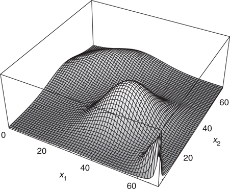
FIGURE 12.3
Combination of bearing and detection likelihood functions.

12.3 Multiple-Target Tracking without Contacts or Association (Unified Tracking)

In this section, the Bayesian tracking model for a single target is extended to multiple targets in a way that allows multiple-target tracking without calling contacts or performing data association.

12.3.1 Multiple-Target Motion Model

In Section 12.2, the prior knowledge about the single target’s state and its motion through the target state space S were represented in terms of a stochastic process {X(t); t ≥ 0} where X(t) is the target state at time t. This motion model is now generalized to multiple targets.

Begin the multiple-target tracking problem at time t = 0. The total number of targets is unknown but bounded by N¯¯¯ $\bar{N}$ , which is known. We assume a known bound on the number of targets because it allows us to simplify the presentation and produces no restriction in practice. Designate a region, R, which defines the boundary of the tracking problem. Activity outside of R has no importance. For example, we might be interested in targets having only a certain range of speeds or contained within a certain geographic region.

Add an additional state φ to the target state space S. If a target is not in the region R, it is considered to be in state φ. Let S⁺ = S ∪ {φ} be the extended state space for a single target and S⁺ = S⁺ × … × S⁺ be the joint target state space where the product is taken N¯¯¯ $\bar{N}$ times.

12.3.1.1 Multiple-Target Motion Process

Prior knowledge about the targets and their movements through the state space S⁺ is expressed as a stochastic process X = {X(t); t ≥ 0}. Specifically, let X(t) = (X₁(t), …, X_N(t)) be the state of the system at time t where X_n(t) ∊ S⁺ is the state of target n at time t. The term state of the system is used to mean the joint state of all the targets. The value of the random variable X_n(t) indicates whether target n is present in R and, if so, in what state. The number of components of X(t) with states not equal to φ at time t gives the number of targets present in R at time t. Assume that the stochastic process X is Markovian in the state space S⁺ and that the process has an associated transition function. Let q_k(s_k|s_k–1) = Pr{X(t_k) = s_k|X(t_k–1) = s_k–1} for k ≥ 1, and let q₀ be the probability (density) function for X(0). By the Markov assumption

P r {X (t 1) = s 1, \dots, X (t k) = s K} = \int Π k = 1 K q k (s k | s k - 1) q 0 (s 0) d s 0 (12.11)

$\begin{matrix} Pr {X (t_{1}) = s_{1}, \dots, X (t_{k}) = s_{K}} = \int Π_{k = 1}^{K} q_{k} (s_{k} | s_{k - 1}) q_{0} (s_{0}) d s_{0} & (12.11) \end{matrix}$

The state space S⁺ of the Markov process X has a measure associated with it. If the process S⁺ is a discrete space Markov chain, then the measure is discrete and integration becomes summation. If the space is continuous, then functions such as transition functions become densities on S⁺ with respect to that measure. If S⁺ has both continuous and discrete components, then the measure will be the product or mixture of discrete and continuous measures. The symbol ds will be used to indicate integration with respect to the measure on S⁺, whether it is discrete or not. When the measure is discrete, the integrals become summations. Similarly, the notation Pr indicates either probability or probability density as appropriate.

12.3.2 Multiple-Target Likelihood Functions

There is a set of sensors that report observations at a discrete sequence of possibly random times. These sensors may be of different types and may report different information. The sensors may report only when they have a contact or on a regular basis. Let Z(t, j) be an observation from sensor j at time t. Observations from sensor j take values in the measurement space H_j. Each sensor may have a different measurement space.

For each sensor j, assume that one can compute

P r {Z (t, j) = z | X (t) = s} for z \in H j and s \in S + (12.12)

$\begin{matrix} \begin{matrix} \begin{matrix} \begin{matrix} Pr {Z (t, j) = z | X (t) = s} & for \end{matrix} z \in H_{j} & and \end{matrix} & s \end{matrix} \in S^{+} & (12.12) \end{matrix}$

To compute the probabilities in Equation 12.12, one must know the distribution of the sensor response conditioned on the value of the state s. In contrast to Section 12.2, the likelihood functions in this section can depend on the joint state of all the targets. The relationship between the observation and the state s may be linear or nonlinear, and the probability distribution may be Gaussian or non-Gaussian.

Suppose that by time t, observations have been obtained at the set of discrete times 0 ≤ t₁ ≤ … ≤ t_K ≤ t. To allow for the possibility of receiving more than one sensor observation at a given time, let Y_k be the set of sensor observations received at time t_k. Let y_k denote a value of the random variable Y_k. Extend Equation 12.12 to assume that the following computation can be made

L k (y k | s) = P r {Y k = y k ∣ ∣ X (t k) = s} for s \in S + (12.13)

$\begin{matrix} L_{k} (y_{k} | s) = Pr {Y_{k} = y_{k} | X (t_{k}) = s} for s \in S^{+} & (12.13) \end{matrix}$

L_k(y_k|·) is called the likelihood function for the observation Y_k = y_k. The computation in Equation 12.13 can account for correlation among sensor responses if required.

Let Y(t) = (Y₁, Y₂, …, Y_K) and y = (y₁, …, y_K). Define L(y|s₁, …, s_K) = Pr{Y(t) = y|X(t₁) = s₁, …, X(t_K) = s_k}.

In parallel with Section 12.2, assume that

P r {Y (t) = y | X (u) = s (u), 0 \leq u \leq t} = L (y | s (t 1), \dots, s (t k)) (12.14)

$\begin{matrix} Pr {Y (t) = y | X (u) = s (u), 0 \leq u \leq t} = L (y | s (t_{1}), \dots, s (t_{k})) & (12.14) \end{matrix}$

and

L (y | s 1, \dots, s K) = Π k = 1 K L k (y k | s k) (12.15)

$\begin{matrix} L (y | s_{1}, \dots, s_{K}) = Π_{k = 1}^{K} L_{k} (y_{k} | s_{k}) & (12.15) \end{matrix}$

Equation 12.14 assumes that the distribution of the sensor response at the times {t_k, k = 1, …, K} depends only on the system states at those times. Equation 12.15 assumes independence of the sensor response distributions across the observation times. The effect of both assumptions is to assume that the sensor response at time t_k depends only on the system state at that time.

12.3.3 Posterior Distribution

For unified tracking, the tracking problem is equivalent to computing the posterior distribution on X(t) given Y(t). The posterior distribution of X(t) represents our knowledge of the number of targets present and their state at time t given Y(t). From this distribution point, estimates can be computed, when appropriate, such as maximum a posteriori probability estimates or means. Define q(s₁, …, s_K) = Pr{X(t₁) = s₁, …, X(t_K) = s_K} to be the prior probability (density) that the process X passes through the states s₁, …, s_K at times t₁, …, t_K. Let q₀ be the probability (density) function for X(0). By the Markov assumption

q (s 1, \dots, s K) = \int Π k = 1 K q k (s k | s k - 1) q 0 (s 0) d s 0 (12.16)

$\begin{matrix} q (s_{1}, \dots, s_{K}) = \int Π_{k = 1}^{K} q_{k} (s_{k} | s_{k - 1}) q_{0} (s_{0}) d s_{0} & (12.16) \end{matrix}$

Let p(t, s) = Pr{X(t) = s|Y(t)}. The function p(t, ·) gives the posterior distribution on X(t) given Y(t). By Bayes’ theorem,

p (t K, s K) = = P r { Y ( t K ) = y and X ( t k ) = s K } P r { Y ( t K ) = y } \int L ( y | s 1 , \dots , s K ) q ( s 1 , s 2 , \dots , s K ) d s 1 \dots d s K - 1 \int L ( y | s 1 , \dots , s K ) q ( s 1 , s 2 , \dots , s K ) d s 1 \dots d s K (12.17)

$\begin{matrix} p (t_{K}, s_{K}) = & \frac{\begin{matrix} \begin{matrix} Pr {Y (t_{K}) = y & and \end{matrix} & X (t_{k}) \end{matrix} = s_{K}}}{Pr {Y (t_{K}) = y}} \\ = & \frac{\int L (y | s_{1}, \dots, s_{K}) q (s_{1}, s_{2}, \dots, s_{K}) d s_{1} \dots {d s}_{K - 1}}{\int L (y | s_{1}, \dots, s_{K}) q (s_{1}, s_{2}, \dots, s_{K}) d s_{1} \dots {d s}_{K}} & (12.17) \end{matrix}$

12.3.4 Unified Tracking Recursion

Substituting Equations 12.15 and 12.16 into Equations 12.17 gives

p (t K, s K) = = 1 C ' \int Π k = 1 K L k (y k | s k) Π k = 1 K q k (s k | s k - 1) q 0 (s 0) d s 0 \dots d s K - 1 1 C ' L k (y k | s k) \int q K (s K | s K - 1) \times [\int Π k = 1 K - 1 L k (y k | s k) q k (s k | s k - 1) q 0 (s 0) d s 0 \dots d s K - 2] d s K - 1

$\begin{matrix} p (t_{K}, s_{K}) = & \frac{1}{C'} \int Π_{k = 1}^{K} L_{k} (y_{k} | s_{k}) Π_{k = 1}^{K} q_{k} (s_{k} | s_{k - 1}) q_{0} (s_{0}) d s_{0} \dots d s_{K - 1} \\ = & \frac{1}{C'} L_{k} (y_{k} | s_{k}) \int q_{K} (s_{K} | s_{K - 1}) \\ \times [\int Π_{k = 1}^{K - 1} L_{k} (y_{k} | s_{k}) q_{k} (s_{k} | s_{k - 1}) q_{0} (s_{0}) d s_{0} \dots d s_{K - 2}] d s_{K - 1} \end{matrix}$

and

p (t K' s K) = 1 C L K (y K | s K) \int q K (s K | s K - 1) p (t k - 1, s K - 1) d s K - 1 (12.18)

$\begin{matrix} p (t_{K'} s_{K}) = \frac{1}{C} L_{K} (y_{K} | s_{K}) \int q_{K} (s_{K} | s_{K - 1}) p (t_{k - 1}, s_{K - 1}) d s_{K - 1} & (12.18) \end{matrix}$

where C and C’ normalize p(t_K, ·) to be a probability distribution. Equation 12.18 provides a recursive method of computing p(t_K, ·). Specifically,

Unified tracking recursion

I n i t i a l i z e d i s t r i b u t i o n : p (t 0, s 0) = q 0 (s 0) for s 0 \in S + (12.19)

$\begin{matrix} \begin{matrix} Initialize distribution : p (t_{0}, s_{0}) = q_{0} (s_{0}) & for \end{matrix} s_{0} \in S^{+} & (12.19) \end{matrix}$

For k ≥ 1 and s_k ∊ S⁺,

P e r f o r m m o t i o n u p d a t e : p - (t k, s k) = \int q k (s k | s k - 1) p (t k - 1, s k - 1) d s k - 1 (12.20)

$\begin{matrix} Perform motion update : p^{-} (t_{k}, s_{k}) = \int q_{k} (s_{k} | s_{k - 1}) p (t_{k - 1}, s_{k - 1}) d s_{k - 1} & (12.20) \end{matrix}$

Compute likelihood function: L_k from the observation Y_k = y_k

P e r f o r m i n f o r m a t i o n u p d a t e : p (t k, s k) = 1 C L k (y k | s k) p - (t k, s k) (12.21)

$\begin{matrix} Perform information update : p (t_{k}, s_{k}) = \frac{1}{C} L_{k} (y_{k} | s_{k}) p^{-} (t_{k}, s_{k}) & (12.21) \end{matrix}$

12.3.4.1 Multiple-Target Tracking without Contacts or Association

The unified tracking recursion appears deceptively simple. The difficult part is performing the calculations in the joint state space of the N¯¯¯ $\bar{N}$ targets. Having done this, the combination of the likelihood functions defined on the joint state space with the joint distribution function of the targets automatically accounts for all possible association hypotheses without requiring explicit identification of these hypotheses. Section 12.4 demonstrates that this recursion produces the same joint posterior distribution as MHT does when the conditions for MHT are satisfied. However, the unified tracking recursion goes beyond MHT. One can use this recursion to perform multiple-target tracking when the notions of contact and association (notions required by MHT) are not meaningful. Examples of this are given in Section 5.3 of Ref. 3. Another example by Finn⁴ applies to tracking two aircraft targets with a monopulse radar when the aircrafts become so close together in bearing that their signals become unresolved. They merge inextricably at the radar receiver.

12.3.4.1.1 Merged Measurements

The problem tackled by Finn⁴ is an example of the difficulties caused by merged measurements. A typical example of merged measurements is when a sensor’s received signal is the sum of the signals from all the targets present. This can be the case with a passive acoustic sensor. Fortunately, in many cases the signals are separated in space or frequency so that they can be treated as separate signals. In some cases, two targets are so close in space (and radiated frequency) that it is impossible to distinguish which component of the received signal is due to which target. This is a case when the notion of associating a contact to a target is not well defined. Unified tracking will handle this problem correctly, but the computational load may be too onerous. In this case an MHT algorithm with special approximations could be used to provide an approximate but computationally feasible solution. See, for example, Ref. 5.

Section 12.4 presents the assumptions that allow contact association and multiple-target tracking to be performed by using MHT.

12.3.4.2 Summary of Assumptions for Unified Tracking Recursion

In summary, the assumptions required for the validity of the unified tracking recursion are

The number of targets is unknown but bounded by N¯¯¯ $\bar{N}$ .
S⁺ = S ∪ {ϕ} is the extended state space for a single target where ϕ indicates the target is not present. X_n(t) ∊ S⁺ is the state of the nth target at time t.
X(t) = (X₁(t), …, X_N(t)) is the state of the system at time t, and X = {X(t); t ≥ 0} is the stochastic process describing the evolution of the system over time. The process, X, is Markov in the state space S⁺ = S⁺ × … × S⁺ where the product is taken N¯¯¯ $\bar{N}$ times.
Observations occur at discrete (possibly random) times, 0 ≤ t₁ ≤ t₂ …. Let Y_k = y_k be the observation at time t_k, and let Y(t_K) = y_K = (y₁, …, y_K) be the first K observations. Then the following is true

P r {Y (t k) = = = y K | X (u) = s (u), 0 \leq u \leq t K} P r {Y (t K) = y K | X (t K) = s (t K), k = 1, \dots, K} Π k = 1 K L k (y k | s (t K))

$\begin{matrix} Pr {Y (t_{k}) = & y_{K} | X (u) = s (u), 0 \leq u \leq t_{K}} \\ = & Pr {Y (t_{K}) = y_{K} | X (t_{K}) = s (t_{K}), k = 1, \dots, K} \\ = & Π_{k = 1}^{K} L_{k} (y_{k} | s (t_{K})) \end{matrix}$

12.4 Multiple-Hypothesis Tracking

In classical multiple-target tracking, the problem is divided into two steps: (1) association and (2) estimation. Step 1 associates contacts with targets. Step 2 uses the contacts associated with each target to produce an estimate of that target’s state. Complications arise when there is more than one reasonable way to associate contacts with targets. The classical approach to this problem is to form association hypotheses and to use MHT, which is the subject of this section. In this approach, alternative hypotheses are formed to explain the source of the observations. Each hypothesis assigns observations to targets or false alarms. For each hypothesis, MHT computes the probability that it is correct. This is also the probability that the target state estimates that result from this hypothesis are correct. Most MHT algorithms display only the estimates of target state associated with the highest probability hypothesis.

The model used for the MHT problem is a generalization of the one given by Reid⁶ and Mori et al.⁷ Section 12.4.3.3 presents the recursion for general MHT. This recursion applies to problems that are nonlinear and non-Gaussian as well as to standard linear-Gaussian situations. In this general case, the distributions on target state may fail to be independent of one another (even when conditioned on an association hypothesis) and may require a joint state space representation. This recursion includes a conceptually simple Bayesian method of computing association probabilities. Section 12.4.4 discusses the case where the target distributions (conditioned on an association hypothesis) are independent of one another. Section 12.4.4.2 presents the independent MHT recursion that holds when these independence conditions are satisfied. Note that not all tracking situations satisfy these independence conditions.

Numerous books and articles on multiple-target tracking examine in detail the many variations and approaches to this problem. Many of these discuss the practical aspects of implementing multiple-target trackers and compare approaches. See, for example, Refs 1 and 6–13. With the exception of Ref. 7 these references focus primarily on the linear-Gaussian case.

In addition to the full or classical MHT as defined by Reid⁶ and Mori et al.,⁷ a number of approximations are in common use for finding solutions to tracking problems. Examples include joint probabilistic data association⁹ and probabilistic MHT.¹⁴ Rather than solve the full MHT, Poore¹⁵ attempts to find the data association hypothesis (or the n hypotheses) with the highest likelihood. The tracks formed from this hypothesis then become the solution. Poore does this by providing a window of scans in which contacts are free to float among hypotheses. The window has a constant width and always includes the latest scan. Eventually contacts from older scans fall outside the window and become assigned to a single hypothesis. This type of hypothesis management is often combined with a nonlinear extension of Kalman filtering called an interactive multiple model Kalman filter.¹⁶

Section 12.4.1 presents a description of general MHT. Note that general MHT requires many more definitions and assumptions than unified tracking.

12.4.1 Contacts, Scans, and Association Hypotheses

This discussion of MHT assumes that sensor responses are limited to contacts.

12.4.1.1 Contacts

A contact is an observation that consists of a called detection and a measurement. In practice, a detection is called when the signal-to-noise ratio at the sensor crosses a predefined threshold. The measurement associated with a detection is often an estimated position for the object generating the contact. Limiting the sensor responses to contacts restricts responses to those in which the signal level of the target, as seen at the sensor, is high enough to call a contact. Section 12.6 demonstrates how tracking can be performed without this assumption being satisfied.

12.4.1.2 Scans

This discussion further limits the class of allowable observations to scans. The observation Y_k at time t_k is a scan if it consists of a set C_k of contacts such that each contact is associated with at most one target, and each target generates at most one contact (i.e., there are no merged or split measurements). Some of these contacts may be false alarms, and some targets in R might not be detected on a given scan.

More than one sensor group can report a scan at the same time. In this case, the contact reports from each sensor group are treated as separate scans with the same reporting time. As a result, t_k+1 = t_k. A scan can also consist of a single contact report.

12.4.1.3 Data Association Hypotheses

To define a data association hypothesis, h, let

C_j = set of contacts of the jth scan

H(k) = set of all contacts reported in the first k scans

Note that

H (k) = \cup j = 1 k C j

$H (k) = \cup_{j = 1}^{k} C_{j}$

A data association hypothesis, h, on K(k) is a mapping

h : K (k) \to {0, 1, \dots, N ¯ ¯ ¯}

$h : K (k) \to {0, 1, \dots, \bar{N}}$

such that h(c) = n > 0 means contact c is associated to target n, h(c) = 0 means contact c is associated to a false alarm, and no two contacts from the same scan are associated to the same target.

Let H(k) = set of all data association hypotheses on H(k). A hypothesis h on K(k) partitions K(k) into sets U(n) for n=0,1,…,N¯¯¯ $n = 0, 1, \dots, \bar{N}$ where U(n) is the set of contacts associated to target n for n > 0 and U(0) is the set of contacts associated to false alarms.

12.4.1.4 Scan Association Hypotheses

Decomposing a data association hypothesis h into scan association hypotheses is convenient. For each scan Y_k, let M_k = the number of contacts in scan k, Γ_k = the set of all functions γ:{1,…,Mk}→{0,…,N¯¯¯} $γ : {1, \dots, M_{k}} \to {0, \dots, \bar{N}}$ such that no two contacts are assigned to the same positive number. If γ(m) = 0, then contact m is associated to a false alarm. If γ(m) = n > 0, then contact m is associated to target n.

A function γΓ_k is called a scan association hypothesis for the kth scan, and Γ_k is the set of scan association hypotheses for the kth scan. For each contact, a scan association hypothesis specifies which target generated the contact or that the contact was due to a false alarm.

Consider a data association hypothesis h_K ∊ H(K). Think of h_K as being composed of K scan association hypotheses {γ₁, …, γ_K} where γ_k is the association hypothesis for the kth scan of contacts. The hypothesis h_K ∊ H(K) is the extension of the hypothesis h_K–1 = {γ₁, …, γ_k–1} ∊ H(K – 1). That is, h_K is composed of h_K–1 plus γ_K. This can be written as h_K = h_k−1 ∧ γ_K.

12.4.2 Scan and Data Association Likelihood Functions

The correctness of the scan association hypothesis γ is equivalent to the occurrence of the event “the targets to which γ associates contacts generate those contacts.” Calculating association probabilities requires the ability to calculate the probability of a scan association hypothesis being correct. In particular, we must be able to calculate the probability of the event {γ ∧ Y_K = y_K}, where {γ ∧ Y_K = y_K} denotes the conjunction or intersection of the events γ and Y_k = y_k.

12.4.2.1 Scan Association Likelihood Function

Assume that for each scan association hypothesis γ, one can calculate the scan association likelihood function

l k (γ \land Y k = y k | s k) = = P r {γ \land Y k = y k | X (t k) = s k} P r {Y k = y k | γ \land X (t k) = s k} P r {γ | X (t k) = s k} for s k \in S + (12.22)

$\begin{matrix} l_{k} (γ \land Y_{k} = y_{k} | s_{k}) = & Pr {γ \land Y_{k} = y_{k} | X (t_{k}) = s_{k}} \\ = & \begin{matrix} \begin{matrix} Pr {Y_{k} = y_{k} | γ \land X (t_{k}) = s_{k}} Pr {γ | X (t_{k}) = s_{k}} \end{matrix} & for s_{k} \end{matrix} \in S^{+} & (12.22) \end{matrix}$

The factor Pr{γ|X(t_k) = s_k} is the prior probability that the scan association γ is the correct one. We normally assume that this probability does not depend on the system state s_k, so that one may write

l k (γ \land Y k = y k | s k) = P r {Y k = y k | γ \land X (t k) = s k} P r {γ} for s k \in S + (12.23)

$\begin{matrix} \begin{matrix} l_{k} (γ \land Y_{k} = y_{k} | s_{k}) = Pr {Y_{k} = y_{k} | γ \land X (t_{k}) = s_{k}} Pr {γ} & for \end{matrix} s_{k} \in S^{+} & (12.23) \end{matrix}$

Note that l_k(γ ∧ Y_K = y_k|⋅) is not, strictly speaking, a likelihood function because γ is not an observation. Nevertheless, it is called a likelihood function because it behaves like one. The likelihood function for the observation Y_k = y_k is

l k (y k | s k) = P r {Y k = y k | X (t k) = s k} = \sum γ \in Γ k l k (γ \land Y k = y k | s k) for s k \in S + (12.24)

$\begin{matrix} \begin{matrix} l_{k} (y_{k} | s_{k}) = Pr {Y_{k} = y_{k} | X (t_{k}) = s_{k}} = \sum_{γ \in Γ_{k}} l_{k} (γ \land Y_{k} = y_{k} | s_{k}) & for \end{matrix} s_{k} \in S^{+} & (12.24) \end{matrix}$

12.4.2.1.1 Scan Association Likelihood Function Example

Consider a tracking problem where detections, measurements, and false alarms are generated according to the following model. The target state, s, is composed of an l-dimensional position component, z, and an l-dimensional velocity component, v, in a Cartesian coordinate space, so that s = (z, v). The region of interest, R, is finite and has volume V in the l-dimensional position component of the target state space. There are at most N¯¯¯ $\bar{N}$ targets in R.

Detections and measurements. If a target is located at z, then the probability of its being detected on a scan is P_d(z). If a target is detected then a measurement Y is obtained where Y = z + ε and ε ~ N(0, Σ). Let η(y, z, Σ) be the density function for a N(z, Σ) random variable evaluated at y. Detections and measurements occur independently for all targets.

False alarms. For each scan, false alarms occur as a Poisson process in the position space with density ρ. Let Φ be the number of false alarms in a scan, then

Pr {Φ = j} = ( ρ V ) j j ! for j = 0, 1, \dots

$\begin{matrix} Pr {Φ = j} = \frac{(ρ V)^{j}}{j!} & for j \end{matrix} = 0, 1, \dots$

Scan. Suppose that a scan of M measurements is received y = (y₁, …, y_M) and γ is a scan association. Then γ specifies which contacts are false and which are true. In particular, if γ(m) = n > 0, measurement m is associated to target n. If γ(m) = 0, measurement m is associated to a false target. No target is associated with more than one contact. Let

φ(γ) = the number of contacts associated to false alarms

I(γ) = {n : γ associates no contact in the scan to target n} = the set of targets that have no contacts associated to them by γ

Scan Association Likelihood Function. Assume that the prior probability is the same for all scan associations, so that for some constant G, Pr{γ} = G for all γ. The scan association likelihood function is

l (γ \land y | s = (z, v)) = G ( ρ V ) ϕ ( γ ) ϕ ( γ ) ! V ϕ ( γ ) e - ρ V Π {m : γ (m) > 0} P D (z γ (m)) η (y m, z γ (m)' Σ) Π n \in I (γ) (1 - P D (z n)) (12.25)

$\begin{matrix} l (γ \land y| s = (z, v)) = \frac{G {(ρ V)}^{ϕ (γ)}}{ϕ (γ)! V^{ϕ (γ)}} e^{- ρ V} \underset{{m : γ (m) > 0}}{Π} P_{D} (z_{γ (m)}) η (y_{m}, z_{γ (m)'} Σ) \underset{n \in I (γ)}{Π} (1 - P_{D} (z_{n})) & (12.25) \end{matrix}$

12.4.2.2 Data Association Likelihood Function

Recall that Y(t_K) = y_K is the set of observations (contacts) contained in the first K scans and H(K) is the set of data association hypotheses defined on these scans. For h ∊ H(K), Pr{h ∧ Y(t_k) = y_K|X(u) = s_u, 0 ≤ u ≤ t_k} is the likelihood of {h ∧ Y(t_k) = y_K}, given {X(u) = s_u, 0 ≤ u ≤ t_K}. Technically, this is not a likelihood function either, but it is convenient and suggestive to use this terminology. As with the observation likelihood functions, assume that

P r {h \land Y (t K) = = y K | X (u) = s (u), 0 \leq u \leq t k} P r {h \land Y (t K) = y K | X (t k) = s (t k), k = 1, \dots, K} (12.26)

$\begin{matrix} \begin{matrix} Pr {h \land Y (t_{K}) = & y_{K} | X (u) = s (u), 0 \leq u \leq t_{k}} \\ = & Pr {h \land Y (t_{K}) = y_{K} | X (t_{k}) = s (t_{k}), k = 1, \dots, K} \end{matrix} & (12.26) \end{matrix}$

In addition, assuming that the scan association likelihoods are independent, the data association likelihood function becomes

P r {h \land Y (t k) = y K | X (t k) = s k, k = 1, \dots, K} = Π k = 1 K l k (γ k \land Y k = y k | s k) (12.27)

$\begin{matrix} Pr {h \land Y (t_{k}) = y_{K} | X (t_{k}) = s_{k}, k = 1, \dots, K} = Π_{k = 1}^{K} l_{k} (γ_{k} \land Y_{k} = y_{k} | s_{k}) & (12.27) \end{matrix}$

where y_K = (y₁, …, y_K) and h = {γ₁, …, γ_k}.

12.4.3 General Multiple-Hypothesis Tracking

Conceptually, MHT proceeds as follows. It calculates the posterior distribution on the system state at time t_K, given that data association hypothesis h is true, and the probability, α(h), that hypothesis h is true for each h ∊ H(K). That is, it computes

p (t K, s K | h) \equiv P r {X (t K) = s K | h \land Y (t K) = y K} (12.28)

$\begin{matrix} p (t_{K}, s_{K} | h) \equiv Pr {X (t_{K}) = s_{K} | h \land Y (t_{K}) = y_{K}} & (12.28) \end{matrix}$

and

α (h) \equiv P r {h | Y (t K) = y K} = P r { h \land Y ( t K ) = y K } P r { Y ( t K ) = y K } for each h \in H (K) (12.29)

$\begin{matrix} \begin{matrix} α (h) \equiv Pr {h | Y (t_{K}) = y_{K}} = \frac{Pr {h \land Y (t_{K}) = y_{K}}}{Pr {Y (t_{K}) = y_{K}}} & for each h \end{matrix} \in H (K) & (12.29) \end{matrix}$

Next, MHT can compute the Bayesian posterior on system state by

p (t k, s K) = Σ h \in H (K) α (h) p (t K, s K | h) (12.30)

$\begin{matrix} p (t_{k}, s_{K}) = \underset{h \in H (K)}{Σ} α (h) p (t_{K}, s_{K} | h) & (12.30) \end{matrix}$

Subsequent sections show how to compute p(t_K, s_K|h) and α(h) in a joint recursion.

A number of difficulties are associated with calculating the posterior distribution in Equation 12.30. First, the number of data association hypotheses grows exponentially as the number of contacts increases. Second, the representation in Equation 12.30 is on the joint N¯¯¯ $\bar{N}$ -fold target state space, a state space that is dauntingly large for most values of N¯¯¯ $\bar{N}$ . Even when the size of the joint state space is not a problem, displaying and understanding the joint distribution is difficult.

Most MHT algorithms overcome these problems by limiting the number of hypotheses carried, displaying the distribution for only a small number of the highest probability hypotheses—perhaps only the highest. Finally, for a given hypothesis, they display the marginal distribution on each target, rather than the joint distribution. (Note, specifying a data association hypothesis specifies the number of targets present in R.) Most MHT implementations make the linear-Gaussian assumptions that produce Gaussian distributions for the posterior on a target state. The marginal distribution on a two-dimensional target position can then be represented by an ellipse. It is usually these ellipses, one for each target, that are displayed by an MHT to represent the tracks corresponding to a hypothesis.

12.4.3.1 Conditional Target Distributions

Distributions conditioned on the truth of a hypothesis are called conditional target distributions. The distribution p(t_K, ·|h) in Equation 12.28 is an example of a conditional joint target state distribution. These distributions are always conditioned on the data received (e.g., Y(t_K) = y_K), but this conditioning does not appear in our notation, p(t_K, s_K|h).

Let h_K = {γ₁, …, γ_K}, then

p (t K, s K | h K) = = P r {X (t K) = s K | h K \land Y (t K) = y K} P r { ( X ( t K ) = s K ) \land h K \land ( Y ( t K ) = y K ) } P r { h K \land Y ( t K ) = y K }

$\begin{matrix} p (t_{K}, s_{K} | h_{K}) = & Pr {X (t_{K}) = s_{K} | h_{K} \land Y (t_{K}) = y_{K}} \\ = & \frac{Pr {(X (t_{K}) = s_{K}) \land h_{K} \land (Y (t_{K}) = y_{K})}}{Pr {h_{K} \land Y (t_{K}) = y_{K}}} \end{matrix}$

and by Equation 12.11 and the data association likelihood function in Equation 12.27,

P r {(X (t K) = = s K) \land h K \land (Y (t k) = y K)} \int {Π k = 1 K l k (γ k \land Y k = y K | s k) Π k = 1 K q k (s k | s k - 1) q 0 (s 0)} d s 0 d s 1 \dots d s k - 1 (12.31)

$\begin{matrix} Pr {(X (t_{K}) = & s_{K}) \land h_{K} \land (Y (t_{k}) = y_{K})} \\ = & \int {Π_{k = 1}^{K} l_{k} (γ_{k} \land Y_{k} = y_{K} | s_{k}) Π_{k = 1}^{K} q_{k} (s_{k} | s_{k - 1}) q_{0} (s_{0})} d s_{0} {d s}_{1} \dots d s_{k - 1} & (12.31) \end{matrix}$

Thus,

p (t K, s K | h K) = 1 C ( h K ) \int {Π k = 1 K l k (γ k \land Y k = y k | s k) q k (s k | s k - 1)} q 0 (s 0) d s 0 d s 1 \dots d s k - 1 (12.32)

$\begin{matrix} p (t_{K}, s_{K} | h_{K}) = \frac{1}{C (h_{K})} \int {Π_{k = 1}^{K} l_{k} (γ_{k} \land Y_{k} = y_{k} | s_{k}) q_{k} (s_{k} | s_{k - 1})} q_{0} (s_{0}) d s_{0} d s_{1} \dots d s_{k - 1} & (12.32) \end{matrix}$

where C(h_K) is the normalizing factor that makes p(t_K, ·|h_K) a probability distribution. Of course

C (h K) = = \int {Π k = 1 K l k (γ k \land Y k = y k | s k) q k (s k | s k - 1)} q 0 (s 0) d s 0 d s 1 \dots d s k P r {h K \land Y (t K) = y K} (12.33)

$\begin{matrix} C (h_{K}) = & \int {Π_{k = 1}^{K} l_{k} (γ_{k} \land Y_{k} = y_{k} | s_{k}) q_{k} (s_{k} | s_{k - 1})} q_{0} (s_{0}) d s_{0} d s_{1} \dots d s_{k} \\ = & Pr {h_{K} \land Y (t_{K}) = y_{K}} & (12.33) \end{matrix}$

12.4.3.2 Association Probabilities

Sections 4.2.1 and 4.2.2 of Ref. 3 show that

α (h) = P r {h | Y (t K) = y K} = P r { h \land Y ( t K ) = y K } P r { Y ( t K ) = y K } = C ( h ) Σ h ' \in H ( K ) C ( h ' ) for h \in H (K) (12.34)

$\begin{matrix} \begin{matrix} α (h) = Pr {h | Y (t_{K}) = y_{K}} = \frac{Pr {h \land Y (t_{K}) = y_{K}}}{Pr {Y (t_{K}) = y_{K}}} = \frac{C (h)}{\underset{h' \in H (K)}{Σ} C (h')} & for h \in H (K) \end{matrix} & (12.34) \end{matrix}$

12.4.3.3 General MHT Recursion

Section 4.2.3 of Ref. 3 provides the following general MHT recursion for calculating conditional target distributions and hypothesis probabilities.

General MHT recursion

Intialize: Let H(0) = {h₀}, where h₀ is the hypothesis with no associations. Set

$α (h 0) = 1 and p (t 0, s 0 | h 0) = q 0 (s 0) for s 0 \in S +$ $\begin{matrix} \begin{matrix} \begin{matrix} α (h_{0}) = 1 & and \end{matrix} & p (t_{0}, s_{0} | h_{0}) \end{matrix} = q_{0} (s_{0}) & for \end{matrix} s_{0} \in S^{+}$
Compute conditional target distributions: For k = 1, 2, …, compute

$p - (t k, s k | h k - 1) = \int q k (s k | s k - 1) p (t k - 1, s k - 1 | h k - 1) d s k - 1 for h k - 1 \in H (k - 1) (12.35)$ $\begin{matrix} \begin{matrix} p^{-} (t_{k}, s_{k} | h_{k - 1}) = \int q_{k} (s_{k} | s_{k - 1}) p (t_{k - 1}, s_{k - 1} | h_{k - 1}) d s_{k - 1} & for \end{matrix} h_{k - 1} \in H (k - 1) & (\begin{matrix} 12.35 \end{matrix}) \end{matrix}$

For h_k = h_k−1 ∧ γ_k ∊ H(k), compute

$β (h k) = α (h k - 1) \int l k (γ k \land Y k = y k | s k) p - (t k, s k | h k - 1) d s k (12.36)$ $\begin{matrix} β (h_{k}) = α (h_{k - 1}) \int l_{k} (γ_{k} \land Y_{k} = y_{k} | s_{k}) p^{-} (t_{k}, s_{k} | h_{k - 1}) d s_{k} & (12.36) \end{matrix}$

$p (t k, s k | h k) = α ( h k - 1 ) β ( h k ) l k (γ k \land Y k = y k | s k) p - (t k, s k | h k - 1) for s k \in S + (12.37)$ $\begin{matrix} \begin{matrix} p (t_{k}, s_{k} | h_{k}) = \frac{α (h_{k - 1})}{β (h_{k})} l_{k} (γ_{k} \land Y_{k} = y_{k} | s_{k}) p^{-} (t_{k}, s_{k} | h_{k - 1}) & for s_{k} \end{matrix} \in S^{+} & (12.37) \end{matrix}$
Compute association probabilities: For k = 1, 2, …, compute

$α (h k) = β ( h k ) Σ h \in H ( k ) β ( h ) for h K \in H (K) (12.38)$ $\begin{matrix} \begin{matrix} α (h_{k}) = \frac{β (h_{k})}{\underset{h \in H (k)}{Σ} β (h)} & for h_{K} \in H (K) \end{matrix} & (12.38) \end{matrix}$

12.4.3.4 Summary of Assumptions for General MHT Recursion

In summary, the assumptions required for the validity of the general MHT recursion are

The number of targets is unknown but bounded by N¯¯¯ $\bar{N}$ .
S⁺ = S ∪ {ϕ} is the extended state space for a single target, where ϕ indicates that the target is not present.
X_n(t) ∊ S⁺ is the state of the nth target at time t.
X(t)=(X)1(t),…,XN¯¯¯(t)) $X (t) = (X)_{1} (t), \dots, X_{\bar{N}} (t))$ is the state of the system at time t, and X = {X(t); t ≥ 0} is the stochastic process describing the evolution of the system over time. The process, X, is Markov in the state space S⁺ = S⁺ × … × S⁺ where the product is taken N¯¯¯ $\bar{N}$ times.
Observations occur as contacts in scans. Scans are received at discrete (possibly random) times 0 ≤ t₁ ≤ t₂…. Let Y_k = y_k be the scan (observation) at time t_k, and let Y(t_k) = y_K ≡ (y₁, …, y_k) be the set of contacts contained in the first K scans. Then, for each data association hypothesis h ∊ H(K), the following is true:

$P r {h \land Y (t k) = = y K | X (u) = s (u), 0 \leq u \leq t K} P r {h \land Y (t K) = y K | X (t K) = s (t K), k = 1, \dots, K}$ $\begin{matrix} Pr {h \land Y (t_{k}) = & y_{K} | X (u) = s (u), 0 \leq u \leq t_{K}} \\ = & Pr {h \land Y (t_{K}) = y_{K} | X (t_{K}) = s (t_{K}), k = 1, \dots, K} \end{matrix}$
For each scan association hypothesis γ at time t_k, there is a scan association likelihood function

$l k (γ \land Y k = y k | s k) = P r {γ \land Y k = y k | X (t k) = s k}$ $l_{k} (γ \land Y_{k} = y_{k} | s_{k}) = Pr {γ \land Y_{k} = y_{k} | X (t_{k}) = s_{k}}$
Each data association hypothesis, h ∊ H(K), is composed of scan association hypotheses so that h = {γ₁, …, γ_K} where γ_k is a scan association hypothesis for scan k.
The likelihood function for the data association hypothesis h = {γ₁, …, γ_K} satisfies

$P r {h \land Y (t K) = y K | X (u) = s (u), 0 \leq u \leq t K} = Π k = 1 K l k (γ k \land Y k = y k | s (t K))$ $Pr {h \land Y (t_{K}) = y_{K} | X (u) = s (u), 0 \leq u \leq t_{K}} = Π_{k = 1}^{K} l_{k} (γ_{k} \land Y_{k} = y_{k} | s (t_{K}))$

12.4.4 Independent Multiple-Hypothesis Tracking

The decomposition of the system state distribution into a sum of conditional target distributions is most useful when the conditional distributions are the product of independent single-target distributions. This section presents a set of conditions under which this happens and restates the basic MHT recursion for this case.

12.4.4.1 Conditionally Independent Scan Association Likelihood Functions

Prior to this section no special assumptions were made about the scan association likelihood function l_k(γ ∧ Y_k = y_k|s_k) = Pr{γ ∧ Y_k = y_k|X(t_k) = s_k} for s_k ∊ S⁺. In many cases, however, the joint likelihood of a scan observation and a data association hypothesis satisfies an independence assumption when conditioned on a system state.

The likelihood of a scan observation Y_k = y_k obtained at time t_k is conditionally independent, if and only if, for all scan association hypotheses γ ∊ Γ_k,

l k (γ \land Y k = y k | s k) = = P r {γ \land Y k = y k | X (t k) = s k} g γ 0 (y k) Π n = 1 N ¯ ¯ ¯ g γ n (y k, x n) for s k = (x 1, \dots, x N ¯ ¯ ¯) (12.39)

$\begin{matrix} l_{k} (γ \land Y_{k} = y_{k} | s_{k}) = & Pr {γ \land Y_{k} = y_{k} | X (t_{k}) = s_{k}} \\ = & \begin{matrix} \begin{matrix} g_{0}^{γ} (y_{k}) Π_{n = 1}^{\bar{N}} g_{n}^{γ} (y_{k}, x_{n}) \end{matrix} & for s_{k} = (x_{1}, \dots, x_{\bar{N}}) \end{matrix} & (12.39) \end{matrix}$

for some functions gγn,n=0,…,N¯¯¯ $g_{n}^{γ}, n = 0, \dots, \bar{N}$ , where gγ0 $g_{0}^{γ}$ can depend on the scan data but not s_k.

Equation 12.39 shows that conditional independence means that the probability of the joint event {γ ∧ Y_k = y_k}, conditioned on X(tk)=(x1,…,xN¯¯¯) $X (t_{k}) = (x_{1}, \dots, x_{\bar{N}})$ , factors into a product of functions that each depend on the state of only one target. This type of factorization occurs when the component of the response due to each target is independent of all other targets. As an example, the scan association likelihood in Equation 12.25 is conditionally independent. This can be verified by setting

g γ 0 (y) = G ( ρ V ) ϕ ( γ ) ϕ ( γ ) ! V ϕ ( γ ) = G ρ ϕ ( γ ) ϕ ( γ ) !

$g_{0}^{γ} (y) = \frac{G {(ρ V)}^{ϕ (γ)}}{ϕ (γ)! V^{ϕ (γ)}} = \frac{{G ρ}^{ϕ (γ)}}{ϕ (γ)!}$

and for n=1,…,N¯¯¯ $n = 1, \dots, \bar{N}$

g γ n (y, z n) = {P d (z n) η (y m, z n, n) 1 - P d (z n) if γ (m) = n for some m if γ (m) \neq n for all m

$g_{n}^{γ} (y, z_{n}) = {\begin{matrix} P_{d} (z_{n}) η (y_{m}, z_{n}, n) & if γ (m) = n for some m \\ 1 - P_{d} (z_{n}) & if γ (m) \neq n for all m \end{matrix}$

Conditional independence implies that the likelihood function for the observation Y_k = y_k is given by

L k (Y k = y k | X (t k) = = (x 1, \dots, x N ¯ ¯ ¯)) Σ γ \in Γ k g γ 0 (y k) Π n = 1 N ¯ ¯ ¯ g γ n (y k, x n) for all (x 1, \dots, x N ¯ ¯ ¯) \in S + (12.40)

$\begin{matrix} L_{k} (Y_{k} = y_{k} | X (t_{k}) = & (x_{1}, \dots, x_{\bar{N}})) \\ = & \begin{matrix} \begin{matrix} \underset{γ \in Γ_{k}}{Σ} g_{0}^{γ} (y_{k}) Π_{n = 1}^{\bar{N}} g_{n}^{γ} (y_{k}, x_{n}) \end{matrix} & for all (x_{1}, \dots, x_{\bar{N}}) \in S^{+} \end{matrix} & (12.40) \end{matrix}$

The assumption of conditional independence of the observation likelihood function is implicit in most multiple-target trackers. The notion of conditional independence of a likelihood function makes sense only when the notions of contact and association are meaningful. As noted in Section 12.3, there are cases in which these notions do not apply. For these cases, the scan association likelihood function will not satisfy Equation 12.39.

Under the assumption of conditional independence, the Independence Theorem, discussed in Section 12.4.4.1.1, says that conditioning on a data association hypothesis allows the multiple-target tracking problem to be decomposed into N¯¯¯ $\bar{N}$ independent single-target problems. In this case, conditioning on a hypothesis greatly simplifies the joint tracking problem. In particular, no joint state space representation of the target distributions is required when they are conditional on a data association hypothesis.

12.4.4.1.1 Independence Theorem

Suppose that (1) the assumptions of Section 12.4.3.4 hold, (2) the likelihood functions for all scan observations are conditionally independent, and (3) the prior target motion processes, {X_n(t); t ≥ 0} for n = 1, …, N¯¯¯ $\bar{N}$ are mutually independent. Then the posterior system state distribution conditioned on the truth of a data association hypothesis is the product of independent distributions on the targets.

Proof. The proof of this theorem is given in Section 4.3.1 of Ref. 3.

Let Y(t) = {Y₁, Y₂, …, y_K(t)} be scan observations that are received at times 0 ≤ t₁ ≤, …, ≤ t_k ≤ t, where K = K(t), and let H(k) be the set of all data association hypotheses on the first k scans. Define p_n(t_k, x_n|h) = Pr{X_n(t_k) = x_n|h} for x_n ∊ S⁺, k = 1, …, K, and n=1,…,N¯¯¯ $n = 1, \dots, \bar{N}$ . Then by the independence theorem,

p (t k, s k | h) = Π n p n (t k, x n | h) for h \in H (k) and s k = (x 1, \dots, x N ¯ ¯ ¯) \in S + (12.41)

$\begin{matrix} \begin{matrix} \begin{matrix} \begin{matrix} p (t_{k}, s_{k} | h) = \underset{n}{Π} p_{n} (t_{k}, x_{n} | h) & for h \end{matrix} \in H (k) & and \end{matrix} & s_{k} \end{matrix} = (x_{1}, \dots, x_{\bar{N}}) \in S^{+} & (12.41) \end{matrix}$

Joint and Marginal Posteriors. From Equation 12.30 the full Bayesian posterior on the joint state space can be computed as follows:

p (t K, s K) = = Σ h \in H (K) α (h) p (t K, s k | h) Σ h \in H (K) α (h) Π n p n (t K, x n | h) for s K = (x 1, \dots, x N ¯ ¯ ¯) \in S + (12.42)

$\begin{matrix} p (t_{K}, s_{K}) = & \underset{h \in H (K)}{Σ} α (h) p (t_{K}, s_{k} | h) \\ = & \begin{matrix} \begin{matrix} \underset{h \in H (K)}{Σ} α (h) \underset{n}{Π} p_{n} (t_{K}, x_{n} | h) \end{matrix} & for s_{K} = (x_{1}, \dots, x_{\bar{N}}) \in S^{+} \end{matrix} & (12.42) \end{matrix}$

Marginal posteriors can be computed in a similar fashion. Let p¯n(tk,⋅) ${\bar{p}}_{n} (t_{k}, \cdot)$ be the marginal posterior on X_n(t_K) for n=1,…,N¯¯¯ $n = 1, \dots, \bar{N}$ . Then

p ¯ n (t K, x n) = = = \int [Σ h \in H (K) α (h) Π l = 1 N ¯ ¯ ¯ p 1 (t K, x 1 | h)] Π l \neq n d x l Σ h \in H (K) α (h) p n (t K, x n | h) \int Π l \neq n p 1 (t K, x l | h) d x l Σ h \in H (K) α (h) p n (t K, x n | h) for n = 1, \dots, N ¯ ¯ ¯

$\begin{matrix} {\bar{p}}_{n} (t_{K}, x_{n}) = & \int [\underset{h \in H (K)}{Σ} α (h) Π_{l = 1}^{\bar{N}} p_{1} (t_{K}, x_{1} | h)] \underset{l \neq n}{Π} {dx}_{l} \\ = & \underset{h \in H (K)}{Σ} α (h) p_{n} (t_{K}, x_{n} | h) \int \underset{l \neq n}{Π} p_{1} (t_{K}, x_{l} | h) {dx}_{l} \\ = & \begin{matrix} \begin{matrix} \underset{h \in H (K)}{Σ} α (h) p_{n} (t_{K}, x_{n} | h) \end{matrix} & for \end{matrix} n = 1, \dots, \bar{N} \end{matrix}$

Thus, the posterior marginal distribution on target n may be computed as the weighted sum over n of the posterior distribution for target n conditioned on h.

12.4.4.2 Independent MHT Recursion

Let q₀(n, x) = Pr{X_n(0) = x} and q_k(x|n, x’) = Pr{X_n(t_k) = x|X_n(t_k–1) = x’}. Under the assumptions of the independence theorem, the motion models for the targets are independent, and qn(sk|sk−1)=Πnqk(xn|n,x′n) $q_{n} (s_{k} | s_{k - 1}) = \underset{n}{Π} q_{k} (x_{n} | n, x_{n}^{'})$ where sk=(x1,…,xN¯¯¯) $s_{k} = (x_{1}, \dots, x_{\bar{N}})$ and sk−1=(x′1,…,x′N¯¯¯) $s_{k - 1} = (x_{1}^{'}, \dots, x_{\bar{N}}^{'})$ . As a result, the transition density, q_k(s_k|s_k–1), factors just as the likelihood function does. This produces the independent MHT recursion.

Independent MHT recursion

Intialize: Let H(0) = {h₀} where h₀ is the hypothesis with no associations. Set

$α (h 0) = 1 and p n (t 0, s 0 | h 0) = q 0 (n, s 0) for s 0 \in S + and n = 1, \dots, N ¯ ¯ ¯$ $\begin{matrix} \begin{matrix} \begin{matrix} \begin{matrix} \begin{matrix} α (h_{0}) = 1 & and \end{matrix} & p_{n} \end{matrix} (t_{0}, s_{0} | h_{0}) = q_{0} (n, s_{0}) & for \end{matrix} s_{0} \in S^{+} & and \end{matrix} & n = 1, \dots, \bar{N} \end{matrix}$
Compute conditional target distributions: For k = 1, 2, …, do the following: For each h_k ∊ H(k), find h_k–1 ∊ H(k – 1) and γ ∊ Γ_k, such that h_k = h_k−1 ∧ γ. Then compute

$p - n (t k, x | h k - 1) = \int S + q k (x | n, x') p n (t k - 1, x' | h k - 1) d x' for = 1, \dots, N ¯ ¯ ¯ and n = 1, \dots, N ¯ ¯ ¯ p (t k, s k | h k) = Π n p n (t k, x n | h k) for s k = (x 1, \dots, x N ¯ ¯ ¯) \in S + (12.43)$ $\begin{matrix} \begin{matrix} \begin{matrix} p_{n}^{-} (t_{k}, x | h_{k - 1}) = \int_{S^{+}} q_{k} (x | n, x^{'}) p_{n} (t_{k - 1}, x^{'} | h_{k - 1}) d x^{'} \end{matrix} & for & = 1, \dots, \bar{N} \end{matrix} \\ \begin{matrix} \begin{matrix} \begin{matrix} \begin{matrix} \begin{matrix} \begin{matrix} \begin{matrix} \begin{matrix} p_{n} (t_{k}, x | h_{k}) = \frac{1}{C (n, h_{k})} g_{n}^{γ} (y_{k}, x) p_{n}^{-} (t_{k}, x) \end{matrix} & for \end{matrix} \end{matrix} & x \in S^{+} \end{matrix} \end{matrix} & and \end{matrix} \end{matrix} & n = 1, \dots, \bar{N} \end{matrix} \\ \begin{matrix} \begin{matrix} \begin{matrix} \begin{matrix} p (t_{k}, s_{k} | h_{k}) = \underset{n}{Π} p_{n} (t_{k}, x_{n} | h_{k}) \end{matrix} & for \end{matrix} \end{matrix} & s_{k} \end{matrix} = (x_{1}, \dots, x_{\bar{N}}) \in S^{+} & (12.43) \end{matrix}$

where C(n, h_k) is the constant that makes p_n (t_k, ·|h_k) a probability distribution.
Compute association probabilities: For k = 1, 2, …, and h_k = h_k−1 ∧ γ ∊ H(k) compute

β (h k) = = α (h k - 1) \int g γ 0 (y k) [Π n g γ n (y k, x n) p - n (t k, x n | h k - 1)] d x 1 \dots d x N ¯ ¯ ¯ (h k - 1) \int g γ 0 (y k) Π n g γ n (y k, x n) p - n (t k, x n | h k - 1) d x n (12.44)

$\begin{matrix} β (h_{k}) = & α (h_{k - 1}) \int g_{0}^{γ} (y_{k}) [\underset{n}{Π} g_{n}^{γ} (y_{k}, x_{n}) p_{n}^{-} (t_{k}, x_{n} | h_{k - 1})] {dx}_{1} \dots {dx}_{\bar{N}} \\ = & (h_{k - 1}) \int g_{0}^{γ} (y_{k}) \underset{n}{Π} g_{n}^{γ} (y_{k}, x_{n}) p_{n}^{-} (t_{k}, x_{n} | h_{k - 1}) {dx}_{n} & (12.44) \end{matrix}$

Then

α (h k) = β ( h k ) Σ h ' k \in H ( k ) β ( h ' k ) for h K \in H (K) (12.45)

$\begin{matrix} \begin{matrix} α (h_{k}) = \frac{β (h_{k})}{\underset{h_{k}^{'} \in H (k)}{Σ} β (h_{k}^{'})} & for h_{K} \in H (K) \end{matrix} & (12.45) \end{matrix}$

In Equation 12.43, the independent MHT recursion performs a motion update of the probability distribution on target n given h_k–1 and multiplies the result by gγn(yk,x) $g_{n}^{γ} (y_{k}, x)$ , which is the likelihood function of the measurement associated to target n by γ. When this product is normalized to a probability distribution, we obtain the posterior on target n given h_k = h_k−1 ∧ γ. Note that these computations are all performed independently of the other targets. Only the computation of the association probabilities in Equations 12.44 and 12.45 requires interaction with the other targets and the likelihoods of the measurements associated to them. This is where the independent MHT obtains its power and simplicity. Conditioned on a data association hypothesis, each target may be treated independently of all other targets.

12.5 Relationship of Unified Tracking to MHT and Other Tracking Approaches

This section discusses the relationship of unified tracking to other tracking approaches such as general MHT.

12.5.1 General MHT Is a Special Case of Unified Tracking

Section 5.2.1 of Ref. 3 shows that the assumptions for general MHT that are given in Section 12.4.3.4 imply the validity of the assumptions for unified tracking given in Section 12.3.4.2. This means that whenever it is valid to perform general MHT, it is valid to perform unified tracking. In addition, Section 5.2.1 of Ref. 3 shows that when the assumptions for general MHT hold, MHT produces the same Bayesian posterior on the joint target state space as unified tracking does. Section 5.3.2 of Ref. 3 presents an example where the assumptions of unified tracking are satisfied, but those of general MHT are not. This example compares the results of running the general MHT algorithm to that obtained from unified tracking and shows that unified tracking produces superior results. This means that general MHT is a special case of unified tracking.

12.5.2 Relationship of Unified Tracking to Other Multiple-Target Tracking Algorithms

Bethel and Paras,¹⁷ Kamen and Sastry,¹⁸ Kastella,^{19, 20 and 21} Lanterman et al.,²² Mahler,²³ and Washburn²⁴ have formulated versions of the multiple-target tracking problem in terms of computing a posterior distribution on the joint target state space. In these formulations the steps of data association and estimation are unified as shown in Section 12.3.

Kamen and Sastry,¹⁸ Kastella,¹⁹ and Washburn²⁴ assume that the number of targets is known and that the notions of contact and association are meaningful. They have additional restrictive assumptions. Washburn²⁴ assumes that all measurements take values in the same space. (This assumption appears to preclude sets of sensors that produce disparate types of observations.) Kamen and Sastry¹⁸ and Kastella¹⁹ assume that the measurements are position estimates with Gaussian errors. Kamen and Sastry¹⁸ assume perfect detection capability. Kastella²⁰ considers a fixed but unknown number of targets. The model in Ref. 20 is limited to identical targets, a single sensor, and discrete time and space. Kastella²¹ extends this to targets that are not identical. Bethel and Paras¹⁷ require the notions of contact and association to be meaningful. They also impose a number of special assumptions, such as requiring that contacts be line-of-bearing and assuming that two targets cannot occupy the same cell at the same time.

Mahler’s formulation (Section 3 of Ref. 23) uses a random set approach in which all measurements take values in the same space with a special topology. Mahler²³ does not provide an explicit method for handling unknown numbers of targets. Lanterman et al.²² consider only observations that are camera images. They provide formulas for computing posterior distributions only in the case of stationary targets. They discuss the possibility of handling an unknown number of targets but do not provide an explicit procedure for doing so.

In Ref. 25, Mahler develops an approach to tracking that relies on random sets. The random sets are composed of finite numbers of contacts; therefore, this approach applies only to situations where there are distinguishable sensor responses that can clearly be called out as contacts or detections. To use random sets, one must specify a topology and a rather complex measure on the measurement space for the contacts. The approach, presented in Sections 6.1 and 6.2 of Ref. 25, requires that the measurement spaces be identical for all sensors. In contrast, the likelihood function approach presented in Section 12.3 of this chapter, which transforms sensor information into a function on the target state space, is simpler and appears to be more general. For example, likelihood functions and the tracking approach presented in Section 12.3 can accommodate situations in which sensor responses are not strong enough to call contacts.

The approach presented in Section 12.3 differs from previous work in the following important aspects:

The unified tracking model applies when the number of targets is unknown and varies over time.
Unified tracking applies when the notions of contact and data association are not meaningful.
Unified tracking applies when the nature (e.g., measurement spaces) of the observations to be fused are disparate. It can correctly combine estimates of position, velocity, range, and bearing as well as frequency observations and signals from sonars, radars, and infrared (IR) sensors. Unified tracking can fuse any information that can be represented by a likelihood function.
Unified tracking applies to a richer class of target motion models than are considered in the references cited in the foregoing text. It allows for targets that are not identical. It provides for space-and-time dependent motion models that can represent the movement of troops and vehicles through terrain and submarines and ships through waters near land.

12.5.3 Critique of Unified Tracking

The unified tracking approach to multiple-target tracking has great power and breadth, but it is computationally infeasible for problems involving even moderate numbers of targets. Some shrewd numerical approximation techniques are required to make more general use of this approach.

The approach does appear to be feasible for two targets as explained by Finn.⁴ Koch and Van Keuk²⁶ also consider the problem of two targets and unresolved measurements. Their approach is similar to the unified tracking approach; however, they consider only probability distributions that are mixtures of Gaussian ones. In addition, the target motion model is Gaussian.

A possible approach to dealing with more than two targets is to develop a system that uses a more standard tracking method when targets are well separated and then switches to a unified tracker when targets cross or merge.

12.6 Likelihood Ratio Detection and Tracking

This section describes the problem of detection and tracking when there is, at most, one target present. This problem is most pressing when signal-to-noise ratios are low. This will be the case when performing surveillance of a region of the ocean’s surface hoping to detect a periscope in the clutter of ocean waves or when scanning the horizon with an infrared sensor trying to detect a cruise missile at the earliest possible moment. Both of these problems have two important features: (1) a target may or may not be present; and (2) if a target is present, it will not produce a signal strong enough to be detected on a single glimpse by the sensor.

Likelihood ratio detection and tracking is based on an extension of the single-target tracking methodology, presented in Section 12.2, to the case where there is either one or no target present. The methodology presented here unifies detection and tracking into one seamless process. Likelihood ratio detection and tracking allows both functions to be performed simultaneously and optimally.

12.6.1 Basic Definitions and Relations

Using the same basic assumptions as in Section 12.2, we specify a prior on the target’s state at time 0 and a Markov process for the target’s motion. A set of K observations or measurements Y(t) = (Y₁, …, Y_K) are obtained in the time interval [0, t]. The observations are received at the discrete (possibly random) times (t₁, …, t_K) where 0 < t₁ … ≤ t_K ≤ t. The measurements obtained at these various times need not be made with the same sensor or even with sensors of the same type; the data from the various observations need not be of the same structure. Some observations may consist of a single number whereas others may consist of large arrays of numbers, such as the range and azimuth samples of an entire radar scan. However, we do assume that, conditioned on the target’s path, the statistics of the observations made at any time by a sensor are independent of those made at other times or by other sensors.

The state space in which targets are detected and tracked depends on the particular problem. Characteristically, the target state is described by a vector, some of whose components refer to the spatial location of the target, some to its velocity, and perhaps some to higher-order properties such as acceleration. These components as well as others that might be important to the problem at hand, such as target orientation or target strength, can assume continuous values. Other elements that might be part of the state description may assume discrete values. Target class (type) and target configuration (such as periscope extended) are two examples.

As in Section 12.3, the target state space S is augmented with a null state to make S⁺ = S ∪ ϕ. There is a probability (density) function, p, defined on S⁺, such that p(ϕ) + ∫_{s ∊ S} p(s)ds = 1.

Both the state of the target X(t) ∊ S⁺ and the information accumulated for estimating the state probability densities evolve with time t. The process of target detection and tracking consists of computing the posterior version of the function p as new observations are available and propagating it to reflect the temporal evolution implied by target dynamics. Target dynamics include the probability of target motion into and out of S as well as the probabilities of target state changes.

Following the notation used in Section 12.2 for single-target Bayesian filtering, let p(t, s) = Pr{X(t) = s|Y(t) = (Y(t₁), …, Y(t_K))} for s ∊ S⁺ so that p(t, ·) is the posterior distribution on X(t) given all observations received through time t. This section assumes that the conditions that ensure the validity of the basic recursion for single-target tracking in Section 12.2 hold, so that p(t,·) can be computed in a recursive manner. Recall that p¯(tk,sk)=∫S+q(sk|sk−1)p(tk−1,sk−1)dsk−1 $\bar{p} (t_{k}, s_{k}) = \int_{S +} q (s_{k} | s_{k - 1}) p (t_{k - 1}, s_{k - 1}) {ds}_{k - 1}$ or s_k ∊ S⁺ is the posterior from time t_k–1 updated for target motion to time t_k, the time of the kth observation. Recall also the definition of the likelihood function L_k. Specifically, for the observation Y_k = y_k

L k (y k | s) = P r {Y k = y k | X (t k) = s} (12.46)

$\begin{matrix} L_{k} (y_{k} | s) = Pr {Y_{k} = y_{k} | X (t_{k}) = s} & (12.46) \end{matrix}$

where for each s ∊ S⁺, L_k (·|s) is a probability (density) function on the measurement space H_k.

According to Bayes’ rule,

p (t k, s) = p - ( t k , s ) L k ( y k | s ) C ( k ) for s \in S p (t k, ϕ) = p - ( t k , ϕ ) L k ( y k | ϕ ) C ( k ) (12.47)

$\begin{matrix} p \begin{matrix} (t_{k}, s) = \frac{p^{-} (t_{k}, s) L_{k} (y_{k} | s)}{C (k)} & for s \in S \end{matrix} \\ p (t_{k}, ϕ) = \frac{p^{-} (t_{k}, ϕ) L_{k} (y_{k} | ϕ)}{C (k)} & (12.47) \end{matrix}$

In these equations, the denominator is the probability of obtaining the measurement Y_k = y_k, that is, C(k)=p¯(tk,ϕ)Lk(yk|ϕ)+∫s∈Sp¯(tk,s)Lk(yk|s)ds $C (k) = \bar{p} (t_{k}, ϕ) L_{k} (y_{k} | ϕ) + \int_{s \in S} \bar{p} (t_{k}, s) L_{k} (y_{k} | s) ds$ .

12.6.1.1 Likelihood Ratio

The ratio of the state probability (density) to the null state probability p(ϕ) is defined to be the likelihood ratio (density), Λ(s), that is,

\land (s) = p ( s ) p ( ϕ ) for s \in S (12.48)

$\begin{matrix} \begin{matrix} \land (s) = \frac{p (s)}{p (ϕ)} & for s \in S \end{matrix} & (12.48) \end{matrix}$

It would be more descriptive to call Λ(s) the target likelihood ratio to distinguish it from the measurement likelihood ratio defined in Section 12.6.1.2. However, for simplicity, we use the term likelihood ratio for Λ(s). The notation for Λ is consistent with that already adopted for the probability densities. Thus, the prior and posterior forms become

\land (t, s) = p ( t , s ) p ( t , ϕ ) for s \in S and t \geq 0 (12.49)

$\begin{matrix} \begin{matrix} \begin{matrix} \begin{matrix} \begin{matrix} \begin{matrix} \land^{-} (t, s) = \frac{p^{-} (t, s)}{p^{-} (t, ϕ)} & and \end{matrix} & \land (t, s) \end{matrix} = \frac{p (t, s)}{p (t, ϕ)} & for s \in S \end{matrix} & and \end{matrix} & t \geq 0 \end{matrix} & (12.49) \end{matrix}$

The likelihood ratio density has the same dimensions as the state probability density. Furthermore, from the likelihood ratio density one may easily recover the state probability density as well as the probability of the null state. Since ∫SL(t,s)ds=(1−p(t,ϕ))/p(t,ϕ) $\int_{S} L (t, s) ds = (1 - p (t, ϕ)) / p (t, ϕ)$ , it follows that

p (t, s) = \land ( t , s ) 1 + \int S \land ( t , s ' ) d s ' for s \in S p (t, ϕ) = 1 1 + \int S \land ( t , s ' ) d s ' (12.50)

$\begin{matrix} \begin{matrix} p (t, s) = \frac{\land (t, s)}{1 + \int_{S} \land (t, s') ds'} & \begin{matrix} \begin{matrix} for s \in S \end{matrix} & p (t, ϕ) \end{matrix} = \frac{1}{1 + \int_{S} \land (t, s^{'}) {ds}^{'}} \end{matrix} & (12.50) \end{matrix}$

12.6.1.2 Measurement Likelihood Ratio

The measurement likelihood ratio L_k for the observation Y_k is defined as

L k (y | s) = L k ( y | s ) L k ( y | ϕ ) for y \in H k, s \in S (12.51)

$\begin{matrix} \begin{matrix} L_{k} (y | s) = \frac{L_{k} (y | s)}{L_{k} (y | ϕ)} & for y \in H_{k}, s \in S \end{matrix} & (12.51) \end{matrix}$

L_k(y|s) is the ratio of the likelihood of receiving the observation Y_k = y_k (given the target is in state s) to the likelihood of receiving Y_k = y_k given no target present. As discussed by Van Trees,²⁷ the measurement likelihood ratio has long been recognized as part of the prescription for optimal receiver design. This section demonstrates that it plays an even larger role in the overall process of sensor fusion.

Measurement likelihood ratio functions are chosen for each sensor to reflect its salient properties, such as noise characterization and target effects. These functions contain all the sensor information that is required for making optimal Bayesian inferences from sensor measurements.

12.6.2 Likelihood Ratio Recursion

Under the assumptions for which the basic recursion for single-target tracking in Section 12.1 holds, the following recursion for calculating the likelihood ratio holds.

Likelihood ratio recursion

I n i t i a l i z e : p (t 0, s) = q 0 (s) for s \in S + (12.52)

$\begin{matrix} \begin{matrix} Initialize : p (t_{0}, s) = q_{0} (s) & for s \in S^{+} \end{matrix} & (12.52) \end{matrix}$

For k ≥ 1 and s ∊ S⁺,

P e r f o r m m o t i o n u p d a t e : p - (t k, s) = \int S + q k (s | s k - 1) p (t k - 1, s k - 1) d s k - 1 (12.53)

$\begin{matrix} Perform motion update : p^{-} (t_{k}, s) = \int_{S^{+}} q_{k} (s | s_{k - 1}) p (t_{k - 1}, s_{k - 1}) {ds}_{k - 1} & (12.53) \end{matrix}$

C a l c u l a t e l i k e l i h o o d f u n c t i o n : L k (y k | s) = P r {Y k = y k | X (t k) = s} (12.54)

$\begin{matrix} Calculate likelihood function : L_{k} (y_{k} | s) = Pr {Y_{k} = y_{k} | X (t_{k}) = s} & (12.54) \end{matrix}$

p e r f o r m i n f o r m a t i o n u p d a t e : p (t k, s) = 1 C L k (y k | s) p - (t k, s) (12.55)

$\begin{matrix} perform information update : p (t_{k}, s) = \frac{1}{C} L_{k} (y_{k} | s) p^{-} (t_{k}, s) & (12.55) \end{matrix}$

For k ≥ 1,

C a l c u l a t e l i k e l i h o o d r a t i o : \land (t k, s) = p ( t k , s ) p ( t k , ϕ ) for s \in S (12.56)

$\begin{matrix} \begin{matrix} Calculate likelihood ratio : \land (t_{k}, s) = \frac{p (t_{k,} s)}{p (t_{k}, ϕ)} & for s \in S \end{matrix} & (12.56) \end{matrix}$

The constant, C, in Equation 12.55 is a normalizing factor that makes p(t_k, ·) a probability (density) function.

12.6.2.1 Simplified Recursion

The recursion given in Equations 12.52, 12.53, 12.54, 12.55 and 12.56 requires the computation of the full probability function p(t_k, ·) using the basic recursion for single-target tracking discussed in Section 12.2. A simplified version of the likelihood ratio recursion has probability mass flowing from the state ϕ to S and from S to ϕ in such a fashion that

p - (t k, ϕ) = = q k (ϕ | ϕ) p (t k - 1, ϕ) + \int S q k (ϕ | s) p (t k - 1, s) d s p (t k - 1, ϕ) (12.57)

$\begin{matrix} p^{-} (t_{k}, ϕ) = & q_{k} (ϕ | ϕ) p (t_{k - 1}, ϕ) + \int_{S} q_{k} (ϕ | s) p (t_{k - 1}, s) ds \\ = & p (t_{k - 1}, ϕ) & (\begin{matrix} 12.57 \end{matrix}) \end{matrix}$

Since

p - (t k, s k) = q k (s k | ϕ) p (t k - 1, ϕ) + \int S q k (s k | s) p (t k - 1, s) d s for s k \in S

$\begin{matrix} p^{-} (t_{k}, s_{k}) = q_{k} (s_{k} | ϕ) p (t_{k - 1}, ϕ) + \int_{S} q_{k} (s_{k} | s) p (t_{k - 1}, s) ds & for s_{k} \end{matrix} \in S$

we have

\land - (t k, s k) = = q k ( s k | ϕ ) p ( t k - 1 , ϕ ) + \int S q k ( s k | s ) p ( t k - 1 , s ) d s p - ( t k , ϕ ) q k ( s k | ϕ ) + \int S q k ( s k | s ) \land ( t k - 1 , s ) d s p - ( t k , ϕ ) / p ( t k - 1 , ϕ )

$\begin{matrix} \land^{-} (t_{k}, s_{k}) = & \frac{q_{k} (s_{k} | ϕ) p (t_{k - 1}, ϕ) + \int_{S} q_{k} (s_{k} | s) p (t_{k - 1}, s) ds}{p^{-} (t_{k}, ϕ)} \\ = & \frac{\begin{matrix} q_{k} (s_{k} | ϕ) + \int_{S} q_{k} (s_{k} | s) \land (t_{k - 1}, s) ds \end{matrix}}{p^{-} (t_{k,} ϕ) / p (t_{k - 1}, ϕ)} \end{matrix}$

From Equation 12.57 it follows that

\land - (t k, s k) = q k (s k | ϕ) + \int S q k (s k | s) \land (t k - 1, s) d s for s k \in S (12.58)

$\begin{matrix} \begin{matrix} \land^{-} (t_{k}, s_{k}) = q_{k} (s_{k} | ϕ) + \int_{S} q_{k} (s_{k} | s) \land (t_{k - 1}, s) ds & for s_{k} \in S \end{matrix} & (12.58) \end{matrix}$

Assuming Equation 12.57 holds, a simplified version of the basic likelihood ratio recursion can be written.

Simplified likelihood ratio recursion

I n i t i a l i z e l i k e l i h o o d r a t i o : \land (t 0, s) = p ( t 0 , s ) p ( t 0 , ϕ ) for s \in S (12.59)

$\begin{matrix} \begin{matrix} Initialize likelihood ratio : \land (t_{0}, s) = \frac{p (t_{0}, s)}{p (t_{0}, ϕ)} & for s \in S \end{matrix} & (12.59) \end{matrix}$

For k ≥ 1 and s ∊ S,

P e r f o r m m o t i o n u p d a t e : \land - (t k, s) = q k (s | ϕ) + \int S q k (s | s k - 1) \land (t k - 1, s k - 1) d s k - 1 (12.60)

$\begin{matrix} Perform motion update : \land^{-} (t_{k}, s) = q_{k} (s | ϕ) + \int_{S} q_{k} (s | s_{k - 1}) \land (t_{k - 1}, s_{k - 1}) {ds}_{k - 1} & (12.60) \end{matrix}$

C a l c u l a t e m e a s u r e m e n t l i k e l i h o o d r a t i o : L k (y | s) = L k ( y | s ) L k ( y | ϕ ) (12.61)

$\begin{matrix} Calculate measurement likelihood ratio : L_{k} (y | s) = \frac{L_{k} (y | s)}{L_{k} (y | ϕ)} & (12.61) \end{matrix}$

P e r f o r m i n f o r m a t i o n u p d a t e : \land (t k, s) = L k (y | s) \land - (t k, s) (12.62)

$\begin{matrix} Perform information update : \land (t_{k}, s) = L_{k} (y | s) \land^{-} (t_{k}, s) & (12.62) \end{matrix}$

The simplified recursion is a reasonable approximation to problems involving surveillance of a region that may or may not contain a target. Targets may enter and leave this region, but only one target is in the region at a time.

As a special case, consider the situation where no mass moves from state ϕ to S or from S to ϕ under the motion assumptions. In this case q_k(s|ϕ) = 0 for all s ∊ S, and p⁻(t_k, ϕ) = p(t_k–1, ϕ) so that Equation 12.60 becomes

\land - (t k, s) = \int S q k (s | s k - 1) \land (t k - 1, s k - 1) d s k - 1 (12.63)

$\begin{matrix} \land^{-} (t_{k}, s) = \int_{S} q_{k} (s | s_{k - 1}) \land (t_{k - 1}, s_{k - 1}) {ds}_{k - 1} & (12.63) \end{matrix}$

12.6.3 Log-Likelihood Ratios

Frequently, it is more convenient to write Equation 12.62 in terms of natural logarithms. Doing so results in quantities that require less numerical range for their representation. Another advantage is that, frequently, the logarithm of the measurement likelihood ratio is a simpler function of the observations than is the actual measurement likelihood ratio itself. For example, when the measurement consists of an array of numbers, the measurement log-likelihood ratio often becomes a linear combination of those data, whereas the measurement likelihood ratio involves a product of powers of the data. In terms of logarithms, Equation 12.62 becomes

ln \land (t k, s) = ln \land - (t k, s) + ln L k (y k | s) for s \in S (12.64)

$\begin{matrix} \begin{matrix} ln \land (t_{k}, s) = ln \land^{-} (t_{k}, s) + ln L_{k} (y_{k} | s) & for s \in S \end{matrix} & (12.64) \end{matrix}$

The following example is provided to impart an understanding of the practical differences between a formulation in terms of probabilities and a formulation in terms of the logarithm of the likelihood ratios. Suppose there are I discrete target states, corresponding to physical locations so that the target state X ∊ {s₁,s₂, …, s_I} when the target is present. The observation is a vector, Y, that is formed from measurements corresponding to these spatial locations, so that Y = (Y(s₁), …, Y(s_I)), where in the absence of a target in state, s_i, the observation Y(s_i) has a distribution with density function η(⋅,0,1), where η(⋅, µ, σ²) is the density function for a Gaussian distribution with mean µ and variance σ². The observations are independent of one another regardless of whether a target is present. When a target is present in the ith state, the mean for Y(s_i) is shifted from 0 to a value r. To perform a Bayesian update, the likelihood function for the observation Y = y = (y(s₁), …, y(s_I)) is computed as follows:

L (y | s i) = = η (y (s i), r, 1) Π j \neq i η (y (s j), 0, 1) exp (r y (s i) - 1 2 r 2) Π j = 1 I η (y (s j), 0, 1)

$\begin{matrix} L (y | s_{i}) = & η (y (s_{i}), r, 1) \underset{j \neq i}{Π} η (y (s_{j}), 0, 1) \\ = & exp (ry (s_{i}) - \frac{1}{2} r^{2}) Π_{j = 1}^{I} η (y (s_{j}), 0, 1) \end{matrix}$

Contrast this with the form of the measurement log-likelihood ratio for the same problem. For state i,

ln L k (y | s i) = r y (s i) - 1 2 r 2

$ln L_{k} (y | s_{i}) = ry (s_{i}) - \frac{1}{2} r^{2}$

Fix s_i and consider ln L_k(Y|s_i) as a random variable. That is, consider ln L_k(Y|s_i) before making the observation. It has a Gaussian distribution with

E [ln L (Y | s i) ∣ ∣ X = s i] = + 1 2 r 2 E [ln L (Y | s i) | X = ϕ] = - 1 2 r 2 V a r [ln L (Y | s i)] = r 2

$\begin{matrix} E [ln L (Y | s_{i}) | X = s_{i}] = + \frac{1}{2} r^{2} \\ E [ln L (Y | s_{i}) | X = ϕ] = - \frac{1}{2} r^{2} \\ Var [ln L (Y | s_{i})] = r^{2} \end{matrix}$

This reveals a characteristic result. Although the likelihood function for any given state requires examination and processing of all the data, the log-likelihood ratio for a given state commonly depends on only a small fraction of the data—frequently only a single datum. Typically, this will be the case when the observation Y is a vector of independent observations.

12.6.4 Declaring a Target Present

The likelihood ratio methodology allows the Bayesian posterior probability density to be computed, including the discrete probability that no target resides in S at a given time. It extracts all possible inferential content from the knowledge of the target dynamics, the a priori probability structure, and the evidence of the sensors. This probability information may be used in a number of ways to decide whether a target is present. The following offers a number of traditional methods for making this decision, all based on the integrated likelihood ratio. Define

p (t, 1) = \int S p (t, s) d s = P r ⎧ ⎩ ⎨ ⎪ ⎪ target present in S at time t ⎫ ⎭ ⎬ ⎪ ⎪

$p (t, 1) = \int_{S} p (t, s) ds = Pr {target present in S at time t}$

Then

\land ¯ ¯ (t) = p ( t , 1 ) p ( t , ϕ )

$\bar{\land} (t) = \frac{p (t, 1)}{p (t, ϕ)}$

is defined to be the integrated likelihood ratio at time t. It is the ratio of the probability of the target being present in S to the probability of the target not being present in S at time t.

12.6.4.1 Minimizing Bayes’ Risk

To calculate Bayes’ risk, costs must be assigned to the possible outcomes related to each decision (e.g., declaring a target present or not). Define the following costs:

C(1|1) if target is declared to be present and it is present

C(1|ϕ) if target is declared to be present and it is not present

C(ϕ|1) if target is declared to be not present and it is present

C(ϕ|ϕ) if target is declared to be not present and it is not present

Assume that it is always better to declare the correct state, that is,

C (1 / 1) < C (ϕ | 1) and C (ϕ | ϕ) < C (1 | ϕ)

$\begin{matrix} C (1 / 1) < C (ϕ | 1) & and & C (ϕ | ϕ) \end{matrix} < C (1 | ϕ)$

The Bayes’ risk of a decision is defined as the expected cost of making that decision. Specifically the Bayes’ risk is

p(t, 1)C(1|1) + p(t, ϕ)C(1|ϕ) for declaring a target present

p(t, 1)C(ϕ|1) + p(t, ϕ)C(ϕ|ϕ) for declaring a target not present

One procedure for making a decision is to take that action which minimizes the Bayes’ risk. Applying this criterion produces the following decision rule. Define the threshold

\land T = C ( 1 | ϕ ) - C ( ϕ | ϕ ) C ( ϕ | 1 ) - C ( 1 | 1 ) (12.65)

$\begin{matrix} \land_{T} = \frac{C (1 | ϕ) - C (ϕ | ϕ)}{C (ϕ | 1) - C (1 | 1)} & (12.65) \end{matrix}$

Then declare

Target present if ∧¯¯(t)>∧T $\bar{\land} (t) > \land_{T}$

Target not present if ∧¯¯(t)≤∧T $\bar{\land} (t) \leq \land_{T}$

This demonstrates that the integrated likelihood ratio is a sufficient decision statistic for taking an action to declare a target present or not when the criterion of performance is the minimization of the Bayes’ risk.

12.6.4.2 Target Declaration at a Given Confidence Level

Another approach is to declare a target present whenever its probability exceeds a desired confidence level, p_T. The integrated likelihood ratio is a sufficient decision statistic for this criterion as well. The prescription is to declare a target present or not according to whether the integrated likelihood ratio exceeds a threshold, this time given by Λ_T = p_T(1 – p_T).

A special case of this is the ideal receiver, which is defined as the decision rule that minimizes the average number of classification errors. Specifically, if C(1|1) = 0, C(ϕ|ϕ) = 0, C(1|ϕ) = 1, and C(ϕ|1) = 1, then minimizing Bayes’ risk is equivalent to minimizing the expected number of miscalls of target present or not present. Using Equation 12.65 this is accomplished by setting Λ_T = 1, which corresponds to a confidence level of p_T = 1/2.

12.6.4.3 Neyman-Pearson Criterion for Declaration

Another standard approach in the design of target detectors is to declare targets present according to a rule that produces a specified false alarm rate. Naturally, the target detection probability must still be acceptable at that rate of false alarms. In the ideal case, one computes the distribution of the likelihood ratio with and without the target present and sets the threshold accordingly. Using the Neyman-Pearson approach, a threshold, Λ_T, is identified such that calling a target present when the integrated likelihood ratio is above Λ_T produces the maximum probability of detection subject to the specified constraint on false alarm rate.

12.6.5 Track-Before-Detect

The process of likelihood ratio detection and tracking is often referred to as track-before-detect. This terminology recognizes that one is tracking a possible target (through computation of P(t, ·)) before calling the target present. The advantage of track-before-detect is that it can integrate sensor responses over time on a moving target to yield a detection in cases where the sensor response at any single time period is too low to call a detection. In likelihood ratio detection and tracking, a threshold is set and a detection is called when the likelihood ratio surface exceeds that threshold. The state at which the peak of the threshold crossing occurs is usually taken to be the state estimate, and one can convert the likelihood ratio surface into a probability distribution for the target state.

Section 6.2 of Ref. 3 presents an example of performing track-before-detect using the likelihood ratio detection and tracking approach on simulated data. Its performance is compared to a matched filter detector that is applied to the sensor responses at each time period. The example shows that, for a given threshold setting, the likelihood ratio detection methodology produces a 0.93 probability of detection at a specified false alarm rate. To obtain that same detection probability with the matched filter detector, one has to suffer a false alarm rate that is higher by a factor of 10.¹⁸ As another example, Section 1.1.3 of Ref. 3 describes the application of likelihood ratio detection and tracking to detecting a periscope with radar.

References

1. Blackman, S.S., and Popoli, R., Design and Analysis of Modern Tracking Systems, Artech House, Boston, 1999.

2. Jazwinski, A.H., Stochastic Processes and Filtering Theory, Academic Press, New York, 1970.

3. Stone, L.D., Barlow, C.A., and Corwin, T.L., Bayesian Multiple Target Tracking, Artech House, Boston, 1999.

4. Finn, M.V., Unified data fusion applied to monopulse tracking, Proc. IRIS 1999 Nat’l. Symp. Sensor and Data Fusion, I, 47–61, 1999.

5. Mori, S., Kuo-Chu, C., and Chong, C-Y., Tracking aircraft by acoustic sensors, Proc. 1987 Am. Control Conf., 1099–1105, 1987.

6. Reid, D.B., An algorithm for tracking multiple targets, IEEE Trans. Automatic Control, AC-24, 843–854, 1979.

7. Mori, S., Chong, C-Y., Tse, E., and Wishner, R.P., Tracking and classifying multiple targets without a priori identification, IEEE Trans. Automatic Control, AC-31, 401–409, 1986.

8. Antony, R.T., Principles of Data Fusion Automation, Artech House, Boston, 1995.

9. Bar-Shalom, Y., and Fortman, T.E., Tracking and Data Association, Academic Press, New York, 1988.

10. Bar-Shalom, Y., and Li, X.L., Multitarget-Multisensor Tracking: Principles and Techniques, Yaakov Bar-Shalom, Storrs, CT, 1995.

11. Blackman, S.S., Multiple Target Tracking with Radar Applications, Artech House, Boston, 1986.

12. Hall, D.L., Mathematical Techniques in Multisensor Data Fusion, Artech House, Boston, 1992.

13. Waltz, E., and Llinas, J., Multisensor Data Fusion, Artech House, Boston, 1990.

14. Streit, R.L., Studies in Probabilistic Multi-Hypothesis Tracking and Related Topics, Naval Undersea Warfare Center Publication SES-98-101, Newport, RI, 1998.

15. Poore, A.B., Multidimensional assignment formulation of data association problems arising from multitarget and multisensor tracking, Computat. Optimization Appl., 3(1), 27–57, 1994.

16. Yeddanapudi, M., Bar-Shalom, Y., and Pattipati, K.R., IMM estimation for multitarget-multisensor air traffic surveillance, Proc. IEEE, 85, 80–94, 1997.

17. Bethel, R.E., and Paras, G.J., A PDF multisensor multitarget tracker, IEEE Trans. Aerospace Electronic Systems, 34, 153–168, 1998.

18. Kamen, E.W., and Sastry, C.R., Multiple target tracking using products of position measurements, IEEE Trans. Aerospace Electronics Systems, 29(2), 476–493, 1993.

19. Kastella, K., Event-averaged maximum likelihood estimation and mean-field theory in multitarget tracking, IEEE Trans. Automatic Control, AC-40, 1070–1074, 1995.

20. Kastella, K., Discrimination gain for sensor management in multitarget detection and tracking, IEEE-SMC and IMACS Multiconference CESA, Vol. 1, pp. 167–172, 1996.

21. Kastella, K., Joint multitarget probabilities for detection and tracking, Proc. SPIE, Acquisition, Tracking and Pointing XI, 3086, 122–128, 1997.

22. Lanterman, A.D., Miller, M.I., Snyder, D.L., and Miceli, W.J., Jump diffusion processes for the automated understanding of FLIR Scenes, Proc. SPIE, 2234, 416–427, 1994.

23. Mahler, R., Global optimal sensor allocation, Proc. 9th Nat’l. Symp. Sensor Fusion, 347–366, 1996.

24. Washburn, R.B., A random point process approach to multiobject tracking, Proc. Am. Control Conf., 3, 1846–1852, 1987.

25. Goodman, I.R., Mahler, R.P.S., and Nguyen, H.T., Mathematics of Data Fusion, Kluwer Academic Publishers, Boston, 1997.

26. Koch, W., and Van Keuk, G., Multiple hypothesis track maintenance with possibly unresolved measurements, IEEE Trans. Aerospace Electronics Systems, 33(3), 883–892, 1997.

27. Van Trees, H.L., Detection, Estimation, and Modulation Theory, Part I: Detection, Estimation, and Linear Modulation Theory, Wiley, New York, 1968.

* This chapter is based on Stone, L.D., Barlow, C.A., and Corwin, T.L., Bayesian Multiple Target Tracking, Artech House, Norwood, MA, 1999. www.artechhouse.com.

..................Content has been hidden....................

You can't read the all page of ebook, please click here login for view all page.

Table of Contents for 12 Bayesian Approach to Multiple-Target Tracking

Create new playlist

Sign In

Sign Up

12.3.4.1.1 Merged Measurements

12.4.2.1.1 Scan Association Likelihood Function Example

12.4.4.1.1 Independence Theorem

Table of Contents for
12 Bayesian Approach to Multiple-Target Tracking