17 Distributed Fusion Architectures, Algorithms, and Performance within a Network-Centric Architecture

The concept of network-centric operations is a process that the military is just beginning to struggle with. Concepts such as situation awareness, information fusion, data mining, collaborative agents, domain actors, and fully integrated sensors have permeated the research and the Department of Defense literature.^{1, 2, 3 and 4} Much of this work^{1, 2 and 3} focuses on structural and architectural aspects of network-centric operations such as metadata processes, publishing and subscribing components, or network agents.* For instance, the concept of domain actors or specialized expert agents provides a view of semiautomated networks that balance human–computer interaction. From the fusion side of things, the well-known “levels of fusion” that had its genesis from the Joint Director of Laboratories (JDL^†)^{5, 6 and 7} provides a foundation for processing multiple sensing sources and inferencing conditions (Figure 17.1).

Images

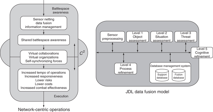
FIGURE 17.1
Network-centric and the Joint Director of Laboratories fusion models.

The fusion model begins with data generation and choosing the right types of sensors or sources (level 0),^‡ providing techniques for detecting and identifying targets of interest (level 1), progressing to the development of situational awareness (level 2) and on to higher levels of human awareness and multilevel feedback. Fundamentally however, the JDL model focuses on a centralized framework, for instance, multiple sensors feeding information to a local fusion processing center to provide a set of local target tracks, and then sending the results to decision managers in that region.

The difficulty with developing fusion techniques for the network enterprise is adopting a mathematical framework that squarely integrates fusion processing directly into the network structure. Directly applying centralized fusion concepts to a distributed network is not the answer. As we see, distributed fusion is concerned with the problem of detecting multiple pathways in the network^§ that share common data. This represents a double counting of information (uncertainty), essentially causing the fusion network to become overconfident. Dr. Chee-Yee Chong described this as the chicken little effect, where, for example, a commander receives confirmation of battlefield conditions from an assumed set of independent sources that in turn used the same upstream source to develop their assessment. Finding and compensating for these common pathways form the primary goal of distributed network fusion.

To show how fusion performance can be affected by a network-centric system, we will build a conceptual network-centric example and develop the corresponding distributed fusion concepts. In doing so, we hope to provide both the fusion community and the network-centric community with an understanding of some of the important concepts, involving distributed fusion.

Figure 17.1 represents one example of how technologies such as fusion are portrayed within the network-centric literature (Ref. 1, p. 89, in part), and fusion as it is often presented in the fusion literature (JDL fusion model). Network-centric system designers have focused on developing the network framework, while assuming that key technologies such as fusion could be easily inserted into the network structure as one of many higher-level processing techniques. Although the JDL model is applicable to a network-centric system, the literature has focused its use on centralized architectures. When dealing with distributed networks, an additional level of complexity is necessary.

We will examine this level of complexity through a sample network-centric system, and in doing so we will provide some insight into how fusion information is passed throughout the network.

The structure of this chapter is as follows. In Section 17.2, we provide a sample network-centric system, involving multiple sensing platforms, each platform concerned with generating locally fused track estimates of targets in their field-of-view and sending the results to be fused globally (e.g., the ground station) with track estimates generated by other local platforms within the network. From this network layout, we develop the corresponding fusion network and use it as an example for the rest of the chapter. Section 17.3 describes the concepts of the information graph. This approach is a convenient method for locating common pathways that affect overall fusion performance. Section 17.4 describes the general fusion concepts used to eliminate redundant information along these common network paths and conditional independence—a concept necessary to understand the fusion techniques that follow. Section 17.5 discusses five common network fusion techniques. The first four techniques rely on the assumption of conditional independence in addressing how each approach treats the two fundamental sources of distributed network error—common process noise and common priors. The fifth technique assumes covariance consistency between track uncertainties, and as such is not based on conditional independence. Finally, Section 17.6 provides an example of fusion performance. We focus on only one aspect of network fusion—the hierarchical fusion architecture. Hierarchical fusion is more common than one would expect and the results are representative of performance issues that occur in many of the network structures.

It is hoped that this chapter will provide both network-centric developers and fusion developers with an understanding of the additional complexities that distributed fusion requires to function within the network-centric environment.

17.2 Distributed Fusion within a Network-Centric Environment

Within the military, complex network-centric operations can be seen at many levels of operation—tactical and strategic. At the tactical level, airborne platforms process measurements from onboard (organic) or nearby sensors to create ground target track estimates (local fusion) of target activity in the local region. These estimates can be fused with similar track estimates from other platforms to form global estimates of overall target activity (global fusion) in the region. In turn, these global estimates may also be sent to higher process or command centers, which may focus on developing an overall estimate of battlefield activity.

These concepts provide the basis for developing an interrelated system of sensors, communication networks, local processing platforms (e.g., aircraft, ground stations), and regional processing centers that integrate and fuse track state estimates and uncertainties from a wide range of sources over a complex information grid used by local battlefield command and higher headquarter centers that could be located halfway around the globe. Network-centric operations provide the means to transform military operations from sets of stovepiped systems that collect data independently into a tightly integrated distribution of information flow. This involves operating conditions that may be hampered by communication bandwidth limits and fixed but differing data structures that, in some cases, limit the quality of information passed. For instance, an unattended ground-based set of acoustic sensors may send target measurements to a local control node within its sensor array, constrained by processing speeds, operating battery life, and communication update rates. These units cannot afford to process and transmit updates at regular intervals or to maintain a database of full track pedigree (track history). Rather, they may send current local track estimates asynchronously to some downstream processing center (e.g., local aircraft) that would take on the role of more elaborate track processing.

Figure 17.2 shows a sample network-centric operation along with the corresponding fusion network. This example will be the basis of our discussions in this chapter. Each of the subsystems—aircraft, acoustic sensor suite, the ground station, and the communication links—will provide the backdrop for decomposing this sample network system into network components that formulate distributed fusion elements. In this case, the illustrated structure initially divides the network into two different substructures, involving hierarchical fusion with and without feedback. More specifically, airborne platforms A and B independently compute (fuse) dynamic track estimates from onboard (organic) sensors. These fused local track state estimates and the corresponding covariance uncertainty errors (F_A and F_B, respectively) are transmitted to a ground station, E, which fuses the results globally (F_E). The ground station is assumed to transmit a refinement of individual track estimates (reduced fused covariance errors) back to each platform. This example of hierarchical fusion with feedback is shown by the corresponding fusion network on the right. The dual path (double arrows) indicates feedback of the fused global results to each local platform.

Images

FIGURE 17.2
Comparison of a simplified tactical network-centric system and the corresponding fusion network.

The second case involves platforms C and D. In this case, a transmitting node from a set of acoustic sensors (D) feeds local track estimates (F_D) directly to the airborne platform (C), which in turn, fuses these estimates with onboard sensor measurements (F_C). The combined fused tracks are sent to a ground station for further processing (F_E), but the global fused error estimates are not sent back to the local platforms. This case represents hierarchical fusion without feedback.

Other less obvious network examples include, for instance, platform A, where sensors S₁ and S₂ feed F_A. This is an example of centralized fusion—track estimates are formed from the sensors directly on board the platform. Note that hierarchical fusion appears to be similar to centralized fusion but involves multiple stages of track processing. For the fully distributed fusion network, we emphasize sharing fused track estimates directly between each of the three nodes (i.e., airborne platforms A, B, and C). For instance, each of the platforms could share fused track estimates directly with each other by broadcasting locally fused results (fused network of Figure 17.2 linking F_A, F_B, and F_C directly without the ground station).

The fundamental types of fusion architectures are shown in Figure 17.3. Centralized fusion is relatively straightforward, taking in raw measurements directly from the sensors. We usually assume that each sensor generates its own target reports (measurements) independently. Data are collected on a particular target from each sensor; sensor data streams are aligned spatially and temporally, and sensor reports associated with the target are used to formulate a single fused track estimate. The track estimate becomes more refined as more measurements are received.

Within a hierarchical architecture, track results are generated at local fusion processing nodes (centralized architecture), and track estimates are sent in turn to higher nodes (global fusion nodes) to generate a common track estimate. Hierarchical fusion takes advantage of the diversity between local nodes such as the diversity of different sets of sensors to view the target, maintaining local storage of assigned sensor reports and track histories at the originating node, while transmitting refined track estimates. Feedback may be used to take advantage of any fused track improvements developed at the higher nodes by redistributing the reduced error uncertainty estimates back to the local fusion nodes. Hierarchical systems may compensate for limited communication bandwidths that restrict the quantity (and quality) of data from local nodes. Hierarchical formats can ensure considerable communication savings.

Images

FIGURE 17.3
Traditional network fusion architectures.

Distributed architectures do not assume superior or subordinate roles between nodes; we can think of this approach as passing information between equals. Data sharing is based on the needs of each node—requesting information from other platforms to help reduce local track uncertainty error or passing results only at opportune times. In the first case, an aircraft may take advantage of well-placed geometries of other aircrafts to reduce track error or extend track continuity because of local terrain obscuration. In fact, with the advent of agent technology and the knowledge of platform locations, a single platform could improve local estimates by adapting agent techniques to search out and test optimal platform geometries before requesting or even fusing the results from local estimates. In the second case, track results may be transmitted only when track estimates have changed significantly.

Network-centric systems add an additional level of complexity to fusion processing. In the past, as long as we operated within centralized fusion framework, processing raw sensor measurements or working with track estimates updated each time new data were received (full-communication rate), the results were easy to deal with and mathematically optimal. However, treatment of track estimates within a network-centric system involves inherently redundant path links between nodes. Regardless of the architecture, these redundancies must be found and the common correlated estimation errors removed before they corrupt subsequent processing. There are two types of common errors to consider: prior estimates and process noise. The complexity of the architecture determines how and where these errors are generated. The fusion process determines how they are removed.

As such, distributed fusion processing should consider three factors: the network architecture, communication links within the network, and applicable fusion algorithms.

Architectures. The network architecture focuses on the node structure between the sensors and the eventual user. The primary architectures considered may involve any combination of centralized, hierarchical (with and without feedback), or distributed fusion. Centralized architectures transmit sensor generated raw measurements directly to a common fusion node. These architectures² provide local stovepiped processing centers that limit network-centric development. Any number of fusion texts that discuss this approach can be found.^{5, 6, 7, 8, 9 and 10}

Hierarchical architectures fuse global track estimates from some combination of local fusion processing nodes, forming a subordinate–superior relationship. That is, centralized fusion nodes provide local fused estimates from one or more sensors and send the results to a common command node to develop a global fused track estimate. Hierarchical nodes can involve feedback to reduce local track covariance errors.

Distributed fusion extends the concepts of hierarchical fusion to more general conditions. Under this form, there is no subordinate–superior nodal relationship. Each node can communicate estimates to other nodes as needed and in turn receives estimates.

Communications. Communication in connectivity plays a critical role within a network-centric framework. How each node is connected determines the applicability, performance, and utility of the fusion algorithm. Connectivity pathways and bandwidth constraints determine whether nodes can accept large amounts of raw data or smoothed track estimates are needed. These constraints affect how path links are formed and determine whether full rate or intermediate transmissions are used. Full-rate communication ensures performance optimality by creating in essence supermeasurements but may not be practical under realistic operational settings. Creating hierarchical processing nodes and transmitting track estimates can reduce bandwidth requirements but adds more decision processing layers. Information push or pull dictates the need and complexity of feedback.

Fusion algorithm. Choice of fusion algorithm is based on the network architecture, communication constraints, node processing capabilities and limits, and command and processing protocols. The network structure and operational needs create path link redundancies affected by common track errors: process noise (target dynamics) and prior estimates (fusion with previously communicated track estimates). Choosing the right fusion algorithm is based on the need to minimize these errors. For instance, if target dynamics is considered well-behaved (e.g., tracks generated within predetermined shipping lanes), process noise can probably be ignored. Each fusion algorithm discussed treats these errors differently. Depending on how these assumptions match real-world conditions determines how well the fusion algorithm will perform.

Images

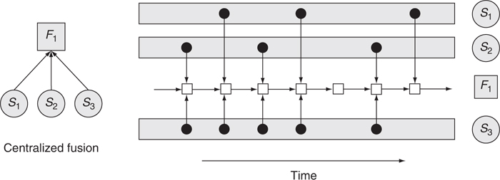
FIGURE 17.4
Information graph for the centralized fusion architecture.

We address how these factors impact network-centric operations. However, first we need to introduce the concepts of the information graph and how it can be used to locate common node links (fusion double counting) within a system network.

17.3 Information Graph

The information graph is a convenient means to understand how fusion process flows impact a network system. In this section we look at the information graph for the fusion architectures in Figure 17.3, based on our network example. Examining these graphs gives us an insight into how fusion is affected by the network system.*

17.3.1 Centralized Architecture

The centralized architecture gives the simplest information graph (Figure 17.4). Each sensor provides an independent set of measurements that is processed at a local fusion node, F₁, to develop and update a common set of track estimates. Updates may be at an asynchronous or synchronous rate. The shaded rectangular boxes (on the right side of the figure) represent measurements generated by each sensor over time. Note that fusion updating can take place even when there are no measurements. Track state estimates are generated directly from the sensor’s raw measurements. As such, fused track state estimates are considered optimal.

Referring back to the network-centric architecture in Figure 17.2, each airborne platform and the acoustic network represent examples of centralized architectures. Such systems drove the development of fusion research in the early years that led to the formulation of the multitiered JDL fusion model (Figure 17.1).

However, as these systems began to share results across the network, the network complexity began to contribute to additional problems.

17.3.2 Hierarchical Architecture without Feedback

Hierarchical fusion represents the next level of complexity within a network structure. As Figure 17.5 shows, local centralized nodes (F₁ and F₂ representing the aircraft platforms in Figure 17.2) transmit fused target state estimates and track covariance errors to the regional global fusion node, F₃ (e.g., the ground station). The hierarchical architecture on the left side of Figure 17.5 appears to be a natural extension of the centralized approach. However, the information graph (on the right) shows a more complex underlying structure—redundant data pathways feed the global fusion node over time. The figure shows two such pathways by following the two broad-lined paths starting in F₁ at point A and terminating at point E in the fusion center F₃. Track estimates are generated at point A sent to the fusion node F₃ at point B and continue to be processed locally within F₁ over time. At point C, these estimates are updated and once again sent to F₃ at point E. Similarly the fusion center updates its own track estimates from point B at point D. However, when the estimates from F₁ (point C) are fused with the results from point D at point E, this could lead to a smaller fused error due to the common uncertainty originally presented at point A and sent along these two paths. This results in an overconfident global estimate usually much smaller than it should be. Because the information is not mutually exclusive, this redundant information occurs each time a local node sends new updates but continues to process the same error. This could lead to track loss because the redundancy could contribute to an overall track error much smaller than that is reasonable for the target dynamics.

Images

FIGURE 17.5
Information graph for the hierarchical fusion architecture without feedback.

Images

FIGURE 17.6
Multitiered hierarchical fusion flow for the network-centric acoustic sensor flow.

The local nodes (e.g., point A) represent the source of common error that needs to be accounted for and removed each time the fusion center receives a new update. The information graph provides a natural means of determining when and where these redundant pathways are created.

Referring back to Figure 17.5, we can now formulate where these common pathways occur, by finding the common ancestors in the system. For example, the common ancestor originates at the local aircraft nodes, F_A and F_B, when no feedback is used.

Similarly nodes F_C and F_D represent another form of hierarchical fusion without feedback. Tracks are generated at F_D from local acoustic sensors and sent to the aircraft to fuse with track updates processed at F_C. The combined tracks are sent to the ground station. This process will be similar to the multitiered hierarchical flow shown in Figure 17.6, where the sensor inputs have been dropped for simplicity.

17.3.3 Hierarchical Architecture with Feedback

Much of the previous discussion involving hierarchical fusion without feedback is applicable to hierarchical fusion involving feedback. Referring to Figure 17.7, the main difference is that when information is sent back to the local nodes, the common source of error now becomes the higher (global) fusion node, F₃. In this case, the global node generates combined target estimates based on both the local fusion platforms and from any organic sensors. This redundant information, formed at the global fusion center, must be removed before the results are sent back to the individual platforms to reduce local track errors. The advantage of this approach is that the local nodes (F₁ and F₂) will operate with nearly identical uncertainty errors to those at the global fusion node, F₃, essentially improving overall track processing for each local track. The disadvantage is that if the common information in the global estimate is not removed, then it is more difficult for the overall system to recover. That is, the fused global error becomes so small that it is difficult to associate subsequent updates with the same track.

Referring to the information graph in Figure 17.7, note that the fused estimates generated at point A in F₃ are sent back to the lower-level platform, F₁ (at point B), where they are subsequently fused with the current local track state, then updated to the current time at point D. Thus the source of redundancy (common predecessor) for fusion with feedback architectures resides with the fusion center.

Images

FIGURE 17.7
Information graph for the hierarchical fusion architecture with feedback.

17.3.4 Distributed Architecture

Distributed fusion represents the next level of fusion complexity in a network-centric system. Hierarchical fusion is the simplest form of distributed fusion architectures, and its theoretical development forms the basis for developing more complex distributed fusion systems. As we saw with the two feedback cases of hierarchical fusion, distributed fusion is highly dependent on the architecture and the communication protocol to locate and eliminate the common information sources. Complex architectures, such as cyclic communications, contain multiple common predecessor nodes that form multiple redundant paths, much earlier in the process.^11,21,22

Broadcast networks are the simplest form of distributed fusion (Figure 17.8) that easily demonstrates network flow redundancy. Assume that after each local fused update, the track estimates are transmitted directly to the other fusion nodes (e.g., F₁ transmits simultaneously to F₂ and F₃). Then path redundancy originating at point A (in this example) must be removed from the fused estimates at points C and D before it is retransmitted back at point E.

To see a distributed network within the network-centric operation in Figure 17.2, it would be as if we removed the ground station and allowed each of the three airborne platforms to broadcast fused track results to each other. Transmissions need not be synchronous. For example, any form of significant change in the track state could be used to initiate a transmission, or a node may generate a request to all other nodes, when it has to reduce large locally generated covariance errors.

As we noted earlier, a complex network-centric operation, such as that represented in Figure 17.2, usually is composed of any combination of the basic fusion network structures in Figure 17.3. Local nodes represent centralized architectures. Hierarchical conditions exist between local fusion centers and a global fusion center. Extending this concept, one could see regional nodes forming further hierarchies with a battlefield command center, or multiple airborne platforms using local agents to seek out other regional airborne systems to help reduce local track uncertainties when their sensors are inadequate (e.g., distributed fusion). However, complex distributed architectures should be constructed with caution because of the inherent complexity, and the difficulty in finding common sources of error. Only a limited number of simple structured distributed architectures have been studied.* Current research is under way to examine techniques to handle more general networks, such as covariance intersection (CI)²⁷ and genealogy fusion.²⁸

Images

FIGURE 17.8
Information graph for the distributed fusion (broadcast) architecture.

17.4 Fusion Algorithm and Distributed Estimation

Traditional track fusion algorithm development has focused on centralized architectures. These algorithms assume that sensor measurements (reports) are generated independently. Measurement independence is the reason why centralized fusion is theoretically optimal. Distributed fusion researchers have recognized that fusion across a network environment adds an additional level of complexity to standard centralized fusion approaches. This added complexity is driven by the impact of common process noise and common priors. This section lays the foundation for this process.

Revisiting the hierarchical fusion format in Figure 17.5, assume two local nodes are tracking the same target based on individual discrete-time dynamic models of the form:

\begin{matrix} {\hat{x}}_{F_{i}} (k + 1) & = & F_{F_{i}} (k) {\hat{x}}_{F_{i}} (k) + G_{F_{i}} (k) v (k) \\ P_{F_{i}} (k + 1) & = & F_{F_{i}} (k) P_{F_{i}} (k) F_{F_{i}} (k)' + G_{F_{i}} (k) Q (k) G_{F_{i}} (k)' & (17.1) \\ k & = & 0, 1, 2, ... \end{matrix}

$\begin{matrix} {\hat{x}}_{F_{i}} (k + 1) & = & F_{F_{i}} (k) {\hat{x}}_{F_{i}} (k) + G_{F_{i}} (k) v (k) \\ P_{F_{i}} (k + 1) & = & F_{F_{i}} (k) P_{F_{i}} (k) F_{F_{i}} (k)' + G_{F_{i}} (k) Q (k) G_{F_{i}} (k)' & (17.1) \\ k & = & 0, 1, 2, ... \end{matrix}$

where ${\hat{x}}_{F_{i}} (k)$ ${\hat{x}}_{F_{i}} (k)$ represents the state vector (target location or type) updated over k time updates for node F_i, P_{F_i}(k) is the state transition matrix, and v(k) being a zero-mean white Gaussian process noise with covariance Q(k) and associated covariance error, P_{F_i}(k+1).

For each local node, measurements are received from the sensor mix, modeled as

\begin{matrix} z_{s_{i}, m} (k + 1) = H_{S_{i}} (k) x_{F_{i}} (k) + w_{S_{i}} (k) \\ S_{i} = platform sensor, k = 0, 1, 2, ... & (17.2) \end{matrix}

$\begin{matrix} z_{s_{i}, m} (k + 1) = H_{S_{i}} (k) x_{F_{i}} (k) + w_{S_{i}} (k) \\ S_{i} = platform sensor, k = 0, 1, 2, ... & (17.2) \end{matrix}$

where H_{S_i} is the transition from the state and the measurement, and W_{S_i}(k) represents zero-mean white Gaussian measurement noise with covariance R_{S_i}(k). Measurement history from each sensor can be represented by (see Figure 17.5)

\begin{matrix} S_{1} : Z_{11} = (z_{11}, z_{12}, z_{13}, ...) * & and & S_{2} : Z_{12} = (z_{21}, z_{22}, z_{23}, ...) & for node F_{1} \\ S_{3} : Z_{23} = (z_{31}, z_{32}, z_{33}, ...) & and & S_{4} : Z_{24} = (z_{41}, z_{42}, z_{43}, ...) & for node F_{2} \end{matrix}

$\begin{matrix} S_{1} : Z_{11} = (z_{11}, z_{12}, z_{13}, ...) * & and & S_{2} : Z_{12} = (z_{21}, z_{22}, z_{23}, ...) & for node F_{1} \\ S_{3} : Z_{23} = (z_{31}, z_{32}, z_{33}, ...) & and & S_{4} : Z_{24} = (z_{41}, z_{42}, z_{43}, ...) & for node F_{2} \end{matrix}$

Assume that each platform develops a track estimate based on Kalman filter principles. The local track estimates and covariance matrices are transmitted to the fusion center (e.g., ground station, F₃) to develop a global track state estimate of target position and error covariance, $\hat{x}$ $\hat{x}$ and $\hat{P}$ $\hat{P}$ . The fusion center maintains these estimates along with previous fused updates (priors) from earlier local track transmissions and extrapolated to the current time. These priors are represented by $\bar{x}$ $\bar{x}$ and $\bar{P}$ $\bar{P}$ . Additionally, let x and P represent the true target dynamics.

As each sensor observes the target, a local fused state estimate is formed independently (at nodes F₁ and F₂) and sent to the global fusion center, F₃, to build a common dynamic state estimate of target motion. In other words, a fused global target state estimate is generated on the basis of an assumption of conditional independence between the estimates of F₁ and F₂. To understand this process, let us examine the track state information, generated at each local node. Since the sensor measurements represent the total information present, their collected set can be written as the union of their measurements (e.g., for F₁): Z₁ = Z₁₁ ∪ Z₁₂ = (z₁₁, z₁₂, z₁₃, …) ∪ (z₂₁, z₂₂, z₂₃, …). Similarly Z₂ = Z₂₃ ∪ Z₂₄ for fusion node F₂. These measurement sets contain common information that needs to be removed at F₃.

Figure 17.9^21,22 provides a conceptual framework. We use Z_i/Z_j to represent those measurements in Z_i that are not common to Z_j. Then it is easily shown²¹ that

Z₁∪Z₂ = (Z₁/Z₂)∪(Z₂/Z₁)∪(Z₁∩Z₂)

The conditional independence assumption implies the following:

p (Z_{1} \cup Z_{2} | x) = \frac{p (Z_{1} | x) p (Z_{2} | x)}{p (Z_{1} \cap Z_{2} | x)}

$p (Z_{1} \cup Z_{2} | x) = \frac{p (Z_{1} | x) p (Z_{2} | x)}{p (Z_{1} \cap Z_{2} | x)}$

Images

FIGURE 17.9
Conditional relationship between two nodes to be fused.

This leads to a formulation for the common information by the conditional relation:*

\begin{matrix} p (x | Z_{1} \cup Z_{2}) = C^{- 1} \frac{p (x | Z_{1}) p (x | Z_{2})}{p (x | Z_{1} \cap Z_{2})} & (17.3) \end{matrix}

$\begin{matrix} p (x | Z_{1} \cup Z_{2}) = C^{- 1} \frac{p (x | Z_{1}) p (x | Z_{2})}{p (x | Z_{1} \cap Z_{2})} & (17.3) \end{matrix}$

Here, p(x|Z₁) and p(x|Z₂) are the estimates from local nodes F₁ and F₂, respectively. The common information between the nodes is given in the denominator by p(x|Z₁ ∩ Z₂), which is equivalent to “subtracting out” the common information. The globally fused (joint) information is represented by p(x|Z₁ ∪ Z₂). C is the normalization constant.

For the hierarchical fusion architecture without feedback in Figure 17.5, Equation 17.3 can be adapted to show the common ancestor generated by F₁:

\begin{matrix} p (x | Z_{F_{3}} (E)) = C^{- 1} \frac{p (x | Z_{F_{1}} (C)) p (x | Z_{F_{3}} (D))}{p (x | Z_{F_{1}} (A))} & (17.4) \end{matrix}

$\begin{matrix} p (x | Z_{F_{3}} (E)) = C^{- 1} \frac{p (x | Z_{F_{1}} (C)) p (x | Z_{F_{3}} (D))}{p (x | Z_{F_{1}} (A))} & (17.4) \end{matrix}$

where the redundant information from p(x|Z_F1(A)) is removed.

Similarly, for the hierarchical fusion architecture with feedback in Figure 17.7, we show the common ancestor to be at the global fusion node F₃:

\begin{matrix} p (x | Z_{F_{3}} (E)) = C^{- 1} \frac{p (x | Z_{F_{3}} (C)) p (x | Z_{F_{3}} (D))}{p (x | Z_{F_{3}} (A))} & (17.5) \end{matrix}

$\begin{matrix} p (x | Z_{F_{3}} (E)) = C^{- 1} \frac{p (x | Z_{F_{3}} (C)) p (x | Z_{F_{3}} (D))}{p (x | Z_{F_{3}} (A))} & (17.5) \end{matrix}$

For the distributed architecture in Figure 17.8, all nodes are able to accept information. Thus for node F₁ receiving information from all three nodes, Equation 17.3 becomes

\begin{matrix} p (x | Z_{F_{1}} (E)) = C^{- 1} \frac{p (x | Z_{F_{1}} (B)) p (x | Z_{F_{2}} (C)) p (x | Z_{F_{3}} (D))}{p {(x | Z_{F_{1}} (A))}^{2}} & (17.6) \end{matrix}

$\begin{matrix} p (x | Z_{F_{1}} (E)) = C^{- 1} \frac{p (x | Z_{F_{1}} (B)) p (x | Z_{F_{2}} (C)) p (x | Z_{F_{3}} (D))}{p {(x | Z_{F_{1}} (A))}^{2}} & (17.6) \end{matrix}$

Note that the common information from A was sent to both nodes B and C and as such is taken out twice (the squared term in the denominator). As discussed previously, two sources of error form the basis for reduced track accuracy at the global fusion center: common process noise and common prior errors. When multiple sources develop track estimates on the basis of the same dynamic model, they develop common estimation errors on the target, although the sensor measurements are independent. Thus, the local dynamic model developed for each local source creates a common estimate of the target motion. This cross-covariance matrix defines the error correlation (common process noise) between the sensor tracks generated between the two local sites and gives rise to a fused global covariance matrix, $P = [\begin{matrix} P_{i} & P_{i j} \\ P_{j i} & P_{j} \end{matrix}]$ $P = [\begin{matrix} P_{i} & P_{i j} \\ P_{j i} & P_{j} \end{matrix}]$ , where P_i and P_j are the local covariance matrices for F_i and F_j, respectively; P_ij and P_ji represent the cross-covariance between the local track estimates; that is, P_ij is the cross-covariance between ${\hat{x}}_{F_{i}} (k)$ ${\hat{x}}_{F_{i}} (k)$ and ${\hat{x}}_{F_{j}} (k)$ ${\hat{x}}_{F_{j}} (k)$ , and P_ji between ${\hat{x}}_{F_{j}} (k)$ ${\hat{x}}_{F_{j}} (k)$ and ${\hat{x}}_{F_{i}} (k)$ ${\hat{x}}_{F_{i}} (k)$ . (Henceforth for convenience, we will refer to these state estimates as ${\hat{x}}_{i} (k)$ ${\hat{x}}_{i} (k)$ and ${\hat{x}}_{j} (k)$ ${\hat{x}}_{j} (k)$ , respectively.)

The second source of error between the two local track estimates is on the basis of the common prior information, generated at the global fusion center. As we saw with Figure 17.5, the same covariance error generated at point A was used to update both the local track F₁ and the global fusion center at point B. This common prior has to be removed at the next update at point E.

The next section addresses the development of five different fusion algorithms; each designed to treat these sources of error differently.

17.5 Distributed Fusion Algorithms

There are four types of distributed fusion algorithms that are designed to address the issue of common process noise and common prior errors. These methods assume conditional independence * of the state covariance between the local fusion nodes. They are naïve fusion, cross-covariance fusion, information fusion, and maximum a posteriori (MAP) fusion. A fifth fusion algorithm that focuses on covariance consistency is called covariance intersection (CI).^† This type of approach does not require the conditional independence assumption. Each algorithm treats correlation errors differently. To compare each approach, we will base our discussion on hierarchical fusion without feedback and assume a linear Gaussian formulation. Equations 17.3, 17.4, 17.5 and 17.6, discussed in Section 17.4, are general and apply to either linear or nonlinear conditions. To adapt the following fusion techniques for a particular architecture, we need only to follow a similar approach to develop the equations, as we did with Equations 17.4, 17.5 and 17.6. A detailed discussion of the algorithms^{15, 16, 17, 18, 19, 20, 21, 22, 23, 24, 25 and 26,29} and a historical perspective¹⁶ of this work can be found in the literature. For instance, variations of this work are presented by Li et al.³⁰ and Drummond.³¹ Recently a new work by Zhu³² presents a generalized fusion framework to examine statistical dependency between sensors. This material is not within the scope of this paper and will not be discussed.

17.5.1 Naïve Fusion

Naïve fusion assumes that both common process noise (cross-covariance error) and common priors are negligible. This fusion approach represents the simplest of the four types and it is suboptimal. As such, this approach is better suited for simple tracking problems. This involves track motion under relatively benign tracking conditions (single isolated targets with little ambiguity about the dynamic model). Its simplicity involves minimal computational processing.

The global fused state estimation and corresponding covariance error are shown as

\begin{matrix} \hat{x} = P (P_{i}^{- 1} {\hat{x}}_{i} + P_{j}^{- 1} {\hat{x}}_{j}) \\ P = {(P_{i}^{- 1} + P_{j}^{- 1})}^{- 1} & (17.7) \end{matrix}

$\begin{matrix} \hat{x} = P (P_{i}^{- 1} {\hat{x}}_{i} + P_{j}^{- 1} {\hat{x}}_{j}) \\ P = {(P_{i}^{- 1} + P_{j}^{- 1})}^{- 1} & (17.7) \end{matrix}$

Note that the fused track covariance is the inverse of the sum of the inverses of the local track covariance matrices. Thus, the fused covariance could have values much smaller than either individual error, which can lead to conditions of overconfidence.*

Because track estimates are generated at each local fusion node separately, a method is needed to link the correct track estimates from both nodes (association). The corresponding performance metric^† provides a basis for assigning the most appropriate individual track estimates to be fused (between local nodes F₁ and F₂ in Figure 17.5):

\begin{matrix} C_{i j} = {| | {\hat{x}}_{i} - {\hat{x}}_{j} | |}_{{(P_{i} + P_{j})}^{- 1}}^{2} & (17.8) \end{matrix}

$\begin{matrix} C_{i j} = {| | {\hat{x}}_{i} - {\hat{x}}_{j} | |}_{{(P_{i} + P_{j})}^{- 1}}^{2} & (17.8) \end{matrix}$

This metric represents the Mahalanobis distance metric, commonly used within Kalman filter tracking.

17.5.2 Cross-Covariance Fusion

Cross-covariance fusion takes into account common process noise but assumes all common priors are negligible. The fusion algorithm is represented as follows:

\begin{matrix} {\begin{matrix} \hat{x} = {\hat{x}}_{i} + (P_{i} - P_{i j}) (P_{i} + P_{j} - P_{i j} - P_{j i}) \end{matrix}}^{- 1} ({\hat{x}}_{j} - {\hat{x}}_{i}) \\ P = {P_{i} - (P_{i} - P_{i j}) (P_{i} + P_{j} - P_{i j} - P_{j i})}^{- 1} (P_{i} - P_{j i}) & (17.9) \end{matrix}

$\begin{matrix} {\begin{matrix} \hat{x} = {\hat{x}}_{i} + (P_{i} - P_{i j}) (P_{i} + P_{j} - P_{i j} - P_{j i}) \end{matrix}}^{- 1} ({\hat{x}}_{j} - {\hat{x}}_{i}) \\ P = {P_{i} - (P_{i} - P_{i j}) (P_{i} + P_{j} - P_{i j} - P_{j i})}^{- 1} (P_{i} - P_{j i}) & (17.9) \end{matrix}$

Cross-covariance fusion requires more information to be communicated because of the cross-covariance terms, P_ij and P_ji (between ${\hat{x}}_{i}$ ${\hat{x}}_{i}$ and ${\hat{x}}_{j}$ ${\hat{x}}_{j}$ ).^‡ These results are optimal only within a maximum likelihood sense.¹⁹ Cross-covariance fusion may be applicable under conditions where a target is known to exist (e.g., low background clutter) and tracking parameters need to be determined. Note that when P_ij = P_ji = 0, this form is simply the naïve fusion rule.^§

The corresponding metric is given by the χ² test:

\begin{matrix} C_{i j} = {| | {\hat{x}}_{i} - {\hat{x}}_{j} | |}_{{(P_{i} + P_{j} - P_{i j} - P_{j i})}^{- 1}}^{2} & (17.10) \end{matrix}

$\begin{matrix} C_{i j} = {| | {\hat{x}}_{i} - {\hat{x}}_{j} | |}_{{(P_{i} + P_{j} - P_{i j} - P_{j i})}^{- 1}}^{2} & (17.10) \end{matrix}$

providing a “polynomial goodness of fit” to the dynamic model.

17.5.3 Information Matrix Fusion

Information fusion assumes that the common prior is dominant, and common process noise is negligible. The fusion algorithm is represented as follows:

\begin{matrix} \hat{x} = P (P_{i}^{- 1} {\hat{x}}_{i} + P_{j}^{- 1} {\hat{x}}_{j} - {\bar{P}}^{- 1} \bar{x}) \\ {\begin{matrix} P = (P_{i}^{- 1} + P_{j}^{- 1} - {\bar{P}}^{- 1}) \end{matrix}}^{- 1} & (17.11) \end{matrix}

$\begin{matrix} \hat{x} = P (P_{i}^{- 1} {\hat{x}}_{i} + P_{j}^{- 1} {\hat{x}}_{j} - {\bar{P}}^{- 1} \bar{x}) \\ {\begin{matrix} P = (P_{i}^{- 1} + P_{j}^{- 1} - {\bar{P}}^{- 1}) \end{matrix}}^{- 1} & (17.11) \end{matrix}$

The common prior (point B in Figure 17.5) represents the cumulative history of the global fused track estimate and covariance error. This includes extrapolating the fused track (F₃), based on the track pedigree and all contributions from the local nodes (F₁ and F₂). The common prior information is noted by $\bar{x}$ $\bar{x}$ and $\bar{P}$ $\bar{P}$ .

Information fusion is a natural complement to the information graph. The simplicity of this approach is well suited in a number of ways:

The information fusion approach is only slightly more complicated than naïve fusion. If the common priors were negligible, the information fusion becomes the naïve fusion rule. This is consistent with the assumption that the local estimates are conditionally independent.
There is no need to maintain cross-covariance information between the local nodes. This significantly reduces communication bandwidth requirements.
This approach is optimal when there is no (significant) process noise—the target dynamic model is deterministic, or each local update is transmitted to the fusion center at each update (full-rate communications).
Information fusion is applicable when target dynamic modeling errors can be quickly established, such as detecting maneuvers quickly and assigning the appropriate target model (e.g., using multiple-filter models).

The corresponding metric is as follows:

\begin{matrix} C_{i j} = {| | \hat{x} - {\hat{x}}_{i} | |}_{{(P_{i})}^{- 1}}^{2} + {| | \hat{x} - {\hat{x}}_{j} | |}_{{(P_{j})}^{- 1}}^{2} - {| | \hat{x} - \bar{x} | |}_{{(\bar{P})}^{- 1}}^{2} & (17.12) \end{matrix}

$\begin{matrix} C_{i j} = {| | \hat{x} - {\hat{x}}_{i} | |}_{{(P_{i})}^{- 1}}^{2} + {| | \hat{x} - {\hat{x}}_{j} | |}_{{(P_{j})}^{- 1}}^{2} - {| | \hat{x} - \bar{x} | |}_{{(\bar{P})}^{- 1}}^{2} & (17.12) \end{matrix}$

17.5.4 Maximum A Posteriori Fusion

MAP fusion represents the most complete but also the most complex form of fusion. MAP fusion incorporates the effects of the common prior and common process noise. The fusion algorithm is represented as follows:

\begin{matrix} \hat{\begin{matrix} x \end{matrix}} = \bar{x} + W_{i} ({\hat{x}}_{i} - \bar{x}) + W_{j} ({\hat{x}}_{j} - \bar{x}) \\ P = \bar{P} - \sum_{x \hat{z}} \sum_{\hat{z} \hat{z}}^{- 1} \sum_{\hat{z} x}^{'} & (17.13) \end{matrix}

$\begin{matrix} \hat{\begin{matrix} x \end{matrix}} = \bar{x} + W_{i} ({\hat{x}}_{i} - \bar{x}) + W_{j} ({\hat{x}}_{j} - \bar{x}) \\ P = \bar{P} - \sum_{x \hat{z}} \sum_{\hat{z} \hat{z}}^{- 1} \sum_{\hat{z} x}^{'} & (17.13) \end{matrix}$

where

\begin{matrix} [W_{i} W_{j}] = \sum_{x \hat{z}} \sum_{\hat{z} \hat{z}}^{- 1} \\ \begin{matrix} \begin{matrix} \begin{matrix} \begin{matrix} \sum_{x \hat{z}} = [\sum_{i} \sum_{j}] \end{matrix} & and \end{matrix} \end{matrix} & \sum_{\hat{z} \hat{z}} \end{matrix} = [\begin{matrix} {\sum^{̂}}_{i i} & {\sum^{̂}}_{i j} \\ {\sum^{̂}}_{j i} & {\sum^{̂}}_{j j} \end{matrix}] & (17.14) \\ \hat{z} = [\begin{matrix} {\hat{x}}_{i}^{'} & {\hat{x}}_{j}^{'} \end{matrix}]' \end{matrix}

$\begin{matrix} [W_{i} W_{j}] = \sum_{x \hat{z}} \sum_{\hat{z} \hat{z}}^{- 1} \\ \begin{matrix} \begin{matrix} \begin{matrix} \begin{matrix} \sum_{x \hat{z}} = [\sum_{i} \sum_{j}] \end{matrix} & and \end{matrix} \end{matrix} & \sum_{\hat{z} \hat{z}} \end{matrix} = [\begin{matrix} {\sum^{̂}}_{i i} & {\sum^{̂}}_{i j} \\ {\sum^{̂}}_{j i} & {\sum^{̂}}_{j j} \end{matrix}] & (17.14) \\ \hat{z} = [\begin{matrix} {\hat{x}}_{i}^{'} & {\hat{x}}_{j}^{'} \end{matrix}]' \end{matrix}$

The coefficients, $W_{k | k} = [\begin{matrix} W_{i} & W_{j} \end{matrix}] = \begin{matrix} \sum_{x \hat{z}} & \sum_{\hat{z} \hat{z}}^{- 1} \end{matrix}$ $W_{k | k} = [\begin{matrix} W_{i} & W_{j} \end{matrix}] = \begin{matrix} \sum_{x \hat{z}} & \sum_{\hat{z} \hat{z}}^{- 1} \end{matrix}$ , form the gain matrices that determine the effective contribution from each local node. $\sum_{x \hat{z}} = [\sum_{1} \sum_{2}]$ $\sum_{x \hat{z}} = [\sum_{1} \sum_{2}]$ represents the cross-covariance between the target state x and the joint local estimates, $\hat{z} = [\begin{matrix} {\hat{x}}_{i}^{'} \\ {\hat{x}}_{i}^{'} \end{matrix}]$ $\hat{z} = [\begin{matrix} {\hat{x}}_{i}^{'} \\ {\hat{x}}_{i}^{'} \end{matrix}]$ , for nodes F₁ and F₂ (Figure 17.5). Additionally, $\sum_{\hat{z} \hat{z}} = [\begin{matrix} {\sum^{̂}}_{i i} & {\sum^{̂}}_{i j} \\ {\sum^{̂}}_{j i} & {\sum^{̂}}_{j j} \end{matrix}]$ $\sum_{\hat{z} \hat{z}} = [\begin{matrix} {\sum^{̂}}_{i i} & {\sum^{̂}}_{i j} \\ {\sum^{̂}}_{j i} & {\sum^{̂}}_{j j} \end{matrix}]$ is the covariance matrix of $\hat{z}$ $\hat{z}$ .

This approach deviates from the information fusion algorithm. MAP fusion provides the best linear minimum mean squared error (LMMSE) estimate, when the local state estimates operate under non-Gaussian assumptions, and we assume that the target is static or communication is of full rate (e.g., communicate the updated state estimates after each sensor observation). For less than full-rate communication, MAP may become suboptimal.* Much of the literature focuses on the static condition and therefore the impact of multiple iterations on MAP performance has not been fully studied.²⁶

An application of MAP performance would involve conditions where there is a potential for track maneuvering with significant deviation in local track performance. The primary disadvantage of MAP processing is the complexity of the fusion equations. Note that when $\sum_{i j} = \sum_{i i} {\sum^{¯}}^{- 1} \sum_{j j}$ $\sum_{i j} = \sum_{i i} {\sum^{¯}}^{- 1} \sum_{j j}$ (correlation is affected only by the common prior), the MAP fusion process reverts to the information filter.

To summarize, the four fusion rules treat track performance on the basis of their consideration of common process noise and common prior information. Naïve fusion ignores the effects of both sources of error. Cross-covariance fusion is concerned only with common process noise, whereas information fusion is concerned with common priors. Finally MAP fusion accommodates both sources of error.

With the advent of adaptive multiple model fusion algorithms of the four cases, the information fusion process provides the best choice in general.

17.5.5 Covariance Intersection (CI) Fusion

CI deviates from the precepts of the four fusion algorithms, discussed in Sections 17.5.1, 17.5.2, 17.5.3 and 17.5.4, by not making any claim of conditional independence between the local track estimates.^27,33 The developers of CI recognize that local estimates are correlated. However their basic premise is that conditional independence is “an extremely rare property” and relying on this condition is not a viable means of developing robust track estimate approximations to the centralized case.²⁷ Each local track covariance must be artificially increased to maintain the assumption of correlation at the fusion node. Researchers continue to debate the merits of CI against that of the other approaches, such as information fusion.

The fundamental nature of CI relies on a geometric interpretation of the Kalman filter. The motivation of this approach gives a conservative estimate whenever correlation between ${\hat{x}}_{1}$ ${\hat{x}}_{1}$ and ${\hat{x}}_{2}$ ${\hat{x}}_{2}$ is unknown. Under these conditions, the optimal fusion algorithm may be computationally infeasible but can be shown to be bounded by the CI covariance estimate, P_CI.³³

The CI fusion algorithm is given by

\begin{matrix} {\hat{x}}_{CI} = P_{CI} [ω P_{i}^{- 1} \hat{x} + (1 - ω) P_{j}^{- 1} {\hat{x}}_{j}] \\ P_{CI} = {[ω P_{i}^{- 1} + (1 - ω) P_{j}^{- 1}]}^{- 1} & (17.15) \end{matrix}

$\begin{matrix} {\hat{x}}_{CI} = P_{CI} [ω P_{i}^{- 1} \hat{x} + (1 - ω) P_{j}^{- 1} {\hat{x}}_{j}] \\ P_{CI} = {[ω P_{i}^{- 1} + (1 - ω) P_{j}^{- 1}]}^{- 1} & (17.15) \end{matrix}$

where ω is bounded by a range between [0, 1].

A close examination of ω leads to some interesting results. The CI fusion equation is similar in form to the simple convex combination algorithm (naïve fusion).³³ That is, the naïve covariance matrices for the two local nodes are P_i and P_j and rewritten for CI as ω⁻¹P_i and (1 − ω)⁻¹P_j, respectively, where ω is bounded between [0, 1]. The CI covariance matrices provide a conservative bound compared with the naïve fusion approach. Conceptually, the CI approach can be visualized as a weighted assessment of the two overlapping local covariance estimates. Where the traditional naïve fusion approach would result in a fused covariance estimate smaller than the overlapped region between the two local track covariance regions $(P_{i}^{- 1} + P_{j}^{- 1})$ $(P_{i}^{- 1} + P_{j}^{- 1})$ , CI subsumes the overlapped area, attributing a higher uncertainty to the local track and having a lower weighted value of ω. For example, if the covariance error for node F₁ has a weighting ω of 0.1, P_CI results would be dominated by the uncertainty in F₁, incorporating a fused covariance slightly smaller than P₁ and only a small portion of the error in F₂ (similar in size to the overlapping area). A value of 0.5 for ω would give the same state estimate as in the naïve fusion, but the covariance error would be twice as large:

\begin{matrix} {\hat{x}}_{CI} & = & {\begin{matrix} (P_{1}^{- 1} + P_{2}^{- 1}) \end{matrix}}^{- 1} [P_{1}^{- 1} {\hat{x}}_{1} + P_{2}^{- 1} {\hat{x}}_{2}] = {\hat{x}}_{NF} \\ P_{CI} & = & 2 {(P_{1}^{- 1} + P_{2}^{- 1})}^{- 1} = {2 P}_{NF} & (17.16) \end{matrix}

$\begin{matrix} {\hat{x}}_{CI} & = & {\begin{matrix} (P_{1}^{- 1} + P_{2}^{- 1}) \end{matrix}}^{- 1} [P_{1}^{- 1} {\hat{x}}_{1} + P_{2}^{- 1} {\hat{x}}_{2}] = {\hat{x}}_{NF} \\ P_{CI} & = & 2 {(P_{1}^{- 1} + P_{2}^{- 1})}^{- 1} = {2 P}_{NF} & (17.16) \end{matrix}$

In general, the weight is chosen to minimize either the trace or determinant of P_CI.^27,33

Chong and Mori³³ examine the CI approach from an alternative derivation. They rely on a set-theoretic approach that provides a natural interpretation of the properties of the CI filter. As pointed out, the authors define a tighter bound on the true covariance uncertainty by defining an added weighting factor α² that depends on the estimates to be fused. That is,

\begin{matrix} α^{2} = ({\hat{x}}_{i} - {\hat{x}}_{j})' {[ω^{- 1} P_{i} + {(1 - ω)}^{- 1} P_{j}]}^{- 1} ({\hat{x}}_{i} - {\hat{x}}_{j}) & (17.17) \end{matrix}

$\begin{matrix} α^{2} = ({\hat{x}}_{i} - {\hat{x}}_{j})' {[ω^{- 1} P_{i} + {(1 - ω)}^{- 1} P_{j}]}^{- 1} ({\hat{x}}_{i} - {\hat{x}}_{j}) & (17.17) \end{matrix}$

As long as α² < 1, which is true as long as the two local estimates overlap, the ellipses are accurate representations of the true track uncertainty. Thus Equation 17.15 can be modified as follows:

\begin{matrix} \begin{matrix} {\hat{x}}_{CI} & = & P_{CI} [ω P_{i}^{- 1} {\hat{x}}_{i} + (1 - ω) P_{j}^{- 1} {\hat{x}}_{j}] \\ P_{CI} & = & (1 - α^{2}) [ω P_{i}^{- 1} + (1 - ω) P_{j}^{- 1}] \end{matrix} & (17.18) \end{matrix}

$\begin{matrix} \begin{matrix} {\hat{x}}_{CI} & = & P_{CI} [ω P_{i}^{- 1} {\hat{x}}_{i} + (1 - ω) P_{j}^{- 1} {\hat{x}}_{j}] \\ P_{CI} & = & (1 - α^{2}) [ω P_{i}^{- 1} + (1 - ω) P_{j}^{- 1}] \end{matrix} & (17.18) \end{matrix}$

The key point is that Equation 17.17 can be rewritten into a form similar to the information fusion filter as follows:

\begin{matrix} α^{2} = (ω) {\hat{x}}_{i}^{'} P_{i}^{- 1} {\hat{x}}_{i} + (1 - ω) {\hat{x}}_{j}^{'} P_{j}^{- 1} {\hat{x}}_{j} - {\hat{x}}_{CI}^{'} P_{CI}^{- 1} {\hat{x}}_{CI} & (17.19) \end{matrix}

$\begin{matrix} α^{2} = (ω) {\hat{x}}_{i}^{'} P_{i}^{- 1} {\hat{x}}_{i} + (1 - ω) {\hat{x}}_{j}^{'} P_{j}^{- 1} {\hat{x}}_{j} - {\hat{x}}_{CI}^{'} P_{CI}^{- 1} {\hat{x}}_{CI} & (17.19) \end{matrix}$

As such, α² reassesses a dependency back on the estimates to be fused. The primary difference is that although the estimate lies within the intersection of local covariance errors, there is no probability distribution set to decrease as additional estimates are fused.

We show the equations of each of these approaches in Figure 17.10. Both the original CI and the set-theoretic algorithms are shown. A simple comparison with other fusion approaches can be found in Ref. 33.

Images

FIGURE 17.10
Distributed fusion techniques.

In the next section, we discuss performance comparisons for one of the fusion approaches.* We will restrict ourselves to the hierarchical fusion approach.

17.6 Performance Evaluation between Fusion Techniques

As a core example, we compare performance for the hierarchical fusion architectures. An extended derivation of fusion techniques can be seen in the literature involving closed-form analytic solutions^{23, 24, 25 and 26} and compared analytically.^25,26 The analytic form represents the steady-state fused covariance.

Three forms of the hierarchical fusion approach were used: (1) fusion without feedback (reference Equation 17.4); (2) fusion with feedback (reference Equation 17.5); and (3) fusion with partial feedback (a hybrid of the two).† To ensure consistency between the three approaches, the same track state conditions were used for each fusion technique. The two local nodes are tracking the same target operating under a dynamic model characterized by the discrete-time system discussed in Equations 17.1 and 17.2 and using a Kalman filter to create the local tracks. The scenario involves a single target and two sensor nodes. Each node is tracking the target and providing state estimates to a fusion center following the dynamics of Equations 17.1 and 17.2. In this case, the target dynamics²⁵ are modeled as

x_{k + 1} = [\begin{matrix} 1 & T \\ 0 & 1 \end{matrix}] x_{k} + [\begin{matrix} T^{2} / 2 \\ T \end{matrix}] v_{k}

$x_{k + 1} = [\begin{matrix} 1 & T \\ 0 & 1 \end{matrix}] x_{k} + [\begin{matrix} T^{2} / 2 \\ T \end{matrix}] v_{k}$

The measurements for the two sensors are modeled as follows:

z_{m} = [\begin{matrix} 1 & 0 \end{matrix}] x_{k} + w_{k}

$z_{m} = [\begin{matrix} 1 & 0 \end{matrix}] x_{k} + w_{k}$

where the two measurements are assumed to be independent.

For simplicity, each local sensor delays communicating at fixed update intervals, n, with the fusion center. These intervals can be varied, ranging from full rate to a delay of eight updates (where n ranges from one to eight updates).

The curves generated in Figures 17.11, 17.12 and 17.13 focus on using cross-covariance fusion to provide an upper bound (maximum likelihood—ML) and the information matrix fusion (for n = 1, 2, 4, 8). They were performed using 5000 Monte Carlo simulation trials. Average root-mean-square (RMS) errors were used to estimate the fused covariance values. Each of the graphs represents area ratios for individual track covariance error matrices (uncertainty region) for the fused covariance, A with A*, where A* is the optimal area covered by the steady-state covariance error based on single sensor performance. The comparisons are made over a wide range of track process noise values, q.

Images

FIGURE 17.11
Hierarchical fusion without feedback: error ellipse area ratios with small process noise. (From Chang, K.C., Tian, Z., and Saha, R., IEEE Trans. Aerospace Electr. Syst., 38, 455, 2002. Copyright IEEE 2002.)

Images

FIGURE 17.12
Hierarchical fusion with complete feedback: error ellipse area ratios with variable process noise. (From Chang, K.C., Tian, Z., and Saha, R., IEEE Trans. Aerospace Electr. Syst., 38, 455, 2002. Copyright IEEE 2002.)

The dashed lines represent the analytic results, based on the ML of the cross-covariance (Equation 17.9) and derived in the literature.^{24, 25 and 26} This represents an ideal upper bound to assess overall performance of the hierarchical approach. All remaining performance curves are based on the analytic results^25,26 for various communication rates. These rates show the effect of fused performance when nodes defer communication to the fusion node at fixed intervals. For instance, n = 1 represents full communications (optimal performance) and n = 8 implies that the local nodes wait eight update cycles to communicate to the global (fused) system.

17.6.1 Fusion without Feedback

Fusion without feedback represents a standard command-based hierarchical network structure. Command nodes or battlefield commanders are interested in obtaining the best information possible to plan effective countermeasures, expand surveillance capability by adding complementary sensors to improve observability, or just get the best estimate of track activity. Such curves are ideal in designing distributed fusion systems under a range of process noises, q, and determining acceptable limits regarding communication transmission requirements.

Images

FIGURE 17.13
Hierarchical fusion with partial feedback: error ellipse area ratios with variable process noise. (From Chang, K.C., Tian, Z., and Saha, R., IEEE Trans. Aerospace Electr. Syst., 38, 455, 2002. Copyright IEEE 2002. With permission.)

Figure 17.11 shows that the analytic results are somewhat sensitive to increasing process noise. For higher noise levels, global fusion performance asymptotically approaches steady state at 50%. Under conditions of increasing process noise, reduced communication updates of the local error to the global fusion center cause the performance to approach the upper bounded limits of ML performance. For conditions where we reduce the local updates by eight time updates (n = 8), these errors approach the ML performance bound for relatively small process noise (q = 0.1). Under optimal communication updates (full rate, n = 1), fusion continues to provide improved overall performance. However, the difference between the bounds is not excessive for fusion without feedback, meaning that reasonable delays would not severely impact system performance.

17.6.2 Fusion with Feedback

Much of the discussion in the previous section is also applicable to fusion with feedback. Fusion with feedback is better suited when each of the local nodes needs to maintain the smallest covariance possible—taking advantage of the fused system.

The primary concern with the full feedback approach is the impact of feedback on the state variables not directly observable (velocity and acceleration). These parameters are severely impacted when the process noise becomes too large. As shown in Figure 17.12, fused performance errors significantly deteriorate with increasing process noise and with communication rates less than full rate. When poorly fused results are sent back to the local nodes, local node performance is directly affected, creating an unstable situation (except when full-rate communication occurs, n = 1). In fact, we can see that fusion under these conditions performs worse than the previous “fusion without feedback” case. To compensate for this problem, we examine the effects of partial feedback in the next subsection.

17.6.3 Hierarchical Fusion with Partial Feedback

Partial feedback involves sending only the state estimate without the covariance errors back to the local nodes to contain unstable covariance uncertainties, caused by poorly fused covariance errors. Note that for higher communication intervals, partial feedback performance does degenerate, but the instability problem is reduced and can be controlled sooner. As we will see, this makes partial feedback an effective counter to the full feedback conditions shown earlier.

On the basis of the results in Figure 17.13, we see that the effects of partial feedback in the ratio of the covariance areas provide performance similar to that of hierarchical fusion without feedback.³⁴

17.7 Summary

We have presented the details involving distributed multisensor fusion from a network-centric perspective. Both fusion and network-centric operational research has progressed along parallel paths, with very little interaction. In this chapter, we have attempted to provide a fundamental distributed fusion structure that lays the groundwork for incorporating network fusion principles directly into network-centric systems. Fusion algorithms were presented that address the impact of common sources of tracking and target identification error in a network structure—common process noise and common priors. Additionally, we presented CI fusion, an approach that is not concerned with conditional independence assumption. Examples that relate back to the network-centric structures within a battlefield condition were also presented. Finally, we examined performance examples for analytic solutions for hierarchical fusion under conditions of no feedback, full feedback, and partial feedback. Network-centric applications of distributed fusion can be seen in Refs 35–38 involving multiairborne systems, applications to drug interdiction, enhanced radar management, and wireless ad hoc networks.

References

1. D. Alberts, J. Garstka, F. Stein, Network Centric Warfare, DoD Command and Control Research Program, Library of Congress Cataloging-in-Publication Data, October 2003.

2. Network Centric Warfare: Department of Defense Report to Congress, 31 July 2001.

3. L. Stotts, D. Honey, Gen (R) G. Luck, J. Allen, P. Corpac, Achieving Joint Battle Command in Network Centric Operations, Proceedings of the SPIE, Vol. 5441, pp. 1–12, Orlando, FL, July 2004.

4. Y. LaCerte, B. Rickenbach, Net-centric computing technologies for sensor-to-strike operations, Proceedings of the SPIE, Vol. 5441, pp. 142–150, Orlando, FL, July 2004.

5. E. Waltz, J. Llinas, Multisensor Data Fusion, Artech House, Norwood, MA, 1990.

6. D. Hall, S. McMullen, Mathematical Techniques in Multisensor Data Fusion, 2nd Ed., Artech House, Norwood, MA, USA, 2004.

7. D. Hall, J. Llinas (Eds.) Handbook of Multisensor Data Fusion, CRC Press, New York, NY, 2001.

8. Y. Bar-Shalom, T. E. Fortmann, Tracking and Data Association, Academic Press, Boston, MA, 1988.

9. Y. Bar-Shalom, W. Blair (Eds.) Multitarget-Multisensor Tracking: Applications and Advances, Vol. III, Artech House, Norwood, MA, 2000.

10. S. Blackman, R. Popoli, Design and Analysis of Modern Tracking Systems, Artech House, Norwood, MA, 1999.

11. C. Y. Chong, S. Mori, K. C. Chang, Distributed multitarget multisensor tracking, in Multitarget Multisensor Tracking: Advanced Applications, Y. Bar-Shalom (Ed.) Artech House, Norwood, MA, pp. 247–295, 1990.

12. S. Mori, K. C. Chang, C. Y. Chong, Performance analysis of optimal data association with applications to multiple target tracking, in Multitarget Multisensor Tracking: Applications and Advances, Vol. II, Y. Bar-Shalom (Ed.) Artech House, Norwood, MA, pp. 183–236, 1992.

13. S. Mori, C. Y. Chong, E. Tse, R. Wishner, Tracking and classifying targets without a prior identification, IEEE Transactions on Automatic Control, 31(10), 401–409, 1986.

14. K. C. Chang, C. Y. Chong, Y. Bar-Shalom, Joint probabilistic data association in distributed sensor networks, IEEE Transactions on Automatic Control, 31, 889–897, 1986

15. C. Y. Chong, S. Mori, K. C. Chang, W. Barker, Architectures and algorithms for track association and fusion, Proceedings Second International Conference on Information Fusion, Sunnyvale, USA, pp. 239–246, July 1999.

16. S. Mori, W. Barker, C. Y. Chong, K. C. Chang, Track association and track fusion with non-deterministic target dynamics, IEEE Transactions Aerospace Electronic Systems, 38(2), 659–668, 2002.

17. C. Y. Chong, Hierarchical estimation, in Proceedings of 2nd MIT/ONR C3 Workshop, Monterey, CA, July 1979.

18. C. Y. Chong, Problem characterization in tracking/fusion algorithm evaluation, in Proceedings of the Third International Society of Information Fusion, Fusion, Vol. 1(10), pp. MOC 2/26-MOC/21, Paris, France, 13 July 2000.

19. K. C. Chang, R. Saha, Y. Bar-Shalom, On optimal track-to-track fusion, IEEE Transactions on Aerospace and Electronic Systems, 33(4), 1271–1276, 1997.

20. C. Y. Chong, Distributed architectures for data fusion, in Proceedings First International Conference on Multisource Multisensor Information Fusion ’98, Las Vegas, pp. 85–91, July 1998.

21. C. Y. Chong, S. Mori, Graphical models for nonlinear distributed estimation, 7th International Conference on Information Fusion, Stockholm, Sweden, pp. 614–621, July 2004.

22. M. E. Liggins, II, C. Y. Chong, I. Kadar, M. G. Alford, V. Vannicola, S. Thomopoulos, Distributed fusion architectures and algorithms for target tracking, (Invited paper), in Proceedings of the IEEE, Vol. 85, Issue 1, pp. 95–107, January 1997.

23. K. C. Chang, R. K. Saha, Y. Bar-Shalom, M. Alford, Performance evaluation of multisensor track-to-track fusion, in Proceedings of the 1996 IEEE/SICE/RSJ International Conference on Multisensor Fusion and Integration for Intelligent Systems, pp. 627–631, 1996.

24. K. C. Chang, Z. Tian, R. Saha, Performance evaluation for track fusion with information fusion, in Proceedings First International Conference on Multisource Multisensor Information Fusion ’98, Las Vegas, pp. 648–654, July 1998.

25. K. C. Chang, Evaluating hierarchical track fusion with information matrix filter, in Proceedings of the Third International Society of Information Fusion, Fusion, 00, Paris, France, Vol. 1(10), 13 July 2000.

26. K. C. Chang, S. Mori, Z. Tian, C. Y. Chong, MAP track fusion performance evaluation, in Proceedings of the Fifth International Society of Information Fusion, Annapolis, Vol. 1, pp. 512–519, July 2002.

27. S. Julier, J. Uhlmann, General decentralized data fusion with covariance intersection (CI), in Handbook of Multisensor Data Fusion, D. Hall and J. Llinas (Eds.) CRC Press, New York, NY, 2001.

28. T. Martin, K. C. Chang, A distributed data fusion approach for mobile ad hoc networks, in Proceedings of the Eighth International Conference on Information Fusion (Fusion 2005), Vol. 2(8), pp. 25–28, July 2005.

29. Y. Bar-Shalom, On the track-to-track correlation problem, IEEE Transactions on Automatic Control, 26(2), 571–572, 1981.

30. X. R. Li, Y. Zhu, C. Han, Unified optimal linear estimation fusion—Part I: Unified models and fusion rules, in Proceedings Third International Conference on Information Fusion 00, Vol. 1(10), pp. MOC 2/10-MOC 2/17, Paris, France, 2000.

31. O. E. Drummond, Tracklets and a hybrid fusion with process noise, in Proceedings of SPIE, Signal and Data Processing of Small Targets, Vol. 3163, pp. 512–524, Orlando, FL, 1997.

32. Y. Zhu, Multisensor Decision and Estimation Fusion, Kluwer Academic Publishers, Norwell, MA, 2003.

33. C. Chong, S. Mori, Convex combination and covariance intersection algorithms in distributed fusion, in ISIF Fusion 2001, Montreal Quebec, Canada, August 2001.

34. K. C. Chang, Z. Tian, R. Saha, Performance evaluation of track fusion with information matrix filter, IEEE Transactions on Aerospace Electronic Systems, 38(2), 455–466, 2002.

35. M. Liggins, C. Y. Chong, Distributed multi-platform fusion for enhanced radar management, in 1997 IEEE National Radar Conference, pp. 115–119, 1997.

36. C. Y. Chong, M. Liggins, Fusion technologies for drug interdiction, in Proceedings of the 1994 IEEE Conference on Multisensor Fusion and Integration for Intelligent Systems, pp. 435–441, Las Vegas, October 1994.

37. C. Y. Chong, S. P. Kumar, Sensor networks: Evolution, opportunities, and challenges, in Proceedings of the IEEE, Vol. 91, No. 8, pp. 1247–1256, August 2003.

38. C. Y. Chong, F. Zhao, S. Mori, S. Kumar, Distributed tracking in wireless ad hoc sensor networks, in Proceedings of the 6th International Conference on Information Fusion, pp. 431–438, 2003.

* The author’s affiliation with the MITRE Corporation is provided only for identification purposes and is not intended to convey or imply MITRE’s concurrence with, or support for, the positions, opinions, or viewpoints expressed by the author.

* Knowledgeable entities to enable shared information and collaboration, with an ultimate goal of developing situational awareness.

† JDL represents the first attempt to categorize fusion processing into component technologies. Earlier chapters were devoted to discussing the impact and structure of the JDL model and its role in developing fusion technology.

‡ Sensor preprocessing (not explicitly shown in the figure).

^§ This is only one of the problems for distributed fusion. Others include allocation of processing to different fusion locations, managing communications, etc.

* These concepts are attributed to the work of Chong et al.^{11, 12, 13, 14, 15, 16, 17, 18, 19, 20, 21, 22, 23, 24, 25 and 26} and form the basis for the discussions that follow. Many of the concepts presented are discussed in more detail in these references.

* Other distributed fusion network approaches are discussed in the literature including cyclic, tracklets, and the global restart. Chong et al.¹⁵ discuss these in detail with applicable references given.

* The time index has been removed for simplicity. For instance, S₁ should read Z₁₁(k) = {z₁₁(k), z₁₂(k), z₁₃(k),...} indicating measurements from sensor S₁, and the measurement numbers are all received at the same time index k.

* A derivation can be found in Ref. 22 with a proof in Ref. 21.

* The material discussed for these algorithms is derived thoroughly from Refs 15–21 and 29.

† This algorithm is a recent addition in the literature and is described in more detail in this handbook.

* Fused error should always result in smaller covariances. However, similar to the simple probability of the union between two events, P(A ∪ B) = P(A) + P(B) − P(AB), where the common overlap must be subtracted or the result is higher than it should be, the common information between two local track estimates must also be removed.

† ${| | x | |}_{p} = \sqrt{x^{T} P x}$ ${| | x | |}_{p} = \sqrt{x^{T} P x}$ , the Euclidian norm for the normalized track state, based on the covariance error. Mori et al.¹⁶ provide these metrics.

‡ We need only be concerned with one of the cross terms since P_ij is the transpose of P_ji.

^§ To show this, simply postmultiply the first term in the covariance, P_i, by (P_i + P_j)⁻¹(P_i + P_j) and group common terms.

* The prior estimates are not the conditional estimates of all the previous estimates. In this case, the priors are based on the LMMSE estimates derived from the previous local estimates.²⁶

* A complete discussion of the performance comparisons would significantly extend the length of this chapter. An excellent discussion is presented in Refs 23–26.

† Partial feedback involves sending only the state estimate back to the local nodes. In this way, unstable conditions remain at the fusion center and are corrected much faster with local node updates.

..................Content has been hidden....................

You can't read the all page of ebook, please click here login for view all page.

Table of Contents for 17 Distributed Fusion Architectures, Algorithms, and Performance within a Network-Centric Architecture

Create new playlist

Sign In

Sign Up

Table of Contents for
17 Distributed Fusion Architectures, Algorithms, and Performance within a Network-Centric Architecture