
28
Data Fusion for Developing Predictive Diagnostics for Electromechanical Systems
Carl S. Byington and Amulya K. Garga
CONTENTS
28.1.1 Condition-Based Maintenance Motivation
28.2 Aspects of a Condition-Based Maintenance System
28.3.2.2 Weighted Decision Fusion
28.3.3 Model-Based Development
28.3.3.1 Model-Based Identification and Damage Estimation
28.4 Multisensor Fusion Toolkit
28.5.1 Mechanical Power Transmission
28.5.1.1 Industrial Gearbox Example
28.5.2.1 Lubrication System Function
28.5.2.2 Lubrication System Test Bench
28.5.2.3 Turbine Engine Lubrication System Simulation Model and Metasensors
28.5.2.4 Data Fusion Construct
28.5.2.5 Data Analysis Results
28.5.2.6 Health Assessment Example
28.5.3 Electrochemical Systems
28.5.3.1 The Battery as a System
28.5.3.3 Data Fusion of Sensor and Virtual Sensor Data
28.1 Introduction
Condition-based maintenance (CBM) is a philosophy of performing maintenance on a machine or system only when there is objective evidence of need or impending failure. By contrast, time-based or use-based maintenance involves performing periodic maintenance after specified periods of time or hours of operation. CBM has the potential to decrease life-cycle maintenance costs (by reducing unnecessary maintenance actions), increase operational readiness, and improve safety.
Implementation of CBM involves predictive diagnostics (i.e., diagnosing the current state or health of a machine and predicting time to failure based on an assumed model of anticipated use). CBM and predictive diagnostics depend on multisensor data, such as vibration, temperature, pressure, and presence of oil debris, which must be effectively fused to determine machinery health. Indeed, Hansen et al. suggested that predictive diagnostics involve many of the same functions and challenges demonstrated in more traditional Department of Defense (DoD) applications of data fusion (e.g., signal processing, pattern recognition, estimation, and automated reasoning).1 This chapter demonstrates the potential for technology transfer from the study of CBM to DoD fusion applications.
28.1.1 Condition-Based Maintenance Motivation
CBM is an emerging concept enabled by the evolution of key technologies, including improvements in sensors, microprocessors, digital signal processing, simulation modeling, multisensor data fusion, and automated reasoning. CBM involves monitoring the health or status of a component or system and performing maintenance based on that observed health and some predicted remaining useful life (RUL).2, 3, 4 and 5 This predictive maintenance philosophy contrasts with earlier ideologies, such as corrective maintenance—in which action is taken after a component or system fails—and preventive maintenance—which is based on event or time milestones. Each involves a cost trade-off. Corrective maintenance incurs low maintenance cost (minimal preventive actions), but high performance costs caused by operational failures. Conversely, preventive maintenance produces low operational costs, but greater maintenance department costs. Moreover, the application of statistical safe-life methods (which are common with preventive maintenance) usually leads to very conservative estimates of the probability of failure. The result is the additional hidden cost associated with the disposal of components that still retain significant RUL.
Another important consideration in most applications is the operational availability (a metric that is popular in military applications) or equipment effectiveness (more popular in industrial applications). Figure 28.1 illustrates regions of high total cost when overly corrective or overly preventive maintenance dominate. These regions also provide a lower total availability of the equipment. On the corrective side, equipment neglect typically leads to more operational failures during which time the equipment is unavailable. On the preventive side, the equipment is typically unavailable because it is being maintained much of the time. An additional concern that affects availability and cost in this region is the greater likelihood of maintenance-induced failures.
The development of better maintenance practices is driven by the desire to reduce the risk of catastrophic failures, minimize maintenance costs, maximize system availability, and increase platform reliability. These goals are desirable from the application arenas of aircraft, ships, and tanks to industrial manufacturing of all types. Moreover, given that maintenance is a key cost driver in military and commercial applications, it is an important area in which to focus research and development efforts. At nuclear power plants, for example, the operations and maintenance portion of the direct operating costs (DOC) grew by more than 120% between 1981 and 1991, a level more than twice as great as the fuel cost component.6

FIGURE 28.1
Condition-based maintenance provides the best range of operational availability or equipment effectiveness.

FIGURE 28.2
Moving toward condition monitoring and the optimal level of maintenance provided dramatic cost savings in the electric industry.
A more explicit cost savings can be seen in Figure 28.2 derived from an Electric Power Research Institute study to estimate the costs associated with different maintenance practices in the utility industry. The first three columns were taken directly from the study, and the fourth is estimated from unpublished cost studies. Clearly, predictive practices provide cost benefit. The estimated 50% additional cost savings derived from predictive condition monitoring to automated CBM is manifested by the manpower cost focused on data collection/analysis efforts and cost avoidances associated with continuous monitoring and fault prediction.7
Such cost savings have motivated the development of CBM systems; furthermore, substantially more benefit can be realized by automating a number of the functions to achieve improved screening and robustness. This knowledge has driven CBM research and development efforts.
28.2 Aspects of a Condition-Based Maintenance System
CBM uses sensor systems to diagnose emerging equipment problems and to predict how long equipment can effectively serve its operational purpose. The sensors collect and evaluate real-time data using signal processing algorithms. These algorithms correlate the unique signals to their causes, for example, vibrational sideband energy created by developing gear-tooth wear. The system alerts maintenance personnel to the problem, enabling maintenance activities to be scheduled and performed before operational effectiveness is compromised.
The key to effectively implementing CBM is the ability to detect, classify, and predict the evolution of a failure mechanism with sufficient robustness, and at a low enough cost, to use that information as a basis to plan maintenance for mission- or safety-critical systems. Mission critical refers to those activities that, if interrupted, would prohibit the organization from meeting its primary objectives (e.g., completion and delivery of 2500 control panels to meet an OEM’s assembly schedule). Safety-critical functions must remain operational to ensure the safety of humans (e.g., airline passengers).
Thus, a CBM system must be capable of
Detecting the start of a failure evolution
Classifying the failure evolution
Predicting RUL with a high degree of certainty
Recommending a remedial action to the operator
Taking the indicated action through the control system
Aiding the technician in making the repair
Providing feedback for the design process
These activities represent a closed-loop process with several levels of feedback, which differentiates CBM from preventive or time-directed maintenance. In a preventive maintenance system, time between overhaul (TBO) is set at design, based on failure mode effects and criticality analyses (FMECA), and experience with like machines’ mortality statistics. The general concept of a CBM system is shown in Figure 28.3.8
28.3 The Diagnosis Problem
Multisensor data fusion has been recognized as an enabling technology for both military and nonmilitary applications. However, improved diagnosis and increased performance do not result automatically from increased data collection. The data must be contextually filtered to extract information that is relevant to the task at hand. Another key requirement that justifies the use of data fusion is low false alarms. In general, there is a trade-off between missed detections and false alarms, which is greatly influenced by the mission or operation profile. If a diagnostic system produces excessive false alarms, personnel will likely ignore it, resulting in an unacceptably high number of missed detections. However, presently data fusion is rarely employed in monitoring systems, and, when it is used, it is usually an afterthought. Data fusion can most readily be employed at the feature or decision levels.

FIGURE 28.3
The success of condition-based maintenance systems depends on (1) the ability to design or use robust sensors for measuring relevant phenomena; (2) real-time processing of the sensor data to extract useful information (e.g., features or data characteristics) in a noisy environment, and to detect parametric changes that could indicate impending failure conditions; (3) fusion of multisensor data to obtain improved information (beyond what is available from a single sensor); (4) micro- and macro-level models that predict the temporal evolution of failure phenomena; and (5) automated approximate reasoning capable of interpreting the results of the sensor measurements, processed data, and model prediction in the context of an operational environment. (From Hall, D.L. et al., Proceedings of the International Gas Turbine Institute Conference, ASME, Birmingham, England, June 1997.)
28.3.1 Feature-Level Fusion
Diagnosis is most commonly performed as classification using feature-based techniques.9 Machinery data are processed to extract features that can be used to identify specific failure modes. Discriminant transformations are often utilized to map the data characteristic of different failure mode effects into distinct regions in the feature subspace. Multisensor systems frequently use this approach because each sensor may contribute a unique set of features with varying degrees of correlation with the failure to be diagnosed. These features, when combined, provide a better estimate of the object’s identity. Examples of this approach are illustrated in the applications section.
28.3.2 Decision-Level Fusion
Following the classification stage, decision-level fusion can be used to fuse identity. Several decision-level fusion techniques exist, including voting, weighted decision, and Bayesian inference.10 Other techniques, such as Dempster–Shafer’s method11,12 and generalized evidential processing theory,13 are described in this text and in other publications.14,15
28.3.2.1 Voting
Voting, as a decision-level fusion method, is the simplest approach to fusing the outputs from multiple estimates or predictions by emulating the way humans reach some group agreement.10 The fused output decision is based on the majority rule (i.e., maximum number of votes wins). Variations of voting techniques include weighted voting (in which sensors are given relative weights), plurality, consensus methods, and other techniques.
For implementation of this structure, each classification or prediction, i, outputs a binary vector, xi, with D elements, where D is the number of hypothesized output decisions. The binary vectors are combined into a matrix X, with row i representing the input from sensor i. The voting fusion structure sums the elements in each column as described by Equation 28.1.
The output, y(j), is a vector of length D, where each element indicates the total number of votes for output class j. At time k, the decision rule selects the output, d(k), as the class that carries the majority vote, according to
28.3.2.2 Weighted Decision Fusion
A weighted decision method for data fusion generates the fused decision by weighting and combining the outputs from multiple sensors. A priori assumptions of sensor reliability and confidence in the classifier performance contribute to determining the weights used in a given scenario. Expert knowledge or models regarding the sensor reliability can be used to implement this method. In the absence of such knowledge, an assumption of equal reliability for each sensor can be made. This assumption reduces the weighted decision method to voting. Note that at the other extreme, a weighted decision process could selectively weight sensors so that, at a particular time, only one sensor is deemed to be credible (i.e., weight = 1), whereas all other sensors are ignored (i.e., weight = 0).
Several methods can be used for implementing a weighted decision fusion structure. Essentially, each sensor, i, outputs a binary vector, xi, with D elements, where D is the number of hypothesized output decisions. A binary one, in position j, indicates that the data was identified by the classifier as belonging to class j. The classification vector from sensor i becomes the ith row of an array, X, that is passed to the weighted decision fusion structure. Each row is weighted, using the a priori assumption of the sensor reliability. Subsequently, the elements of the array are summed along each column. The following equation describes this process mathematically:
The output, y(j), is a row vector of length D, where each element indicates the confidence that the input data from the multiple sensor set has membership in a particular class. At time k, the output decision, d(k), is the class that satisfies the maximum confidence criteria of
This implementation of weighted decision fusion permits future extension in two ways. First, it provides a path to the use of confidence as an input from each sensor. This would allow the fusion process to utilize fuzzy logic (FL) within the structure. Second, it enables an adaptive mechanism to be incorporated that can modify the sensor weights as data are processed through the system.
28.3.2.3 Bayesian Inference
Bayes’ theorem16, 17 and 18 serves as the basis for the Bayesian inference technique for identity fusion. This technique provides a method for computing the a posteriori probability of a particular outcome, based on previous estimates of the likelihood and additional evidence. Bayesian inference assumes that a set of D mutually exclusive (and exhaustive) hypotheses or outcomes exists to explain a given situation.
In the decision level, multisensor fusion problem, Bayesian inference is implemented as follows. A system exists with N sensors that provide decisions on membership to one of D possible classes. The Bayesian fusion structure uses a priori information on the probability that a particular hypothesis exists and the likelihood that a particular sensor is able to classify the data to the correct hypothesis. The inputs to the structure are (1) P(Oj), the a priori probabilities that object j exists (or equivalently that a fault condition exists), (2) P(Dk,i|Oj), the likelihood that each sensor, k, will classify the data as belonging to any one of the D hypotheses, and (3) Dk, the input decisions from the K sensors. The following equation describes the Bayesian combination rule.
The output is a vector with element j representing the a posteriori probability that the data belong to hypothesis j. The fused decision is made based on the maximum a posteriori probability criteria given in
A basic issue with the use of Bayesian inference techniques involves the selection of the a priori probabilities and the likelihood values. The choice of this information has a significant impact on the performance. Expert knowledge can be used to determine these inputs. In the case where the a priori probabilities are unknown, the user can resort to the principle of indifference, where the prior probabilities are set to be equal, as in Equation 28.7.
The a priori probabilities are updated in the recursive implementation as described by Equation 28.8. This update sets the value for the a priori probability in iteration t equal to the value of the a posteriori probability from iteration (t – 1).
28.3.3 Model-Based Development
Diagnostics model development can proceed down a purely data-driven, empirical path or model-based path that uses physical and causal models to drive the diagnosis. Model-based diagnostics can provide optimal damage detection and condition assessment because empirically verified mathematical models at many state conditions are the most appropriate knowledge bases.19 The Pennsylvania State University Applied Research Laboratory (Penn State ARL) has taken a model-based diagnostic approach toward achieving CBM that has proven appropriate for fault detection, failure mode diagnosis, and, ultimately, prognosis.20
The key modeling area for CBM is to develop models that can capture the salient effects of faults and relate them to virtual or external observables. Some fundamental questions arise from this desired modeling. How can mathematical models of physical systems be adapted or augmented with separate damage models to capture symptoms? Moreover, how can model-based diagnostics approaches be used for design in CBM requirements such as sensor type, location, and processing requirements?
In the model-based approach, the physical system is captured mathematically in the form of empirically validated computational or functional models. The models possess or are augmented with damage association models that can simulate a failure mode of given severity to produce a symptom that can be compared to measured features. The failure mode symptoms are used to construct the appropriate classification algorithms for diagnosis. The sensitivity of the failure modes to specific sensor processing can be compared for various failure modes and evaluated over the entire system to aid in the determination of the most effective CBM approach.
28.3.3.1 Model-Based Identification and Damage Estimation
Figure 28.4 illustrates a conceptual method for identifying the type and amount of degradation using a validated system model. The actual system output response (event and performance variables) is the result of nominal system response plus fault effects and uncertainty. The model-based analysis and identification of faults can be viewed as an optimization problem that produces the minimum residual between the predicted and the actual response.

FIGURE 28.4
Adaptive concept for deterministic damage estimation.

FIGURE 28.5
The Penn State ARL multisensor fusion toolkit is used to combine data from multiple sensors, improving the ability to characterize the current state of a system.
28.4 Multisensor Fusion Toolkit
A multisensor data fusion toolkit was developed at the Penn State ARL to provide the user with a standardized visual programming environment for data fusion (Figure 28.5).21 With this toolkit, the user can develop and compare techniques that combine data from actual and virtual sensors. The detection performance and the number of false alarms are two of the metrics that can be used for such a comparison.
The outputs of one or more state/damage estimates can be combined with available usage information, based on feature vector classification. This type of a tool is an asset because it utilizes key information from multiple sensors for robustness and presents the results of the fusion assessment, rather than just a data stream. Furthermore, the tool is very useful for rapid prototyping and evaluation of data analysis and data fusion algorithms. The toolkit was written in Visual C++ using an object-oriented design approach.
28.5 Application Examples
This section presents several examples to illustrate the development of a data fusion approach and its application to CBM of real-world engineered systems. The topics chosen represent a range of machinery with different fundamental mechanisms and potential CBM strategies. The first example is a mechanical (gear/shaft/bearing) power transmission that has been tested extensively at Penn State ARL. The second example uses fluid systems (fuel/lubrication/hydraulic), and the third example focuses on energy storage devices (battery/fuel cells). All are critical subsystems that address fundamental CBM needs in the DoD and industry. Developers of data fusion solutions must carefully select among the options that are applicable to the problem. Several pitfalls in using data fusion were identified recently and suggestions were provided about how to avoid them.22
28.5.1 Mechanical Power Transmission
Individual components and systems, where a few critical components are coupled together in rotor power generation and transmission machinery, are relatively well understood as a result of extensive research that has been conducted over the past few decades. Many notable contributions have been made in the analysis and design, in increasing the performance of rotor systems, and in the fundamental understanding of different aspects of rotor system dynamics. More recently, many commercial and defense efforts have focused on vibration/noise analysis and prediction for fault diagnostics. Many employ improved modeling methods to understand the transmission phenomena more thoroughly,23, 24, 25 and 26 whereas others have focused on detection techniques and experimental analysis of fault conditions.27, 28, 29, 30, 31, 32 and 33
28.5.1.1 Industrial Gearbox Example
Well-documented transitional failure data from rotating machinery is critical for developing machinery prognostics. However, such data is not readily or widely available to researchers and developers. Consequently, a mechanical diagnostics test bed (MDTB) was constructed at the Penn State ARL for detecting faults and tracking damage on an industrial gearbox (Figure 28.6).
28.5.1.1.1 System and Data Description
The MDTB is a motor-drivetrain-generator test stand. (A complete description of the MDTB can be found in Ref. 34.) The gearbox is driven at a set input speed using a 30 Horse power (HP), 1750 rpm AC (drive) motor, and the torque is applied by a 75 HP, 1750 rpm AC (absorption) motor. The MDTB can test single and double reduction industrial gearboxes with ratios from about 1.2:1 to 6:1. The gearboxes are nominally in the 5–20 HP range. The motors provide about two to five times the rated torque of the selected gearboxes; thus, the system can provide good overload capability for accelerated failure testing.
The gearbox is instrumented with accelerometers, acoustic emission sensors, thermocouples, and oil quality sensors. Torque and speed (load inputs) are measured within 1% on the rig. Borescope images are taken during the failure process to correlate degree of damage with measured sensor data. Given a low contamination level in the oil, drive speed and load torque are the two major factors in gear failure. Different values of torque and speed will cause different types of wear and faults. Figure 28.7 illustrates potential regions of failures.35

FIGURE 28.6
The Penn State ARL mechanical diagnostics test bed is used to collect transitional failure data, study sensor optimization for fault detection, and evaluate failure models.
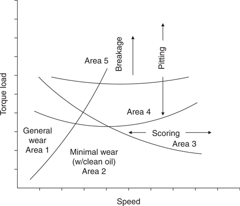
FIGURE 28.7
Regions of gear failures. (From Townsend, D.P., Dudley’s Gear Handbook: The Design Manufacture and Application of Gears, McGraw Hill, New York, NY, 1992.)
28.5.1.1.2 Gearbox Failure Conditions
Referring to Figure 28.7, in Area 1, the gear is operating too slowly to develop an oil film, so adhesive wear occurs. In Area 2, the speed is sufficiently fast to develop an oil film. The gears should be able to run with minimal wear. In Area 3, scoring is likely because the load and speed are high enough to break down the existing oil film. Area 4 illustrates the dominance of pitting caused by high surface stresses that result from higher torque loads. As the torque is increased further, tooth breakage will result from overload and stress fatigue, as shown in Area 5.
On the basis of earlier discussion, the MDTB test plan includes test runs that set the operating drive speed and load torque deep into each area to generate transitional data for each of the faults. These limits, of course, are not known exactly a priori. Areas 4 and 5 are the primary focal points because they contain critical and difficult-to-predict faults. Being able to control (to a degree) the conditions that affect the type of failure that occurs allows some control over the amount of data for each fault, while still allowing the fault to develop naturally (i.e., the fault is not seeded). If a particular type of fault requires more transitional data for analysis, adjustment of the operating conditions can increase the likelihood of producing the desired fault.
28.5.1.1.3 Oil Debris Analysis
Roylance and Raadnui36 examined the morphology of wear particles in circulating oil and correlated their occurrences with wear characteristics and failure modes of gears and other components of rotating machinery. Wear particles build up over time even under normal operating conditions. However, the particles generated by benign wear differ markedly from those generated by the active wear associated with pitting, abrasion, scuffing, fracturing, and other abnormal conditions that lead to failure. Roylance and Raadnui36 correlated particle features (quantity, size, composition, and morphology) with wear characteristics (severity, rate, type, and source).
Particle composition can be an important clue to the source of abnormal wear particles when components are made of different materials. The relationship of particle type to size and morphology has been well characterized by Roylance,36 and is summarized in Table 28.1.
28.5.1.1.4 Vibration Analysis
Vibration analysis is extremely useful for gearbox analysis and gear failures because the unsteady component of relative angular motion of the meshing gears provides the major source of vibratory excitation.37 This effect is largely caused by a change in compliance of the gear teeth and deviation from perfect shape. Such a modulated gear-meshing vibration, y(t), is given by
TABLE 28.1
Wear Particle Morphology—Ferrography Descriptors

where an(t) and bn(t) are the amplitude and phase modulation functions, respectively. Amplitude modulation produces sidebands around the carrier (gear-meshing and harmonics) frequencies and is often associated with eccentricity, uneven wear, or profile errors. As can be seen from the Equation 28.9, frequency modulation will produce a family of sidebands. These will typically occur in gear systems, and the sidebands, which may either combine or subtract to produce an asymmetrical family of sidebands.
Much of the analysis has focused on the use of the appropriate statistical processing and transforms to capture these effects. A number of figures of merit or features have been used to correlate mechanical faults. Moreover, short-time Fourier, Hilbert, and wavelet transforms have also been used to develop vibration features.38,39
28.5.1.1.5 Description of Features
Various signal and spectral modeling techniques have been used to characterize machinery data and develop features indicative of various faults in the machinery. Such techniques include statistical modeling (e.g., mean, RMS, kurtosis), spectral modeling (e.g., Fourier transform, cepstral transform, autoregressive modeling), and time frequency modeling (e.g., short-time Fourier transform, wavelet transform, wide-band ambiguity functions). Several oil and vibration features are now well described. These can be fused and integrated with knowledge of the system and history to provide indication of gearbox condition. In addition to the obvious corroboration and increased confidence that can be gained, this approach to using multiple sensors also aids in establishing the existence of sensor faults.
Features tend to organize into subspaces in feature space, as shown in Figure 28.8. Such subspaces can be used to classify the failure mode. Multiple estimates of a specific failure mode can be produced through the classification of each feature subspace. Other failure mode estimates can be processed at the same time as well. Note that a gearbox may deteriorate into more than one failure mode with several critical faults competing.

FIGURE 28.8
Oil/vibration data fusion process. (From Byington, C.S. et al., Proceedings of the 53rd Meeting of the Society for MFPT, 1999.)
During 20+ run-to-failure transitional tests conducted on the MDTB, data were collected from accelerometer, temperature, torque, speed, and oil quality/debris measurements. This discussion pertains only to Test 14. Borescope imaging was performed at periodic intervals to provide damage estimates as ground truth for the collected data. Small oil samples of a ∙25 mL were taken from the gearbox during the inspection periods. Postrun oil samples were also sent to the DoD Joint Oil Analysis Program (JOAP) to determine particle composition, oil viscosity, and particle-wear type.
The break-in and design load time for Test 14 ran for 96 h. The 3.33 ratio gearbox was then loaded at three times the design load to accelerate its failure, which occurred ∙20 h later (including inspection times). This load transition time was at ∙1200 (noon), and no visible signs of deterioration were noted. The run was stopped every 2 h for internal inspection and oil sampling. At 0200 (2:00 a.m.), the inspection indicated no visible signs of wear or cracks. After 0300, accelerometer data and a noticeable change in the sound of the gearbox were noted. On inspection, one of the teeth on the follower gear had separated from the gear. The tooth had failed at the root on the input side of the gear with the crack rising to the top of the gear on the load side (refer to Figure 28.9). The gearbox was stopped again at 0330, and an inspection showed no observable increase in damage. At 0500, the tooth from the downstream broken tooth had suffered surface pitting, and there were small cracks a millimeter in from the front and rear face of the tooth, parallel to the faces. The 0700 inspection showed that two teeth had broken and the pitting had increased, but not excessively, even at three times design load. Neighboring teeth now had small pits at the top-motor side corners.

FIGURE 28.9
Number of particles/milliliter for fatigue, cutting, and sliding wear modes (>15 µm) collected at various times.
On shutdown at 0815, with a significant increase in vibration (over 150% RMS), the test was concluded, eight teeth had suffered damage. The damaged teeth were dispersed in clusters around the gear. There appeared to be independent clusters of failure processes. Within each cluster a tooth that had failed as a result of root cracking was surrounded by teeth that had failed due to pitting. On both clusters, the upstream tooth had failed by cracking at the root, and the follower tooth had experienced pitting.
Figure 28.9 shows the time sequence of three types of particle concentrations observed during this test run: fatigue wear, cutting wear, and severe sliding wear. Initial increases in particle counts observed at 1200 reflect debris accumulations during break-in. Fatigue particles manifested the most dramatic change in concentration of the three detectable wear particle types, nearly doubling between 1400 and 1800, suggesting the onset of some fault that would give rise to this type of debris. This data is consistent with the inspections that indicated pitting was occurring throughout this time period. No significant sliding or cutting wear was found after break-in.
Figure 28.10 illustrates the breakdown of these fatigue particle concentrations by three different micrometer size ranges. Between 1400 and 1800, particle concentrations increased for all three ranges with onset occurring later for each larger size category. The smallest size range rose to over 1400 particles/mL by 1800, whereas the particles in the midrange began to increase consistently after 1400 until the end of the run. The largest particle size shows a gradual upward trend starting at 1600, though the concentration variation is affected by sampling/measurement error. The observed trends could be explained by hypothesizing the onset of a surface fatigue fault condition sometime before 1600, followed by steadily generated fatigue wear debris.
Figures 28.11 and 28.12 show different features of the accelerometer data developed at Penn State ARL. The results with a Penn State ARL enveloping technique (Figure 28.11) clearly show evidence of some activity around 0200. The dashed line represents the approximate time the feature showed a notable change. This corresponds to the time when tooth cracking is believed to have initiated/propagated. The wavelet transform40 is shown in Figure 28.12. It is believed to be sensitive to the impact events during breakage, and shows evidence of this type of failure after 0300. The processed indicators seem to indicate activity well before RMS levels provided any indication.

FIGURE 28.10
Number of fatigue-wear particles/milliliter by bin size collected at various times.

FIGURE 28.11
Interstitial enveloping of accelerometer.
During each stop, the internal components appeared normal until after 0300, when the borescope verified a broken gear tooth. This information clearly supports the RMS and wavelet changes. The changes in the interstitial enveloping that occurred around 0200 (almost 1 h earlier) could be considered as an early indicator of the witnessed tooth crack. Note that the indication is sensitive to threshold setting, and the MDTB online wavelet detection threshold triggered about an hour (around the same time as the interstitial) before that shown in Figure 28.12.
28.5.1.1.6 Feature Fusion
Although the primary failure modes on MDTB gearboxes have been gear tooth and shaft breakage, pitting has also been witnessed.41 On the basis of previous vibration and oil debris figures in this section, a good overlap of candidate features appears for both commensurate and noncommensurate data fusion. The data from the vibration features in Figure 28.13 show potential clustering as the gearbox progresses toward failure. Note from the borescope images that the damage progresses in clusters, which increase on both scales. The features in this subspace were obtained from the same type of sensor (i.e., they are commensurate). Often two noncommensurate features—such as oil debris and vibration—are more desirable.
Figure 28.14 shows a subspace example using a vibration feature and an oil debris (fatigue particle count) feature. There are fewer data points than in the previous example because the MDTB had to be shut down to extract an oil sample as opposed to using on-demand, DAQ collection of accelerometer data. During the progression of the run, the features seemed to cluster into regions that are discernible and trackable. Subspaces using multiple features from both commensurate and noncommensurate sources would provide better information for classification, as would the inclusion of running conditions, system knowledge, and history. This type of association of data is a necessary step toward accomplishing more robust state estimation and higher levels of data fusion.

FIGURE 28.12
Continuous wavelet transform (IIR count).

FIGURE 28.13
Feature subspace classification example.

FIGURE 28.14
Noncommensurate feature subspace.
28.5.1.1.7 Decision Fusion Analysis
Decision fusion is often performed as a part of reasoning in CBM systems. Automated reasoning and data fusion are important for CBM. Because the monitored systems exhibit complex behavior, there is generally no simple relationship between observable conditions and system health. Furthermore, sensor data can be very unreliable, producing a high false alarm rate. Hence, data fusion and automated reasoning must be used to contextually interpret the sensor data and model predictions. In this section, three automated reasoning techniques, neural networks (NNs), FL, and expert/rule-based systems, are compared and evaluated for their ability to predict system failure.42 In addition, these system outputs are compared to the output of a hybrid system that combines all three systems to realize the advantages of each. Such a quantitative comparison is essential in producing high-quality, reliable solutions for CBM problems; however, it is rarely performed in practice.
Although expert systems (ESs), FL systems, and NNs are used in machinery diagnostics, they are rarely used simultaneously or in combination. A comparison of these techniques and decision fusion of their outputs was performed using the MDTB data. In particular, three systems were developed (ES, FL, and NN) to estimate the RUL of the gearbox during accelerated failure runs (Figure 28.15). The inputs to the systems consisted of speed, torque, temperature, and vibration RMS in several frequency bands.

FIGURE 28.15
Flow diagram for comparison of three reasoning methods with mechanical diagnostic test bed data.
A graphical tool was developed to provide a quick visual comparison of the outputs of the different types of systems (Figure 28.16). In this tool, colors are used to represent the relative levels of the inputs and outputs and a confidence value is provided with each output. The time-to-failure curves for the three systems and the hybrid system are shown in Figure 28.17. In this example, the FL system provided the earliest warning, but the hybrid system gave the best combination of early warning and robustness.
28.5.2 Fluid Systems
Fluid systems comprise lubrication,20 fuel,43 and hydraulic power application examples. Some efforts at evaluating a model-based, data fusion approach for fluid systems are discussed in the following sections. Such fluid systems are critical to many navy engine and power systems and, clearly, must be a part of the CBM solution.
28.5.2.1 Lubrication System Function
A pressure-fed lubrication system is designed to deliver a specific amount of lubricant to critical, oil-wetted components in engines, transmissions, and like equipment. The primary function of a lubricant is to reduce friction through the formation of film coatings on loaded surfaces. It also transports heat from the load site and prevents corrosion. The lubricating oil in mechanical systems, however, can be contaminated by wear particles, internal and external debris, foreign fluids, and even internal component (additive) breakdown. All of these contaminants affect the ability of the fluid to accomplish its mission of producing a lubricious (hydrodynamic, elastohydrodynamic, boundary, or mixed) layer between mechanical parts with relative motion.44,45

FIGURE 28.16
Graphical viewer for comparing the outputs of the reasoning systems.

FIGURE 28.17
Time-to-failure curves for the reasoning systems with mechanical diagnostic test bed data.
TABLE 28.2
Lubricant and Wetted Component Faults

Lubricant contamination can be caused by many mechanisms. Water ingestion through seals (common in marine environments) or condensation will cause significant viscosity effects and corrosion. Fuel leakage through the (turbine fuel–lube oil) heat exchanger will also adversely affect lubricity. Moreover, fuel soot, dirt, and dust can increase viscosity and decrease the oil penetration into the loaded surface of the gears or bearings.46 An often overlooked, but sometimes significant, source of contamination is the addition of incorrect or old oil to the system. Table 28.2 provides a list of relevant faults that can occur in oil lubrication systems and some wetted components’ faults.
Many off-line, spectroscopic and ferrographic techniques exist to analyze lubricant condition and wear-metal debris.47, 48, 49, 50 and 51 These methods, although time-proven for their effectiveness at detecting many types of evolving failures, are performed at specified time intervals through off-line sampling.52 The sampling interval is driven by the cost to perform the preventive maintenance versus the perceived degradation window over an operational timescale. The use of intermittent condition assessment will miss some lubricant failures. Moreover, the use of such off-line methods is inconvenient and increases the preventive maintenance cost and workload associated with operating the platform.
28.5.2.2 Lubrication System Test Bench
A lubrication system test bench (LSTB) was designed to emulate the lubrication system of a typical gas turbine engine.53,54 The flow rate relates to typical turbine speeds, and flow resistance can be changed in each of the three legs to simulate bearing heating and differences between various turbine systems. To simplify operation, the LSTB uses facility water rather than jet fuel in the oil heat exchanger. The LSTB is also capable of adding a measured amount of foreign matter through a fixed-volume, dispensing pump, which is used to inject known amounts of metallic and nonmetallic debris, dirty oil, fuel, and water into the system. Contaminants are injected into a mixing block and pass through the debris sensors, upstream of the filter. The LSTB provides a way to correlate known amounts of contaminants with the system parameters and, thus, establishes a relationship between machinery wear levels, percentage of filter clogged, and viscosity of the lubricant.
The failure effects are in the areas of lubricant degradation, contamination, debris generated internally or externally, flow blockage, and leakage. These effects can be simulated or directly produced on the LSTB. Both degradation and contamination will result in changes in the oil transport properties. Water, incorrect oil, and sludge can be introduced in known amounts. Debris can be focused on metallic particles of 100 µm mean diameter, as would be produced by bearing or gear wear. Flow blockage can be emulated by restricting the flow through the control valves. Similarly, leakage effects can be produced by actual leaks or by opening the leg valves. Alternatively, seal leakage effects can cause air to flow into the lube system. This dramatically affects the performance and is measurable. In addition, the LSTB can be used to seed mechanical faults in the pump, relief valve, and instrumentation. In the case of mechanical component failure, vibration sensors could be added.
28.5.2.3 Turbine Engine Lubrication System Simulation Model and Metasensors
Note that the association of failure modes to sensor and fused data signatures remains a hurdle in such CBM work. Evaluation of operational data gathered on the gas turbine engine provided some association to believed faults, but insufficient data on key parameters prevented the implementation of a fault tree or even an implicit association. Given the lack of failure test data and the limited data available on the actual engine, a simulation model was developed. The turbine engine lubrication system simulation (TELSS) output was used to generate virtual or metasensor outputs. This data was evaluated in the data fusion and automated reasoning modules.
The TELSS consists of a procedural program and a display interface. The procedural program is written in C code and uses the analog of electrical impedances to model the oil flow circuit. The model contains analytical expressions of mass, momentum, and energy equations, as well as empirical relationships. The interface displays state parameters using an object-oriented development environment. Both scripted and real system data can be run through the simulation. A great deal of effort was expended to properly characterize the Reynolds number and temperature-dependent properties and characteristics in the model. TELSS requires the geometry of the network, the gas generator speed, and a bulk oil temperature to estimate the pressures and flows throughout.55
28.5.2.4 Data Fusion Construct
The initial approach for lubrication system data fusion is summarized in Figure 28.18. This example follows the previous methodology of reviewing the data fusion steps within the context of the application. There are five levels in the data fusion process:
Observation. This level involves the collection of measured signals from the lubrication system being monitored (e.g., pressures, flow rates, pump speed, temperatures, debris sensors, and oil quality measurements).
Feature extraction. At this level, modeling and signal processing begins to play a role. From the models and signal processing, features (e.g., virtual sensor signals) are extracted; features are more informative than the raw sensor data. The modeling provides additional physical and historical information.
Data association. In this level, the extracted features are mapped into commensurate and noncommensurate failure mode spaces. In other words, the feature data is associated with other feature data based on how they reveal the development of different faults.
System state estimation. In this level, classification of feature subspaces is performed to estimate specific failure modes of the lubricant or oil-wetted components in the form of a state estimate vector. The vector represents a confidence level that the system is in a particular failure mode; the classification also includes information about the system and history of the lubrication system.
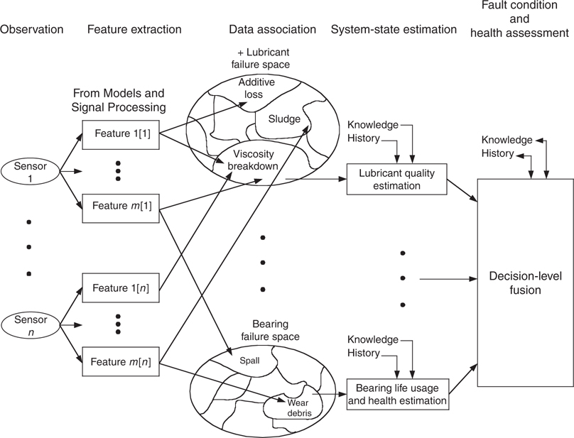
FIGURE 28.18
Lubrication system diagnostics/prognostics data fusion structure.Fault condition and health assessment. For this level, system health decisions are made based on the agreement, disagreement, or lack of information that the failure mode estimates indicate. The decision processing should consider which estimates come from commensurate feature spaces and which features map to other failure mode feature subspaces, as well as the historical trend of the failure mode state estimate.
28.5.2.5 Data Analysis Results
28.5.2.5.1 Engine Test Cell Correlation
Engine test cell data was collected to verify the performance of the system. The lubrication system measurements were processed using the data fusion toolkit to produce continuous data through interpolation. Typical data is seen in Figure 28.19. This data provided the opportunity to trend variables against the fuel flow rate to the engine, gas generator speed and torque, and the power turbine speed and torque. Ultimately, through various correlation analysis methods, the gas generator was deemed the most suitable regression (independent) variable for the other parameters. It was used to develop three-dimensional maps and regressions with a measured temperature to provide guidelines for normal operation.

FIGURE 28.19
Processing of test stand data and correlation in the ARL data fusion toolkit.
28.5.2.5.2 Operational Data with Metasensor Processing
Operational data was made available by a navy unit that uses the gas turbine engines. The operational data was limited to the production engine variables, which consisted of one pressure and temperature. The TELSS model was embedded within the multisensor fusion toolkit. The TELSS interface for an LPAS run is shown in Figure 28.20. Because the condition of the oil and filter was unknown for these runs, the type of oil and a specified amount of clogging was assumed. The variation of oil and types of filters can vary the results significantly. Different MIL-L-23699E oils, for many of which the model possesses regressions, can vary the flow rate predictions by up to 5%. Similar variation is seen when trying to apply the filter clogging to different vendors’ filter products.
The TELSS simulation model can be used to simulate different fault conditions to allow data association and system state estimation. Figure 28.21 illustrates the output of the metasensor under simulated fault conditions of filter clogging with debris. Filter clogging is typically monitored through a differential pressure measurement or switch. This method does not account for other variables that affect the differential pressure. The other variables are the viscosity, or the fluid resistance to flow, which is dependent on temperature and the flow rate through the filter.
With this additional knowledge, the T-P–mdot relationship can be exploited in a predictive fashion. Toward the mid to latter portion of the curves, the pressure increases slightly, but steadily, as the flow rate remains constant or decreases. Meanwhile, the temperature increases around 1000 s and then decreases steadily from 1500 until the engine is shut off. Let us investigate these effects more closely. The increasing pressure drop from about 1200 to 1500 s occurs whereas the temperature and flow are approximately constant. This is one indication of a clogging effect. From 1500 through 2100, the flow rate is at a lower level, but the pressure drop rises above its previous level at the higher oil flow rate. Looking only at these two variables could suffice; however, deeper analysis reveals that during the same timeframe, the temperature decreases, which means the viscosity (or resistance to flow) of the oil increases. This lower temperature would indicate that higher pressure drops could be expected for the same flow rate. This effect (increased viscosity due to lower temperature) is the reason why the pressure drop is so high at the beginning of the run. Consequently, this consideration actually adds some ambiguity to an otherwise crisp indication. The model analysis indicates, though, that the additional pressure drop caused by higher viscosity does not comprise the entire difference. Thus, the diagnosis of filter clogging is confirmed in light of all of the knowledge about the effects.

FIGURE 28.20
TELSS processing of operational data to produce metasensors. Massflow in pounds per hour is shown in bar scaled objects. Pressure throughout the circuit in pounds per square inch is illustrated by pressure gauge objects.
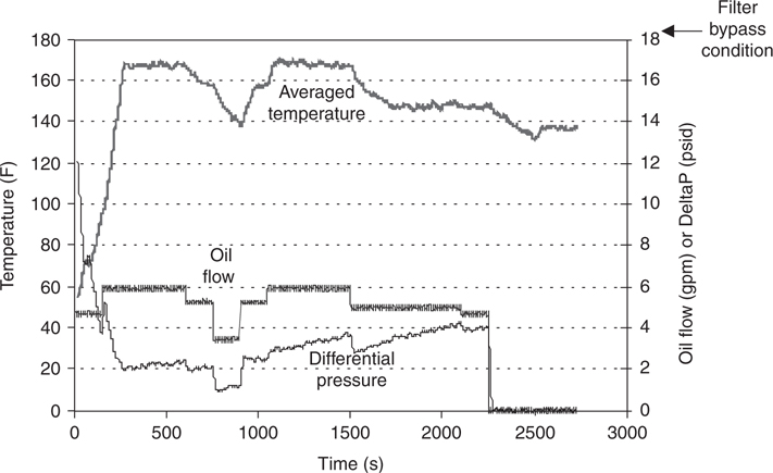
FIGURE 28.21
TELSS run illustrating the relationship between the system variables that can be fused to produce filter clogging association and estimates.
28.5.2.6 Health Assessment Example
The output from the TELSS model and multisensor toolkit was processed using an automated reasoning shell tool (Figure 28.22). The output of a shell that could be used to detect filter-clogging fractions is shown in the figures below. An ES, a FL association, and a NN perform the evaluations of filter clogging. The flow, temperature, and differential pressure were divided into three operational ranges. The ES was provided set values for the fraction clogged. The FL was modeled with trapezoidal membership functions. The NN was trained using the FL outputs.55,56 For the first case shown, the combination of 4.6 gpm, 175°F, and 12 psid, the reasoning techniques all predict relatively low clogging. In the next case, the flow is slightly less, whereas the pressure is slightly higher at 12.5 psid. The NN evaluation quickly leans toward a clogged filter, but the other techniques lag in fraction clogged. The ES is not sensitive enough to the relationships between the variables and the significance of the pressure differential increasing while the flow decreases markedly. This study and others conducted at ARL indicated that a hybrid approach based on decision fusion methods would allow the greatest flexibility in such assessments.

FIGURE 28.22
Hybrid reasoning shell evaluation (cases a and b).
28.5.2.7 Summary
The objective of this fluid systems research was to demonstrate an improved method of diagnosing anomalies and maintaining oil lubrication systems for gas turbine engines. Virtual metasensors from the TELSS program and operational engine data sets were used in a hybrid reasoning shell. A simple module for the current-limited sensor suite on the test engine was proposed, and recommendations for enhanced sensor suites and modules were provided. The results and tools, although developed for the test engine, are applicable to all gas turbine engines and mechanical transmissions with similar pressure-fed lubrication systems.
As mentioned in Section 28.5.2.5.2, the ability to associate faulted conditions with measurable parameters is tantamount for developing predictive diagnostics. In the current example, metasensors were generated using model knowledge and measured inputs that could be associated to estimate condition. Development of diagnostic models results from the fusion of the system measurements as they are correlated to an assessed damage state.
28.5.3 Electrochemical Systems
Batteries are an integral part of many operational environments and are critical backup systems for many power and computer networks. Failure of the battery can lead to loss of operation, reduced capability, and downtime. A method to accurately assess the condition (state-of-charge, SOC), capacity (amp-h), and remaining charge cycles (RUL) of primary and secondary batteries could provide significant benefit. Accurate modeling characterization requires electrochemical and thermal elements. Data from virtual (parametric system information) and available sensors can be combined using data fusion. In particular, information from the data fusion feature vectors can be processed to achieve inferences about the state of the system.
This section describes the process of computing battery SOC—a process that involves model identification, feature extraction, and data fusion of the measured and virtual sensor data. In addition to modeling the primary electrochemical and thermal processes, it incorporates the identification of competing failure mechanisms. These mechanisms dictate the RUL of the battery, and their proper identification is a critical step for predictive diagnostics.
Figure 28.23 illustrates the model-based prognostics and control approach that the battery predictive diagnostics project addresses. The modeling approach to prognostics requires the development of electrical, chemical, and thermal model modules that are linked with coupled parameters. The output of the models is then combined in a data fusion architecture that derives observational synergy, while reducing the false alarm rate. The reasoning system provides the outputs shown at the bottom right of the figure. Developments will be applicable to the eventual migration of the diagnosis and health monitoring to an electronic chip embedded into the battery (i.e., intelligent battery health monitor).
28.5.3.1 The Battery as a System
A battery is an arrangement of electrochemical cells configured to produce a certain terminal voltage and discharge capacity. Each cell in the battery is comprised of two electrodes where charge transfer reactions occur. The anode is the electrode at which an oxidation (O) reaction occurs. The cathode is the electrode at which a reduction (R) reaction occurs. The electrolyte provides a supply of chemical species required to complete the charge transfer reactions and a medium through which the species (ions) can move between the electrodes. Figure 28.24 illustrates the pathway ion transfer that takes place during the reaction of the cell.57,58 A separator is generally placed between the electrodes to maintain proper electrode separation despite deposition of corrosion products.57 Electrochemical reactions that occur at the electrodes can generally be reversed by applying a higher potential that reverses the current through the cell. In situations where the reverse reaction occurs at a lower potential than any collateral reaction, a rechargeable or secondary cell can potentially be produced. A cell that cannot be recharged because of an undesired reaction or an undesirable physical effect of cycling on the electrodes is called a primary cell.57

FIGURE 28.23
Model-based prognostics and control approach.

FIGURE 28.24
Electrode reaction process. (From Berndt, D., Maintenance-Free Batteries, Wiley, New York, NY, 1997; Bard, A.J. and Faulkner, L.R., Electrochemical Methods: Fundamentals and Applications, Wiley, New York, NY, 1980.)
Changes in the electrode surface, diffusion layer, and solution are not directly observable without disassembling the battery cell. Other variables such as potential, current, and temperature are observable and can be used to indirectly determine the performance of physical processes. For overall performance, the capacity and voltage of a cell are the primary specifications required for an application. The capacity is defined as the time integral of current delivered to a specified load before the terminal voltage drops below a predetermined cut-off voltage. The present condition of a cell is described nominally with the SOC, which is defined as the ratio of the remaining capacity and the total capacity. Secondary cells are observed to have a capacity that deteriorates over the service life of the cell. The term state-of-health (SOH) is used to describe the physical condition of the battery, which can range from external behavior, such as loss of rate capacity, to internal behavior, such as severe corrosion. The remaining life of the battery (i.e., how many cycles remain or the usable charge) is termed the state-of-life (SOL).
28.5.3.2 Mathematical Model
An impedance model called the Randles circuit, shown in Figure 28.25, is useful in assessing battery condition. Impedance data can be collected online during discharge and charge to capture the full change of battery impedance and identify the model parameters at various stages of SOC, as well as over multiple cycles of the battery for SOH identification. Some of the identified model parameters of the nickel–cadmium battery are shown in Figure 28.26 as the batteries proceed from a fully charged to a discharged state. Identification of these model-based parameters provides insight and observation into the physical processes occurring in the electrochemical cell.59,60

FIGURE 28.25
Two-electrode randles circuit model with wiring inductance.

FIGURE 28.26
Nickel–cadmium model parameters over discharge cycle.
28.5.3.3 Data Fusion of Sensor and Virtual Sensor Data
The approach for battery feature data fusion is summarized in Figure 28.27. There are five levels in the data fusion processes: observation (data collection), feature extraction (computation of model parameters and virtual sensor features), data association (mapping features into commensurate and noncommensurate feature spaces), system-state estimation (estimation of failure modes and confidence level), and fault condition and health assessment (making system health decisions).
Figure 28.28 illustrates the sensor and virtual sensor input to the data fusion processing. The outputs of the processing are the SOC, SOH, and SOL estimates that are fed into the automated reasoning processing. After the data association processing, an estimate of the failure mechanism is determined.
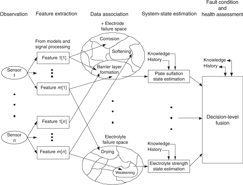
FIGURE 28.27
Battery diagnostics/prognostics data fusion structure.

FIGURE 28.28
Generalized feature vector for battery predictive diagnostics.
Two approaches for SOC prediction are described in Sections 28.5.3.3.1 and 28.5.3.3.2. Each performs a kind of data fusion to utilize physically meaningful parameters to predict SOC. The definition of SOC is the amount of useful capacity remaining in a battery during a discharge. Thus, 100% SOC indicates full capacity and 0% SOC indicates that no useful capacity remains.
28.5.3.3.1 ARMA Prediction of State-of-Charge
An effective way to predict SOC of a battery has been developed using ARMA model methodology.61 This model has performed well on batteries of various size and chemistry, as well as at different temperatures and loading conditions. ARMA models are a very common system identification technique because they are linear and easy to implement. The model used in this application is represented by
where y represents SOC; X represents a matrix of model inputs; and a, b, and c0 represent the ARMA coefficients. Careful consideration was exercised in determining the inputs. These were determined to be VD, ID, RΩ, θ, CDL, and Ts, and output is SOC. The inputs were smoothed and normalized to reduce the dependence on noise and to prevent domination of the model by parameters with the largest magnitudes.
The model was determined by using one of the runs and then tested with the remaining runs. Figure 28.29 shows the results for all eight size-C batteries. The average prediction error for lithium batteries was <3%, for NiCad <5%, and for lead acid <10%. These results are summarized in Table 28.3.

FIGURE 28.29
ARMA SOC prediction results for size-C lithium (CF)x batteries.
TABLE 28.3
Results of ARMA Model SOC Predictions

28.5.3.3.2 Neural Networks Prediction of State-of-Charge
Artificial NNs have been used successfully in both classification and function approximation tasks.61 One type of function approximation task is system identification. Although NNs very effectively model linear systems, their main strength is the ability to model nonlinear systems using examples of input–output pairs. This was the basis for choosing NNs for SOC estimation. NN SOC estimators were trained for lithium batteries of sizes C and 2/3 A under different loading conditions. For each type of battery, a subset (typically 3–6) of the available parameter vectors was chosen as the model input. Networks were trained to produce either a direct prediction of battery SOC or, alternatively, an estimation of initial battery capacity during the first few minutes of the run.
All networks used for battery SOC estimation had one hidden layer. The back propagation, gradient-descent learning algorithm is used, which utilizes the error signal to optimize the weights and biases of both network layers. The inputs to the network were a subset of ID, VD, RΩ, θ, and CDL. As for the ARMA case, the inputs were smoothed and normalized. This led to smaller networks, which tend to be better at generalization. For time-delay NNs, the selection of the number of delays and the length of the delays is crucial to the performance of the networks. Both short and long delays were tried during different training runs. The short delays gave better performance, which indicates that the battery SOC does not involve long time constants. This is also evident from the ARMA examples. Several types of NNs were trained with battery data and extracted impedance parameters to directly predict the battery SOC. Among the several training methods that were used, the Levenberg–Marquardt (L-M) provided the best results. The size of the network was also important in training. An excessively small network size results in inadequate training, and a larger than necessary network size leads to over-training and poorer generalization.
NNs trained to directly provide the battery SOC provided consistently good performance. However, the performance was much better when the battery’s initial capacity was first estimated. These networks were also trained to estimate the initial capacity of the battery during the first few minutes of the test. Then, the measured load current could easily be used to predict SOC because the current is the rate of change of charge. This is even more useful for SOH and SOL prediction because as the secondary batteries are reused they start at different initial capacity each time.
This method can also be used as a powerful tool in mission planning. Hypothetical load profiles can be used to predict whether a battery would survive or fail a given mission, thus preventing the high cost and risk of batteries failing in the field. The networks tend to slightly underestimate the battery SOC. This is a very important practical feature, since it results in a conservative estimate and avoids unscheduled downtime.
The results using radial basis function (RBF) NNs were the best and are summarized in Table 28.4. The SOC plots are shown for size-C lithium batteries in Figure 28.30. The results are quite remarkable, considering that very little training data are required to produce the predictors. As more data are collected and several runs of each of level of initial battery SOC become available, the robustness of the predictors will likely improve. In addition, the NN predictors have smaller error on outliers and provide a conservative prediction (i.e., they do not over-predict the SOC). Both of these advantages are very important in practical systems where certification and low false alarms are not just requirements, but can make the difference between a system that is actually used or shelved.
TABLE 28.4
Error Rates for SOC Prediction Based on Initial Capacity Estimation with RBF Neural Networks
Battery Size (Number of Hidden Neurons) |
Average Training Error (Training Set) |
Average Testing Error |
Maximum Testing Error (Run Number) |
Size C6 |
2.9% |
6.8%15 |
|
Size 2/3 A12 |
2.9% |
8.2%23 |

FIGURE 28.30
SOC prediction for size-C lithium batteries using initial SOC estimation with RBF neural networks.
28.6 Concluding Remarks
The application of data fusion in the field of CBM and predictive diagnostics for engineered systems is rich with opportunity. The authors fully acknowledge that only a small amount of what is possible to accomplish with data fusion has been presented in this chapter. The predictive diagnostics application domain is relatively new for data fusion, but the future is bright with the many analogies that can be drawn between more mature data fusion applications and the current one. The authors anticipate that continuing developments in actual and virtual feature fusion, as well as hybrid decision fusion of condition assessments, will tend to dominate the research field for some time.
Acknowledgments
The authors gratefully acknowledge support from Dr. Thomas McKenna and Dr. Phillip Abraham from the Office of Naval Research on grant numbers N00014-95-1-0461, N00014-96-1-0271, N00014-97-1-1008, and N00014-98-1-0795, under which most of this work was originally performed. The authors would also like to acknowledge the contributions of several past and present colleagues at the Applied Research Laboratory: Mr. Bill Nickerson for his vision, help in understanding a framework for the CBM problem, and contributions to the definitions and systems thinking sections; Mr. James Kozlowski for his work on gearbox and battery diagnostics data fusion; Mr. Derek Lang for his work on the multisensor toolkit and insight into decision fusion; Mr. Dan McGonigal for his help in programming the lubrication system example and automated reasoning work on the gearbox failure tests; Mr. Jerry Kasmala for his development and assistance in the use of the data fusion toolkit; Ms. Terri Merdes for her contributions to the oil-vibration fusion analysis and discussion; Mr. Thomas Cawley for his development of a battery mathematical model; Mr. Matthew Watson for his work on ARMA modeling for SOC prediction; Mr. Todd Hay for his contributions to the neural network prediction section; Ms. Natalie Nodianos for her insightful editing; and Dr. David Hall for his mentoring and pointing the compass for the CBM data fusion effort at Penn State ARL.
References
1. Hansen, R. J., Hall, D. L., and Kurtz, S. K., A new approach to machinery prognostics, Journal of Engineering for Gas Turbines and Power, 117(2), 320–325, DN: Presented at 39th International Gas Turbine and Aeroengine Congress and Exposition, June 13–16, 1994, The Hague (NL), PBD, April 1995.
2. Kotanchek, M. E. and Hall, D. L., CBM/IPD Process Model, ARL TM 95-113, November 1995.
3. Byington, C. and Nickerson, G. W., Technology issues for CBM, P/PM Technology Magazine, 9(3), June 1996.
4. Byington, C., Monitoring the health of mechanical transmissions, NCADT Quarterly, No. 2, 1996.
5. Chamberlain, M., U.S. Navy Pursues Air Vehicle Diagnostics Research, Vertiflite, Vol. 40, pp. 16–21, March/April 1994.
6. Douglas, J., The maintenance revolution, EPRI Journal, 207(9), 6–15, May/June 1995.
7. Condition-directed maintenance, Electric Power Research Institute, Compressed Air Magazine, August 1990.
8. Hall, D. L., Hansen, R. J., and Lang, D. C., The negative information problems in mechanical diagnostics, in Proceedings of the International Gas Turbine Institute Conference, ASME, Birmingham, England, June 1997.
9. Elverson, B., Machinery fault diagnosis and prognosis, M.S. Thesis, The Pennsylvania State University, 1997.
10. Erdley, J., Data fusion for improved machinery fault classification, M.S. Thesis, The Pennsylvania State University, May 1997.
11. Dempster, A. P., Generalization of Bayesian inference, Journal of Royal Statistical Society, 30(2), 205–247, 1968.
12. Shafer, G., A Mathematical Theory of Evidence, Princeton University Press, Princeton, NJ, 1976.
13. Thomopoulos, S. C. A., Theories in distributed decision fusion: Comparison and generalization, in Proceedings of the SPIE 1990 on Sensor Fusion III: 3-D Perception and Recognition, Boston, MA, pp. 623–634, November 5–9, 1991.
14. Hall, D. and McMullen, S. A. H., Mathematical Techniques in Multisensor Data Fusion, Artech House, Inc., Norwood, MA, 1992.
15. Waltz, E. and Llinas, J., Multisensor Data Fusion, Artech House, Inc., Boston, MA, 1990.
16. Bayes, T., An essay towards solving a problem in the doctrine of chances, Philosophical Transactions of the Royal Society of London, 53, 370–418, 1763.
17. Freund, J. E. and Walpole, R. E., Mathematical Statistics, 3rd. Ed., Prentice-Hall, Englewood Cliffs, NJ, 1980.
18. Pearl, J., Probabilistic Reasoning in Intelligent Systems, Morgan Kaufmann Series in Representation and Reasoning, San Francisco, CA, 1988.
19. Natke, H. G. and Cempel, C., Model-based diagnosis: Methods and experience, in Proceedings of a Joint Conference, the 51st Meeting of the Society for Machinery Failure Prevention Technology (MFPT) and the 12th Biennial Conference on Reliability, Stress Analysis and Failure Prevention (RSAFP Committee of ASME) (Henry C. Pusey and Sallie C. Pusey, Eds.), Virginia Beach, VA, pp. 705–719, April 14–18, 1997.
20. Byington, C. S., Model-Based Diagnostics for Turbine Engine Lubrication Systems, ARL TM98-016, February 1998.
21. Hall, D. L. and Kasmala, G., Visual programming environment (Toolkit) for multisensor data fusion, in Proceedings of the SPIE AeroSense 1996 Symposium, Orlando, FL, Vol. 2764, pp. 181–187, April 1996.
22. Hall, D. L. and Garga, A. K., Pitfalls in data fusion (and how to avoid them), in Proceedings of 2nd International Conference on Information Fusion (FUSION 99), Vol. I, pp. 429–436, 1999.
23. Begg, C., Merdes, T., Byington, C. S., and Maynard, K. P., Dynamics modeling for mechanical fault diagnostics and prognostics, in Maintenance and Reliability Conference, 1999.
24. Mitchell, L. D. and Daws, J. W., A Basic Approach to Gearbox Noise Prediction, SAE Paper 821065, Society of Automotive Engineers, Warrendale, PA, 1982.
25. Ozguven, H. N. and Houser, D. R., Dynamic analysis of high speed gears by using loaded static transmission error, Journal of Sound and Vibration, 125(1), 71–83, 1988.
26. Randall, R. B., A new method of modeling gear faults, Transactions of the ASME, Journal of Mechanical Design, 104, 259–267, 1982.
27. Nicks, J. E. and Krishnappa, G., Evaluation of vibration analysis for fault detection using a gear fatigue test rig, C404/022, in IMEC E Proceedings, 1990.
28. Zakrajsek, J. J., An investigation of gear mesh failure prediction techniques, NASA Technical Memorandum 102340 (89-C-005), November 1989.
29. Tandon, N. and Nakra, B. C., Vibration and acoustic monitoring techniques for the detection of defects in rolling element bearings: A review, The Shock and Vibration Digest, 24(3), 311, March 1992.
30. Li, C. J. and Wu, S. M., On-line detection of localized defects in bearings by pattern recognition analysis, Journal of Engineering for Industry, 111, 331–336, 1989.
31. Rose, J. H., Vibration Signature and Fatigue Crack Growth Analysis of a Gear Tooth Bending Fatigue Failure, Presented at 44th Meeting of the Mechanical Failure Prevention Group (MFPG), April 2–5, 1990.
32. Mathew, J. and Alfredson, R. J., The condition monitoring of rolling element bearings using vibration analysis, Journal of Vibration, Acoustics, Stress, and Reliability in Design, 106, 447–453, 1984.
33. Lebold, M., McClintic, K., Campbell, R., Byington, C., and Maynard, K., Review of vibration analysis methods for gearbox diagnostics and prognostics, in Proceedings of the 53rd Meeting of the Society for Machinery Failure Prevention Technology, Virginia Beach, VA, pp. 623–634, May 2000.
34. Byington, C. S. and Kozlowski, J. D., Transitional data for estimation of gearbox remaining useful life, in Proceedings of the 51st Meeting of the Society for Machinery Failure Prevention Technology (MFPT), Virginia Beach, VA, Vol. 51, pp. 649–657, April 1997.
35. Townsend, D. P., Dudley’s Gear Handbook: The Design Manufacture and Application of Gears, 2nd Ed., McGraw Hill, New York, NY, 1992.
36. Roylance, B. J. and Raadnui, S., The morphological attributes of wear particles: Their role in identifying wear mechanisms, Wear, 175, 115–121, 1995.
37. Brennan, M. J., Chen, M. H., and Reynolds, A. G., Use of vibration measurements to detect local tooth defects in gears, Sound and Vibration, November 1997.
38. Wang, W. J. and McFadden, P. D., Application of the wavelet transform to gearbox vibration analysis, in Structural Dynamics and Vibrations, American Society of Mechanical Engineers (ASME), in Proceedings of the 16th Annual Energy Sources Technology Conference and Exposition, Vol. 52, pp. 13–20, January 31–February 4, 1993.
39. Ferlez, R. J. and Lang, D. C., Gear tooth fault detection and tracking using the wavelet transform, in Proceedings of the 52nd Meeting of the MFPT, 1998.
40. Byington, C. S. et al., Vibration and oil debris feature fusion in gearbox failures, in Proceedings of the 53rd Meeting of the Society for MFPT, 1999.
41. Byington, C. S. et al., Fusion techniques for vibration and oil debris/quality in gearbox failure testing, International Conference of Condition Monitoring, Swansea, pp. 113–128, 1999.
42. McGonigal, D. L., Comparison of automated reasoning techniques for CBM, M.S. Thesis, The Pennsylvania State University, August 1997.
43. Campbell, R. L. and Byington, C. S., Gas turbine fuel system modeling and diagnostics, in COMADEM Proceedings, 13th International Congress on Condition Monitoring and Diagnostic Engineering Management, Houston, TX, pp. 257–266, December 2000.
44. Toms, L. A., Machinery Oil Analysis: Methods, Automation and Benefits, 2nd Ed., Coastal Skills training, Virginia Beach, VA, 1998.
45. Lubrication Fundamentals: Fundamental Concepts and Practices, Lubrication Engineering Magazine, 26–34, September 1997.
46. Eleftherakis, J. G. and Fogel, G., Contamination control through oil analysis, P/PM Technology Magazine, 62–65, October 1994.
47. Toms, A. M. and Powell, J. R., Molecular analysis of lubricants by FT-IR spectroscopy, P/PM Technology Magazine, 58–64, August 1997.
48. Richards, C., Oil analysis techniques advance with new information technology, P/PM Technology Magazine, 60–62, June 1995.
49. Neale, M. J., Component Failures, Maintenance, and Repair, Society of Automotive Engineers, Inc., Warrendale, PA, 1995.
50. Anderson, D. P., Rotrode filter spectroscopy: A method for the multi-elemental determination of the concentration of large particles in used lubricating oil, P/PM Technology Magazine, 88–89, September/October 1992.
51. Stecki, J. S. and Anderson, M. L. S., Machine condition monitoring using filtergram and ferrographic techniques, Research Bulletin: Machine Condition Monitoring, 3(1), September 1991.
52. Troyer, D. and Fitch, J. C., An introduction to fluid contamination analysis, P/PM Technology Magazine, 54–59, June 1995.
53. Byington, C. S., Model-based diagnostics of gas turbine engine lubrication systems, Joint Oil Analysis Program International Condition Monitoring Program, April 20–24, 1998.
54. Byington, C. S., Intelligent monitoring of gas turbine engine lubrication systems, ARL TN 98-016, February 1998.
55. Garga, A. K., A hybrid implicit/explicit automated reasoning approach for condition-based maintenance, in Proceedings of ASNE Intelligent Ships Symposium II, 1996.
56. Stover, J. A., Hall, D. L., and Gibson, R. E., A fuzzy-logic architecture for autonomous multisensor data fusion, IEEE Transactions of Industrial Electronics, 43(3), 403–410, June 1996.
57. Berndt, D., Maintenance-Free Batteries, 2nd Ed., Wiley, New York, NY, 1997.
58. Bard, A. J. and Faulkner, L. R., Electrochemical Methods: Fundamentals and Applications, Wiley, New York, NY, 1980.
59. Boukamp, A., A nonlinear least squares fit procedure for analysis of immittance data of electrochemical systems, Solid State Ionics, 20(31), 31–44, 1986.
60. Kozlowski, J. D. and Byington, C. S., Model-based predictive diagnostics for primary and secondary batteries, in Proceedings of the 54th Meeting of the MFPT, Virginia Beach, VA, May 1–4, 2000.
61. Kozlowski, J. D. et al., Model-based predictive diagnostics for electrochemical energy sources, in Proceedings of IEEE Aerospace Conference, Vol. 6, pp. 63149–63164, Big Sky, MT, March 2001.