31 Developing Information Fusion Methods for Combat Identification

The goal of Combat Identification (Combat ID or simply CID) fusion is to combine information at the appropriate information levels to derive a positive identification (ID) according to a classification structure. This in turn can help determine the allegiance of an object such as Friend, Neutral, or Hostile. Specifically, the overarching goal of CID is to attain an accurate characterization of detected objects in the joint battlespace so that high-confidence, timely application of military options and weapon resources can occur. A visualization of this concept is shown in Figure 31.1.¹

Figure 31.1 illustrates the essential problems with understanding, processing, and fusing information in this domain. No other fusion domain exists where not only are there multiple complexities such as friendly, hostile, and neutral relationships * to the identifying agent^† in addition to environmental confusor effects, but there may be objects that are actively attempting to deceive and evade detection and classification. This makes the design of a fusion process more difficult for CID than possibly for any other domain.

The decision of whether to engage or not engage an object may only occur very infrequently over a long period of time, especially if the identifying agent is not participating in an active or simulated battle-like situation. However, the results of poor CID are painfully well known. The USS Vincennes Airbus incident, the U.S. Army Black Hawk helicopter fratricide, and the Operation Iraqi Freedom (OIF) U.S. Army Patriot missile fratricides are some of the best-known examples. Many more occur in air-to-ground and ground-to-ground combat operations that are not as well documented, but make up the majority of the historical 7–25% rate of fratricides in major wars fought in the twentieth century.

Images

FIGURE 31.1
Warfighting domain complexities.

Referencing Kebodeaux,² one of the many goals on the battlefield throughout history has been to reduce friendly fire (fratricide) incidents. These misidentifications are, not surprisingly, a result of what Clausewitz termed the fog of war, which is another way of describing uncertainty. The problem is exacerbated by the raw speed of modern warfare, where the time between a weapon engagement decision and target impact is exceedingly short. Improving awareness is the same as improving information processing; thus, this reduces fogginess that provides improvement in decision quality. To adequately represent the warfighting domain as an abstraction that can be captured computationally and reproduced, a systems engineering approach to the design of a fusion/track management/CID/sensor management command and decision (C&D) system must be taken. Internal to this C&D system is the CID function that has historically not been considered properly from a systems and information engineering perspective. CID has traditionally been treated with disastrous oversimplification by emphasizing what was practical, rather than correct. Figure 31.2 illustrates the attribute information domain that must be exploited properly to achieve CID success.

Figure 31.2 illustrates the application of information engineering to generate an information model–based design which is a radical change for the concept of CID which has historically been rule based and developed from a cooperative-space information domain (due to the lack of sensors and information from other domain spaces). In this figure, it can be seen that kinematics and cooperative information form only a subset of the total information space that should be used to derive a CID. If disparate sets of sensors are used to provide high fidelity attribute data to a fusion process, then the more encompassing information domain space can be mastered and high-confidence positive Hostile, Suspect, and Neutral CID declarations (not just Friend) can be developed. This domain space consists of cooperative, noncooperative, and unintentionally cooperative information sets and spaces, which are expounded upon in this chapter.

Images

FIGURE 31.2
Attribute information space.

The purpose of performing CID fusion is to obtain correct and timely object identification. To achieve this, it is necessary to optimize the baseline of physical observations (attribute and kinematic measurements) to capture the entire object information domain space to the greatest extent possible, and then reconstruct a representation of the object. The human senses work in a similar fashion. The human brain fuses sight, hearing, smell, touch, and taste to form a representation of an object (such as spoiled fish—certainly unfriendly), which is then used as input to determine how the body should react. The behavior response to a car moving toward you with an engine that is roaring is very different than the same car without the same aural characteristic.

This approach also avoids the generation of CID conflicts that may arise when multiple platforms work from sparse information to derive identifications that will probabilistically differ due to violations of the principle of information entropy.* Further, by dominating the information sample space S in Figure 31.2 as completely as possible, it is possible to extract CID information even when sensor responses are conspicuously absent or contradictory, such as the case when an air object is in EMCON (Emission Control) or when spoofing is attempted. This is the concept of negative information and can be exploited when the state of the CID domain space is well known.

31.2 Mapping CID to JDL Levels

For the purpose of CID fusion, it is assumed the reader has some familiarity with the Joint Directors of Laboratories (JDL) model.^† However, a purposeful description is needed to clarify some concepts. Figure 31.3, originally described by White,³ presents a graphical description of the model.

The problem of parsing and fusing CID information falls within JDL levels 1, 2, and 3. Other levels not described at length are level 0 information that includes such operations as coherent signal processing of measurement data, centroiding and filtering of kinematic data, identification friend-or-foe (IFF) code degarbling, emitter classification, local association and tracking, and so on. This level of processing is generally performed entirely within individual sensors. Level 4 processing is a metaprocess that monitors and optimizes the overall data fusion performance via planning and control, not estimation as in JDL levels 1 through 3. The level 5 human–computer interaction at the right of Figure 31.3 is also sometimes referred to as level 5 fusion that is unique because it adds a human operator/decision maker in the loop. In the context of CID, the following discussion defines the type of information processed by the remaining JDL levels.

JDL level 1—object refinement. This processing level combines information from the results of level 0 processing within sensors. For CID, this is about fusing the attributes of objects so as to detect, locate, characterize, track, and classify these objects. This level of processing involves information assignment/correlation, and what is defined as taxonomic CID. This means assigning an identity to an object from a taxonomy—a set of mutually exclusive alternatives. Examples are the hierarchical taxonomies: category, platform, type, and class. Other examples are unit and nationality—although nationality is often considered to be a level 3 category.

Images

FIGURE 31.3
Joint Directors of Laboratories fusion model representation.

Examples of level 1 declarations include tank, M-1 Abrams, fighter, Destroyer, 737-300, and so on. The goal, therefore, of JDL level 1 processing is to determine exactly what an object is, not its relationship to the identifying node or platform. Taxonomic CID processing includes (1) information alignment such as time synchronization, and gridlock and bias removal, (2) information correlation (platform–platform, type–platform, class–type, etc.), and (3) probabilistic/evidential attribute estimation (Bayesian, Dempster–Shafer, etc.). Generally, to fuse information at this level, multiple hypotheses must be tracked. This is because taxonomic CID information from sources is available at different levels and often not sufficient to discriminate with certainty. Automating the fusion and declaration decision process flexibly across these levels, as information becomes available, without throwing away valuable information and context is challenging.

JDL level 2—situation refinement. This processing level includes the ability to establish contextual relationships of objects declared in level 1 processing with their environment. This includes situation refinement using some sort of assessment to declare an object as (1) Friend, (2) Assumed Friend, (3) Neutral, (4) Suspect, (5) Hostile, and (6) Unknown. This is also referred to as defining an object’s allegiance. Level 2 processing uses some sort of decision methodology such as if-then-else logic, voting fusion, or even Bayesian decision logic to derive the object state and establish the CID. For example, if an object is determined to have a high-confidence taxonomic CID of an F-16, this in itself offers no information on whether it is friendly toward the platform or node performing the identification. However, inserting a level 2 assessment decision will enable the proper CID declaration to occur based on such rules as country-of-origin, flight profile, intelligence information, and so on. In this example, doctrine (which historically defines some sort of rule set) could derive a CID of Assumed Friend if no hostile entities in the theater are known to have any F-16s in their inventories. Some sensor/source information may also be directly fused at this level, for example, secure cooperative information such as some IFF modes and data link self-identifications, if available. The presence of this type of secure information can be directly associated with the existence of a Friend, although the lack of it cannot normally imply a Hostile or Unknown designation. It is important to note that level 2 categories are drawn from a single taxonomy, so the structures for fusion are different from the ones best suited for the multiple taxonomies of level 1. This will be explained in the discussion of Figure 31.4 in Section 31.2.1.

Images

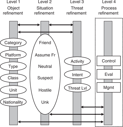
FIGURE 31.4
Multihypothesis structures with Joint Directors of Laboratories levels.

JDL level 3—threat refinement. This processing level attempts to interpret a situation from a dynamic behavior point-of-view and involves evaluating hypotheses concerning the future actions of an object and the potential consequences of those actions. This includes threat analysis and the assessment of intent if it is possible to get into the adversary’s decision cycle (as in the Boyd OODA loop *). For CID, this processing level can take the results of levels 1 and 2, in addition to independently processing information, and will determine if the identified object is a candidate for engagement. For example, using a self-defense scenario, if an object is positively identified as a Hostile, but is flying away from any defended assets and poses no threat, then the object’s intent may not be threatening and the identifying platform or node may choose not to engage it. Depending on the refinement in the level 1 processing, if platform type, class, unit, nationality, and activity are known, then this may be used along with the CID output at level 2 for level 3 processing. As an example, if an object is identified as Hostile, with a taxonomic identification of a military reconnaissance aircraft on a surveillance mission, then that object may not qualify for engagement because it has no offensive weapons capability (again depending on doctrine and situation). The methods of fusing and processing information at this level include Bayesian networks, neural networks, and Markov gaming.

31.2.1 Multihypothesis Structures

An information model for multihypothesis structures is shown in Figure 31.4. This figure stipulates that there are six hypothesis taxonomies for level 1, one for level 2 (that has six possible states), and three for level 3. This can be expanded as needed for any domain. The level 4 structure is included for completeness, but will not be referenced in this discussion. For each taxonomy, the set of hypotheses for an object is populated from various sensor inputs, and not all hypotheses are included all the time. This is determined by the amount and type of information present for every object associated with a track store (or file). A declaration is made for a taxonomy when one alternative can be presumed to be the correct choice. Figure 31.4 represents the following:

Each hypothesis category has an associated probability distribution that is derived as a function of the observed sensor/source parameters. Information primarily moves between hypotheses within an individual level (vertical bars) with some information moving between levels 1, 2, and 3. Level 4 primarily accepts requests for optimization and provides feedback to levels 1, 2, and 3.
Each taxonomy hypothesis has a unique threshold value for declaration that is dictated by mission, doctrine, and available information. Some means to automate a decision threshold is required, which is the subject of future work. A good level 2 example is the decision between a declaration of Hostile or Neutral. Obviously the Neutral CID hypothesis requires less information to declare than the life-critical Hostile CID; so, a higher decision threshold for a Hostile declaration probably is reasonable to consider.
Each hypothesis structure requires decision logic to determine how to arrive at a decision, given a set of observed sensor/source parameters.
Each hypothesis declaration includes taking into account the probability of a wrong decision (or nondecision) and its consequences.

31.2.1.1 JDL Level 1 Structures

The level 1 structure is quite different from the level 2 and 3 variants. The level 1 hypothesis structures of category, platform, type, and class form a taxonomic refinement series, whereas unit and nationality are related to all four of the taxonomies in the series. Figure 31.5 illustrates this example.

Every sensor type that produces information will provide those that span across the three JDL levels as well as the hypothesis taxonomies within these levels. For example, suppose the following sets of level 1 information are received from two very good sensors:

Sensor 1—F-14, F-15, F/A-18
Sensor 2—F-14A, F-15E, F/A-18E, F/A-18F

Sensor 1 is providing type information whereas sensor 2 class information. However, both sensors are providing information that will improve all the hypothesis structures, especially sensor 2, which is providing specific subsets of objects declared by sensor 1. Sensor 2 has defined one instance of object F-14, one instance of object F-15, and two instances of object F/A-18 related to sensor 1. To support both hypothesis structures, object mappings can be performed between them.

Images

FIGURE 31.5
Combat identification level 1 information flow.

TABLE 31.1
Sensor Type versus Class Reporting

Images

In the case of sensor 1 type information, Table 31.1 represents the possible maps to the class information provided by sensor 2.

So for F-14, sensor 1 provides three objects to the hypothesis structure of sensor 2; for F-15, five objects; and for F/A-18, six objects. The probability of each new possible class element is the probability of the class as reported (or derived) from the sensor divided by the number of possible objects (i.e., 3, 5, and 6, respectively in this case) available in the a priori database. Since sensor 1 can only report to the type level in this case, in the absence of additional information, entropy requires that all classes within that type be equiprobable. For the opposite case where sensor 2 can contribute to a class hypothesis, a mapping can occur between the declared aircraft in Table 31.1, and their respective type. So F-14A with its associated probability confidence (which is equiprobable to F-15E, F/A-18E, and F/A-18F) can be mapped to F-14 and processed within the type hypothesis.

A more comprehensive relationship between level 1 object structures can be seen in the following Bayesian network example in Figure 31.6 from Paul⁴ built using the Netica^® software package from Norsys. In Figure 31.6, the relationships between the various level 1 structures are immediately clear. The relationships between objects in this network were constructed from various open sources and entered into the model, which is how the discrete probabilities were obtained. Figure 31.6 therefore represents the a priori state of the universe for F-14, F-16, F/A-18, and Boeing 737 aircraft. The assumption in this example is that a series of aircraft object classes are returned by a set of unbiased attribute sensors. For this example, there is a high-quality, complex sensor that returns information that an object is a fighter (0.959) or a commercial aircraft (0.041), and that it is from either Israel (0.309), the United States (0.676), Indonesia (0.0025), or Spain (0.0126). The resulting Bayesian network is shown in Figure 31.7.

The grayed areas of Nationality and Platform in Figure 31.6 represent where the new sensor information was read. The ID node in Figures 31.6 and 31.7 is a mirror of the class node in this example; however, it can reflect any node of interest. There are many complexities with building a tactical Bayesian network for air object taxonomic CID that are beyond the scope of this discussion. This includes assigning probabilities to large amounts of information and handling ambiguous or corrupted information. However, this example demonstrates the necessity of developing relationships between JDL level 1 information structures to minimize information loss.

Images

FIGURE 31.6
Taxonomic combat identification Bayesian network after information processing.

Images

FIGURE 31.7
Joint Directors of Laboratories level 1 taxonomic combat identification Bayesian network.

31.2.1.2 JDL Level 2 Structures

Unlike level 1 constructs, each level 2 entity has little (or no) relationship to other level 2 entities because level 2 information is really contained within a single hypothesis category. If an object is declared Hostile via level 2 hypothesis, this hypothesis will have no contribution to a level 2 Friend hypothesis, other than to test for conflicts from other declaration sources. Referring to Figure 31.4, level 2 information is both measurement based and derived from level 1 information. Measurement-based level 2 information is provided only from secure sources of information that usually involve cryptologic methods to convey trusted information that is resilient against spoofing and compromise. However, only direct evidence of a Friend is possible with these systems. No other CID declaration is “directly” measurable. So the CID declarations of Assumed Friend, Neutral, Suspect, Hostile, Unknown, and Pending are normally derived states, because no positive measurement information exists beyond a perfectly cooperating friendly object via secure information transfer.

Derived level 2 information providers include all level 1 information sources. The level 1 information discussed previously can be used to declare a level 2 CID of Friend, Hostile, and so on, after the application of doctrine or equivalent processing techniques. For example, a detected emitter that is correlated to an adversary’s platform would be a candidate for refinement to Suspect or Hostile after application of CID doctrine.

31.2.1.3 JDL Level 3 Structures

Referring to Figure 31.4, level 3 information is both measurement based and derived from level 1 and 2 information. Level 3 information consists of an object’s activity (antisubmarine warfare [ASW], intelligence, combat air patrol [CAP], etc.), intent (threat, nonthreat, etc.), and threat level (lethality). The ability to estimate with accuracy the future actions of an opponent and the possible consequences of those actions is the primary goal of an application of the JDL level 3 structures. This has been described in the literature as similar to consulting a clairvoyant; only recently has there been more dependable methods reported in the literature such as the work by Chen et al.,⁵ using Markov Game theory to predict adversary intent. The JDL level 3 threat refinement structures provide more than a means to look at hostile forces; they also provide for a clear assessment of all theater forces including those that are friendly and neutral. Therefore, it is the goal of this level to provide the following capabilities, derived from Ref. 6:

Estimation of aggregate force capabilities—includes Hostile, Friend, and Neutral forces as determined by level 2 processes
Identification of threat opportunities—includes the mission planning process, force vulnerabilities, and probable hostile force actions and scenarios
Prediction of hostile intent—includes analysis of information, actions, events, and communications
Estimation of implications—For every hypothesized force (friendly and hostile) action, estimates of timing, prioritization, and opportunities can be made

These tasks represent a classical fusion of inferences drawn from dissimilar sources based on direct observation. As the taxonomy addressed for CID is fused based on both the physical characteristics of the object itself as well as its behavior (including actions, missions, and apparent intent), there exist essentially two basic forms of reasoning and information available from situational awareness (SA) for JDL level 3 threat refinement. These two forms are as follows:⁷

Observation-driven SA reasoning—provides an evaluation of the situation based on direct observation, that is SA based on what a potential threat is doing.
Mission-driven SA reasoning—provides an evaluation of the situation based on how well it matches to a specific anticipated threat mission.

Level 3 fusion requires both activities to be performed in concert. A more detailed discussion of level 3 information is found in Section 31.8.

31.3 CID Information and Information Theory

Concentrating on the core JDL level 1 CID fusion problem,⁸ it is necessary to look at the basic behavior of classification information and how it closely parallels communications theory. More than 50 years ago, the seminal paper A Mathematical Theory of Communication laid the foundation of communications theory.⁹ Claude Shannon, while at Bell Labs in 1948, developed his theories of communication based on the work of Nyquist and Hartley who preceded him by including the effects of noise in a channel and the statistical nature of transmitted signals. The Shannon analysis of communications system properties provides a way to describe CID methodologies and resultant information.

Shannon defines the fundamental problem of communications as “that of reproducing at one point either exactly or approximately a message selected at another point.” Further, he states that the messages “refer to or are correlated according to some system with certain physical or conceptual entities.” For a subsurface, surface, airborne, or space-based object, the following correspondence definition can be made:

Correspondence 1

Identification of an object using some form of sensor information is the process of reproducing either exactly or approximately that object at another point.

Shannon’s message in a CID context is that the information received from a sensor (or sensors) describes an object with certain physical traits. Examples include whether the object has the intrinsic characteristics of rotors or fixed wings, a classifiable type of radar or communications system, a categorical thermal image, and so on. For identification purposes, the information in a message contains features that allow attributes to be assigned to an unknown object that can be used to form an abstraction of the object at some level of approximation. Thus, the use of the term identification refers to a taxonomic identification that describes what an object is (JDL level 1—F/A-18, etc.) as opposed to its relationship (or allegiance) to the identifying node (JDL level 2—Friend, Hostile, etc.). For most types of objects, the complete set of possible attributes that can be derived is dependent on the number, quality, and type of sensor information providers assigned to the identification task. In essence, whether a detected object can be classified as an aircraft or ship, bomber or airliner, B-1 or 747, and so on is dependent on these sensor characteristics and their ability to form the abstraction and any subsequent fusion processes. This relates identification to a communications link that will vary in effectiveness depending on its fidelity and number of paths. This leads to a second correspondence definition:

Correspondence 2

Each identification message that is received from a sensor is one that is selected from a set of possible identification messages, which can describe one or more possible objects or set of objects depending on the information content of the message.

The number of possible messages is finite because the number of possible objects that can be reproduced by a sensor is also finite. So the selection of one message can be regarded as a measure of the amount of information produced about an object when all choices are otherwise equiprobable. This is significant because it allows an assessment of whether enough information exists to adequately describe an object, based on the number and types of identification messages (sensor outputs). The measure of information content is what enables an automated process or human operator to determine if enough information exists to make a decision. A derivative of the Shannon information entropy measurement, which is described later in this chapter, is used to measure the information content of a message or series of messages.

31.3.1 The Identification System

The one-way Shannon communication system is schematically represented in Figure 31.8, with modifications to incorporate elements of the sensor domain for identification.¹⁰

Referencing Figure 31.8, the five parts can be described as follows:

An information source corresponds to something that either produces or reflects energy that is captured by a receiver and consists of a series of deterministic entities such as reflected spectra or electromagnetic emissions. For identification, the information source can provide multiple channels of information (often orthogonal) that can be correlated. The three information domains (as first listed in the introduction) consist of cooperative information (e.g., IFF), unintentionally cooperative information (e.g., electronic support [ES]), and noncooperative information (e.g., high range resolution [HRR] radar). IFF systems, such as used for air traffic control (ATC) all over the world are considered cooperative information because the information source willingly discloses information about itself to a requestor. ES is considered to be unintentionally cooperative information because the information source, in the course of its normal operations, unknowingly discloses information about its identity based on the characteristics of its emissions. Noncooperative information (often termed noncooperative target recognition [NCTR]) requires no cooperation from an information source other than its physical existence to derive features associated with its identity. Each of these sources can be considered as a unique discrete function f_n[t], g_n[t], and h_n[t] where the subscript, n, indicates multiple sensor types from each information domain of cooperative, unintentionally cooperative, and noncooperative, respectively. Together these functions form an identification vector that contributes to the generation of the abstraction of the original information source. This is illustrated with the series of features (similar to information domains) of a famous celebrity shown in Figure 31.10 (derived from Refs 6 and 11).

FIGURE 31.8
One-way diagram of a general identification system process.

Each set of features in Figure 31.9 represents different information types at similar levels of abstraction (in this case). Each of these features can be considered as part of an identification vector for the image (caricature) shown in Figure 31.10.

Figure 31.10, in turn, is almost universally recognized as an abstraction of the photo of Bob Hope (the object) in Figure 31.11.

In this example, the human brain fuses these feature vectors to determine the identity of the object. Notice that not all of the information about the object, Bob Hope, is present in Figure 31.9 (there is no information abstraction of the ear). The assembled feature identification vectors in Figure 31.10, even though they are an exaggerated abstraction of the object Bob Hope, can just as clearly represent him as the more representative photo in Figure 31.11.
A transmitter is equivalent to an apparatus that emits some sort of radiation, or it could be a structure reflecting radiation back to a receiver. For cooperative systems (e.g., IFF) this is the transmitter of the transponder emitting a reply. For unintentionally cooperative systems (e.g., ES) this is the radiation of either radar or communications system emissions. For noncooperative systems these are radar, infrared (IR) or similar emissions being radiated or reflected. All of these domains can have information transmitted simultaneously or asynchronously.
The channel is the medium used to carry the information from the transmitter to the receiver. This is the atmosphere for airborne, space, and surface objects and water for undersea (and surface) objects. Noise sources also exist that change the channel characteristics and include target noise, atmospheric noise, space noise, random charge noise, and so on. In a tactical environment there also exists the possibility of intentional channel modification or destruction in the form of spoofing or jamming.

FIGURE 31.9
Abstracted information features.

FIGURE 31.10
Correlated information features (identification vector).

FIGURE 31.11
Bob Hope (object).
The receiver is the device used for converting the transmitted or reflected energy from the information source and passing it on to a destination. Each set of CID sensor information domains has a unique receiver type optimized to extract signal energy in its respective domain.
The destination is the process that gathers the information from the information source via the receiver and processes it to extract the feature vector. This is generally the processing performed within the sensor that results in a message about the information source. In the example using the caricature of Bob Hope, one sensor type might extract the hairline, whereas another type might extract the chin, and still another his distinctive nose.

31.3.2 Forming the Identification Vector

For each sensor information domain, the communications system is slightly different. In the case of Mk XII IFF cooperative information, there are essentially two different waveforms, one each for the uplink and downlink at 1030 and 1090 MHz, respectively. For unintentionally cooperative ES, there is a single channel where an object emits a signal from radar, sonar, or a communications system, which is the information source that provides the sensor with its input. For NCTR, the paths are generally the same (with the exception of IR which is a single path like ES) with the return path being the most interesting because it contains the feature information of interest to the destination processing. Each of these supports the formation of the object abstraction through some sort of fusion process.

For each source of information, just as in the principles from Shannon’s discrete noiseless channel system, there exists a sequence of choices from a finite set of possibilities for a given object. For Mk XII IFF it is the set of possible reply codes (such as 4096 octal Mode 3/A codes). For ES it is the set of all possible emitters that can be correlated to a physical object. For NCTR a similar set of features can be correlated to physical objects. Each of these choices is defined by a series of unique parameters (Shannon’s symbols) S_i that are defined by their domain. As an example for ES, S_i could describe one of a couple of dozen possible parameters such as frequency, pulse width, pulse repetition frequency (PRF), and so on. If the set of all possible sequences of parameters S_i, {S₁, …, S_n} is known and its elements have duration t₁, …, t_n then the total number of sequences N(t) is

\begin{matrix} N (t) = N (t - t_{1}) + N (t - t_{2}) + ... + N (t - t_{n}) & (31.1) \end{matrix}

$\begin{matrix} N (t) = N (t - t_{1}) + N (t - t_{2}) + ... + N (t - t_{n}) & (31.1) \end{matrix}$

which defines the channel capacity, C,

\begin{matrix} C = lim_{T \to \infty} \frac{log N (T)}{T} & (31.2) \end{matrix}

$\begin{matrix} C = lim_{T \to \infty} \frac{log N (T)}{T} & (31.2) \end{matrix}$

where T is the duration of the signals.

Following Shannon’s pattern, it is correct to consider how an information source can be described mathematically and how much information is produced. In effect, statistical knowledge about an information source is required to determine its capacity to produce information. A modern identification sensor will produce a series of declarations based on a set of probabilities that describe the performance of that sensor. This is considered to be a stochastic process, which is critical in the construction of the identification vector.

Cooperative, unintentionally cooperative, and noncooperative information sources all independently contribute to the identification vector. The mathematical form of each type is defined by a modulation equation that is bounded by Shannon information limits. Therefore, a finite amount of information content is available from each sensor type. For an Mk XII IFF interrogation, this information is related to the pulse position modulation (PPM) equation:¹²

\begin{matrix} x_{IFF} (t) = Σ_{n = 0}^{N} | A cos (t ω + n t_{n} ω) | & (31.3) \end{matrix}

$\begin{matrix} x_{IFF} (t) = Σ_{n = 0}^{N} | A cos (t ω + n t_{n} ω) | & (31.3) \end{matrix}$

where N is the number of cosines necessary for pulse shaping, A the pulse amplitude (constant), and t_n the pulse pair spacing depending on mode (1, 2, 3/A, C).

From this type of modulation, it is possible to get various octal codes that correlate to specific aircraft object types.

For ES, a typical signal can be of the type (among others):

\begin{matrix} x_{ESM} (t) = A_{c} [1 + k_{a} m (t) cos (2 π f_{c} t)] & (31.4) \end{matrix}

$\begin{matrix} x_{ESM} (t) = A_{c} [1 + k_{a} m (t) cos (2 π f_{c} t)] & (31.4) \end{matrix}$

where A_c is the carrier amplitude, k_a the modulation index, m(t) the message signal, and f_c the carrier frequency.

These signal characteristics can describe an emitter frequency, mode, PRF, polarization, pulse width, coding, and so on. From this information, emitter equipment associations can be made that can then be associated with object types.

For NCTR, one possible method in the case of helicopter identification exploits the radar return modulation caused by the periodic motion of the rotor blades. The equation for radar cross section (RCS) as a function of radar transmit frequency and rotor blade angle (θ) is shown in the following equation:^13,14

\begin{matrix} RCS (θ) = exp (i ω t) \frac{c}{2 i ω tan (θ)} (1 - exp (\frac{2 i ω l}{c} sin (θ))) & (31.5) \end{matrix}

$\begin{matrix} RCS (θ) = exp (i ω t) \frac{c}{2 i ω tan (θ)} (1 - exp (\frac{2 i ω l}{c} sin (θ))) & (31.5) \end{matrix}$

From the spectra described by this equation, it is possible to determine the main rotor configuration (single, twin, etc.), blade count, rotor parity, tail rotor blade count and configuration (cross, star, etc.), and hub configurations.

The purpose of these examples using Equations 31.3, 13.4 and 31.5 is to show that all sensors function like a communications system and it is necessary to understand the amount of information that can be produced by these processes.

31.3.3 Choice, Uncertainty, and Entropy for Identification

For each CID domain, there is a need to measure (1) the amount of information present in an identification vector and (2) the amount of dissonance between its components before and after applying it to a fusion process.

The issue is resolved by Shannon when he states that if the number of messages (or features) in the set is finite then this number or any monotonic function of this number can be regarded as a measure of the information produced when one message is chosen from the set, all choices being equally likely. So, still following Shannon, let H(p₁, p₂, …, p_n) be a measure of how much choice there is in a selection of an event or feature. This should have the following properties:

Images

FIGURE 31.12
Decomposition of choice.

H is continuous in the probabilities (p_i).
If p_i = 1/n, then H is a monotonic increasing function of n. Thus with equally likely events there is more choice (uncertainty) when there are more possible events.
If a choice is broken down into two successive choices, the original H should be the weighted sum of the individual values of H. This is illustrated in Figure 31.12.⁹

Referring to Figure 31.12b, if one choice is F/A-18, successive choices of F/A-18A, F/A-18D, and F/A-18E can be made. The three probabilities in (a) are (1/2, 1/3, 1/6). The same probabilities exist in (b) except that first a choice is made between two probabilities (1/2, 1/2), and the second choice between (2/3, 1/3). Since both of these figures are equivalent, the equality relationship is shown as

\begin{matrix} H (\frac{1}{2}, \frac{1}{3}, \frac{1}{6}) = H (\frac{1}{2}, \frac{1}{2}) + \frac{1}{2} H (\frac{2}{3}, \frac{1}{3}) & (31.6) \end{matrix}

$\begin{matrix} H (\frac{1}{2}, \frac{1}{3}, \frac{1}{6}) = H (\frac{1}{2}, \frac{1}{2}) + \frac{1}{2} H (\frac{2}{3}, \frac{1}{3}) & (31.6) \end{matrix}$

Shannon concludes with H the measure of information entropy of the form:

\begin{matrix} H = - K Σ_{i = 1}^{n} p_{i} ln p_{i} & (31.7) \end{matrix}

$\begin{matrix} H = - K Σ_{i = 1}^{n} p_{i} ln p_{i} & (31.7) \end{matrix}$

where K is the positive constant.

The Shannon limit (average) is the ratio C/H, which is the entropy of the channel input (per unit time) to that of the source. However, a problem still exists in determining how to apply entropy to disparate information sets. Sudano¹⁵ derived a solution described as the probability information content (PIC) metric that provides a mechanism to measure the amount of total information or knowledge available to make a decision. A PIC value of 0 indicates that all choices have an equal probability of occurring and only a chance decision can be made with the available information set(s) (maximum entropy). Conversely, a PIC value of 1 indicates complete information and no ambiguity is present in the decision-making process (minimum entropy). If there are N possible hypotheses (choices) {h₁, h₂, …, h_N} with respective probabilities {p₁, p₂, …, p_N}, then the PIC is defined as

\begin{matrix} PIC \equiv 1 + \frac{Σ_{i = 1}^{N} p_{i} 1 n p_{i}}{1n N} & (31.8) \end{matrix}

$\begin{matrix} PIC \equiv 1 + \frac{Σ_{i = 1}^{N} p_{i} 1 n p_{i}}{1n N} & (31.8) \end{matrix}$

This is essentially a form of Shannon entropy in Equation 31.7 normalized to fall between 0 and 1. The following example demonstrates the utility of the PIC for identification and incorporates the supporting use of a conflict measure for quantifying information dissonance.

31.3.3.1 Example of Identification Information Measurement

This example uses the modified Dempster–Shafer (D-S) methodology first described by Fixsen and Mahler¹⁶ and then implemented by Fister and Mitchell.¹⁷ A set of attribute sensor data is given in Table 31.2.

The following formulas are used to derive the combined distributions and agreements. First, the combined mass function m₁₂ is defined as

\begin{matrix} m_{12} = m_{1} (a_{1}) m_{2} (a_{1}) & (31.9) \end{matrix}

$\begin{matrix} m_{12} = m_{1} (a_{1}) m_{2} (a_{1}) & (31.9) \end{matrix}$

where m₁(a₁) and m₂(a₁) are the singleton mass functions from two separate sensors describing object a₁.

The combined agreement function α(P₁, P₂) is

\begin{matrix} α (P_{1}, P_{2}) = m_{12} \frac{N (P_{1} \land P_{2})}{N (P_{1}) N (P_{2})} & (31.10) \end{matrix}

$\begin{matrix} α (P_{1}, P_{2}) = m_{12} \frac{N (P_{1} \land P_{2})}{N (P_{1}) N (P_{2})} & (31.10) \end{matrix}$

The following is an explanation of the terms in this equation:

P₁ is proposition 1 from sensor 1. Its truth set with masses is P₁(a_i) = {(F/A-18, 0.3), (F/A-18C, 0.4), (F/A-18D, 0.2), (unknown, 0.1)}
P₂ is proposition 2 from sensor 2. Its truth set with masses is P₂(a_j) = {(F/A-18, 0.2), (F/A-18C, 0.4), (F-16, 0.2), (unknown, 0.2)}
N(P₁) and N(P₂) are the number of elements in the truth set of P₁ and P₂, respectively
N(P₁^P₂) is the number of elements in the truth set that satisfies the combination (denoted by ^) of P₁ and P₂

The normalized combined agreement function r_ij is

\begin{matrix} r_{i j} = \frac{α (P_{1} (a_{i}), P_{2} (a_{j}))}{α (B, C)} & (31.11) \end{matrix}

$\begin{matrix} r_{i j} = \frac{α (P_{1} (a_{i}), P_{2} (a_{j}))}{α (B, C)} & (31.11) \end{matrix}$

TABLE 31.2
Attribute Sensor Data from Two Sources with Computed Belief/Plausibility Intervals

Images

TABLE 31.3
Dempster–Shafer Combined Distributions

Images

TABLE 31.4
Total Object Mass and Belief/Plausibility Intervals

Object	Total Mass	Evidential/Credibility Interval
F/A-18	0.071	[0.93, 0.93]
F/A-18C	0.142 + 0.096 + 0.571 = .809	[0.81, 0.88]
F/A-18D	0.046	[0.05, 0.12]
Unknown	0.071	[0.07, 0.07]

where the normalizing factor α(B, C) (the summation of all of the combined mass functions) is

\begin{matrix} α (B, C) = Σ_{1}^{n} α (P_{1}, P_{2}) = Σ_{i, j = 1}^{n} α (P_{1} (a_{i}), P_{2} (a_{j})) & (31.12) \end{matrix}

$\begin{matrix} α (B, C) = Σ_{1}^{n} α (P_{1}, P_{2}) = Σ_{i, j = 1}^{n} α (P_{1} (a_{i}), P_{2} (a_{j})) & (31.12) \end{matrix}$

The combined distributions are contained in Table 31.3.

The ordered elements for each entry (F/A-18, F/A-18C, F/A-18D, F-16, Unknown) show the membership each element has with the other elements, as shown in Figure 31.5. For example, the F/A-18 is also composed of F/A-18C and the F/A-18D, so its truth set is (1, 1, 1, 0, 0). The total mass and belief/plausibility for each platform type/class is calculated from Table 31.3 and shown in Table 31.4.

If the mass assignments in Table 31.3 are converted using a Smets pignistic probability¹⁸ transform (assuming that multiple independent sensor reports of information identical to Table 31.4 are available), then the following taxonomic identifications, PICs, and conflict measures are produced for the F/A-18C with truth set (0, 1, 0, 0, 0) in Table 31.5.

TABLE 31.5
Probabilities, PICs, and Conflict Measures for Object F/A-18C

Images

FIGURE 31.13
Chart of probabilities, PICs, and conflict measures for object F/A-18C.

This information is represented in Figure 31.13.

The solid line in the graph represents the probability that the object being reported by sensors 1 and 2 is an F/A-18C. After iteration 4, the cumulative probabilities level out at a high probability of occurrence. At the same time, the PIC also approaches unity as more evidence is accumulated.

The self-conflict index (SCI) and Fister Inconsistency-B (FI-B) in the above-mentioned example are measures of conflict in the evidence. A conflict metric is valuable because it is possible to have a low entropy (uncertainty) and also an unsatisfactory state of confusion. For example, if the set of possible objects is reduced from 100 to 2 in successive fusion iterations, then the PIC will approach unity, which represents low entropy. However, the entropy of a set of objects does not consider the relationship between the objects. If one of the two objects is an F/A-18 and the other an high mobility multi-purpose wheeled vehicle (HMMVEE), there is a serious conflict between the two conclusions that still needs to be resolved; this conflict propagates to all levels of fusion in the JDL model. The SCI measures the amount of conflict in the information sets that support F/A-18C without regard to evidence for other objects; it is a self-similarity measurement. The FI-B measures the amount of information conflict across the set of taxonomic identification probabilities of the F/A-18C to the F/A-18D, F/A-18, F-16, and Unknown.*

A priori or dynamic thresholds can be applied to these information sets to determine when enough information is held and when conflict has been reduced sufficiently to declare the taxonomic identification of an object. Methods are now emerging beyond the simple if-then rule sets traditionally employed. This is important because disciplined decision theory has not been well implemented in practice. Powell¹⁹ suggests the use of Bayesian methods for complex decisions of this type. A method by Haspert²⁰ proposes to tie in the relative cost of the possible selections as a means to threshold a decision using Bayesian methods.

31.4 Understanding IFF Sensor Uncertainties

The importance of quantifying and modeling sensor uncertainties associated with kinematic, attribute, and hybrid sensors and their effect on the data fusion process has not historically been well described.¹² This section explores some of the characteristics and uncertainties in terms of the Mk XII IFF sensor (cooperative information) including its limitations, inherent error sources, and robustness to jamming and interference. A general multisource sensor fusion process is described using cooperative, unintentionally cooperative, and noncooperative dissimilar source inputs with specific attention placed on realizable IFF sensor systems and how they need to be characterized to understand and design an optimized and effective multisource fusion process. This process should be undertaken for all sensors providing information to a CID fusion process.

Mk XII IFF, as the example for this illustration, operates as a reasonably narrow-band, directional communications system deteriorating in performance with the square of the range (R²) to the cooperating object of interest using two distinct uplink/downlink frequencies (1030/1090 MHz) and can provide both medium- and high-quality kinematic and CID information. Uncertainties are similar to radar in some respects, whereas the selective identity feature (SIF) octal codes generated have unique error functions that are described in the following sections.

The mechanics of a multisource integration (MSI) fusion process (that is supported by similar source integration [SSI] and dissimilar source integration [DSI] processes) are illustrated in Figure 31.14.²¹ AHS(t_v) is the updated active hypotheses support at a time of validity (t_v) that consists of a set of CID recommendations {H_i} and their confidence values B({H_i}).

Specifically, the MSI input values of

\begin{matrix} \underset{K}{Σ} = Sum of Kinematic Uncertainty & (31.3) \end{matrix}

$\begin{matrix} \underset{K}{Σ} = Sum of Kinematic Uncertainty & (31.3) \end{matrix}$

and

\begin{matrix} \underset{α}{Σ} = Sum of Attribute Uncertainty & (31.4) \end{matrix}

$\begin{matrix} \underset{α}{Σ} = Sum of Attribute Uncertainty & (31.4) \end{matrix}$

where

\begin{matrix} \underset{K, α}{Σ} = σ_{K 1, α 1}^{2} + σ_{K 2, α 2}^{2} + ... + σ_{K n, α n}^{2} & (31.5) \end{matrix}

$\begin{matrix} \underset{K, α}{Σ} = σ_{K 1, α 1}^{2} + σ_{K 2, α 2}^{2} + ... + σ_{K n, α n}^{2} & (31.5) \end{matrix}$

is the sum-square error that is of concern when characterizing IFF or any other similar type of sensor uncertainties.

Images

FIGURE 31.14
MSI input/output associations with uncertainty.

A general description of IFF principles is beyond the scope of this section; however, for more information the reader should refer to the standard text by Stevens.²² However, common IFF error and uncertainty sources include the following:

Mechanical (interrogator antenna rotating equipment including wind loading and pitch and roll)
Antenna pattern degradation (mechanical and phased array)
Timing/stability/radar pretrigger jitter
m of n reply failures and split targets
Round reliability/internal–external suppression of transponder (including intentional and unintentional jamming)
Friendly replies uncorrelated-in-time (FRUIT)
Garble code, interleaved pulses, and echoes
False (phantom) targets, FRUIT targets, ring-around targets, and inline targets
Antenna blockage (structures and dynamic maneuvering if on aircraft)
Transponder reply generation variability (∆ time)
Colocated interference systems (primarily affects transponder)
Multipath and altitude lobing
Mode C (barometric) altimeter errors (nonlinear diaphragms, shaft eccentricity, etc.)
Equipment alignment
Tracking filter characteristics and cost functions
Deceptive IFF code stealers/repeaters

Specific values for these uncertainty sources will vary with the specific IFF system used and the environment where it resides (i.e., land-based, shipboard, or aircraft-based). For this illustration, a land/sea-based interrogator with airborne transponder(s) is assumed. The measurement of these error sources individually may not always be feasible, but combining them into total uplink/downlink characterizations will make them more manageable. A detailed analysis of this is found in Ref. 12.

Understanding how sensor systems are installed and their subsequent environmental limitations is vital for building a comprehensive CID fusion process. For example, for shipboard IFF interrogator installations, mast blockage can reduce IFF range across several degrees of bearing by many miles depending on the IFF antenna and the extent that it is blocked. There is no set amount of degradation, it depends on the superstructure configuration, the placement of the IFF antennas, and their tilt in altitude. The degradation of IFF signal replies due to obstructed areas must be accounted for in the fusion process.

Blockages with aircraft antennas are more problematic to predict, due to obscurant problems that are dependent on flight dynamics and aircraft stores on some military aircraft. Ground vehicles may exhibit similar problems depending on their movement, environmental obscurants (like trees), and sensor look angle.

Vertical L-band multipath nulls occur at all IFF ranges that results in a significant loss of detection. Multipath in IFF, such as in radar, is the result of the interrogation energy from horizontally polarized fan beam antennas following two separate paths to the target—one direct and the other reflected off a surface. The results of the different path lengths create a lobing effect where areas of constructive and destructive interference exist. This effect is readily seen in Figure 31.15, which shows the measured IFF data from the AN/SPS-40 aboard the USNS Capable.²³

Images

FIGURE 31.15
AN/SPS-40 IFF multipath on stalwart class USNS Capable (T-AGOS 16).

In Figure 31.15, the raw IFF target replies are only present in the regions of multipath maxima. The in-phase range doubling maxima and out-of-phase vertical multipath nulls are clearly seen around the areas of IFF target replies. The long white curve is a representation of the standard atmospheric model. An interesting note concerns the IFF replies approximately 200 nautical miles (nm) [abscissa] at less than 2500 feet [ordinate]. These are actual replies attributed to extreme L-band ducting during testing. The in-phase maxima double the effective IFF range, whereas the minima severely reduce it. These nulls can present a significant problem for IFF track continuity, start or stop track functions, and can contribute to multiple track declarations.

The robustness of IFF to jamming either intentional or accidental is questionable. Non-encrypted modes or SIF modes (1, 2, 3/A, and C) were never designed to be resistant to any non-IFF form of pulse modulated RF because of their rather isolated 1030/1090 MHz frequencies at the time of design. Assuming jamming is directed toward a transponder (also true for an interrogator), since IFF is a communications system, it follows that the jamming-to-signal power ratio (J/S) follows the form²⁴

\begin{matrix} \frac{J}{S} = (\frac{{ERP}_{J}}{{ERP}_{R}}) (\frac{R_{B}^{2}}{R_{B J}^{2}}) (\frac{G_{B J}}{G_{B J}}) & (31.16) \end{matrix}

$\begin{matrix} \frac{J}{S} = (\frac{{ERP}_{J}}{{ERP}_{R}}) (\frac{R_{B}^{2}}{R_{B J}^{2}}) (\frac{G_{B J}}{G_{B J}}) & (31.16) \end{matrix}$

where ERP_J, ERP_R are the effective radiated power of the jammer and IFF interrogator, respectively, R_B, R_BJ the propagation path lengths of interrogator-to-transponder and jammer-to-transponder, respectively, and G_BJ, G_BR the transponder antenna gain in the direction of the jammer and interrogator, respectively.

This discussion on IFF is not meant to be exhaustive or complete. The important issue is that the knowledge of sensor operation and domain space is critical to understanding how a sensor can affect the fusion process. Although difficult to necessarily characterize and use, this understanding must be sought for each sensor across the cooperative, unintentionally cooperative, and noncooperative domain spaces.

31.5 Information Properties as a Means to Define CID Fusion Methodologies

Sensor information resides in what Alberts et al.²⁵ term the information domain. All sensors observe some physical parameter(s) of an object or entity and then generate an abstraction of the observed object as discussed previously. This abstraction will always contain less information about an object than if the object were to be physically realized. This results from the finite ability of any single sensor or sensor group to measure all possible physical parameters, which as discussed is analogous to Shannon information entropy. Special difficulties arise when sensor information is potentially corrupted by an intelligent object that purposely deceives the sensor, when multiple types of objects cannot be discriminated (forming a confusion class of objects), or when a sensor is predisposed to make type I or II errors when observing certain classes of objects.

As an example, a simple sensor might be able to roughly categorize the RCS of aircraft according to their bigness, such as small, medium, and large. The large characteristic would not be able to distinguish between an airliner and a military refueling aircraft, but it may work well in distinguishing between a fighter and larger aircraft. However, if a small general aviation aircraft (or the fighter) were to use a series of corner reflectors to increase its RCS, then this sensor may not be able to catch the deception. Stealthiness, of course, works in the other direction, to reduce the target’s RCS.

Images

FIGURE 31.16
The benign urn model.

Following this example, the classic Polya urn model using a variety of shaded shapes can illustrate the problem of information fusion for a hostile environment. Figure 31.16 shows an urn with four sets of shapes (circles, squares, crosses, and triangles) filled with the colors black, gray, and white, in a set space S (as discussed in the introduction of this chapter). This figure is termed the benign urn model.

This urn has objects that work in traditional probability space; therefore, the a priori probabilities are well defined (for instance, they may all be equiprobable). Given that a selector randomly takes an object, the likelihood that a black circle is taken is 1/4. The likelihood that a triangle is selected is 1/8. For the conditional probability problem, given that it is known that a gray object will be picked, then the likelihood that it is a circle is 1/2. Here the selector has a perfect understanding of the environment.

Another urn that appears to be identical, the nonbenign urn model, is shown in Figure 31.17.

The objects in the nonbenign urn differ from the benign urn in the following ways:

The objects have intelligence, they are aware of their color and shape.
The objects are capable of deceiving the selector (sensor) as to their color and shape, or either of these.
The selector may not be able to distinguish between some colors or shapes.
The total number of objects may not be known.
The selector may not be able to correctly perceive which objects it is selecting.
The selector’s ability to distinguish some objects may be predicated on which type of object is being selected because of a relationship between the object and selector.

Military classification of aircraft, ground vehicles, ships, submarines, land mines, and biohazard agents resemble the nonbenign model, not the benign one. A fusion process must be able to work within such environments, else classification will be misleading or incorrect.

Images

FIGURE 31.17
The nonbenign urn model.

31.6 Fusion Methods

In this section, fusion techniques are discussed using a set of simple data sets that represent a multisensor classification problem. These data sets represent the expected outputs of classification types of sensors, but are not meant to be complete or exhaustive.

The fusion methods themselves as represented by Bayes and Dempster–Shafer approaches are not meant to be exclusive to this discussion. Other fusion approaches certainly are pertinent. In fact, a work by Friesel²⁶ on Bernoulli methods to fuse information for CID classification provides another way to look at handling uncertain information. Any fusion process for CID must be able to handle uncertain information.

31.6.1 Modified Dempster–Shafer Approach

Classic D-S tends to measure the absence of conflict (e.g., B ∩ C = ∅). Modified D-S focuses on the degree of agreement, much like Bayesian inference. The following is an expansion of the modified D-S technique from Section 31.3.3.1.

Modified D-S emphasizes terms in the classic D-S numerator sum whose corresponding pairs of hypothesis are in relatively good agreement with each other. It weights each term with a new agreement function defined as

\begin{matrix} a (B, C) = \frac{v (B \cap C)}{v (B) v (C)} & (31.7) \end{matrix}

$\begin{matrix} a (B, C) = \frac{v (B \cap C)}{v (B) v (C)} & (31.7) \end{matrix}$

where ν(B) is the number of elements in a set B, and so on. If B and C are much the same set, the agreement will be larger than if they have relatively few elements in common. The denominator is chosen so that the resulting masses will sum to 1. If the combined agreement function is defined to be

\begin{matrix} α (B, C) & = m_{1} (B) m_{2} (C) a (B, C) \\ = m_{1} (B) m_{2} (C) \frac{v (B \cap C)}{v (B) v (C)} & (31.18) \end{matrix}

$\begin{matrix} α (B, C) & = m_{1} (B) m_{2} (C) a (B, C) \\ = m_{1} (B) m_{2} (C) \frac{v (B \cap C)}{v (B) v (C)} & (31.18) \end{matrix}$

then the Fister–Mitchell modified D-S fusion of m₁ and m₂ is given by

\begin{matrix} m_{1} *_{FMDS} m_{2} (A) = \frac{\underset{B \cap C = A}{Σ} α (B, C)}{\underset{B \cap C \neq ⊘}{Σ} α (B, C)} & (31.19) \end{matrix}

$\begin{matrix} m_{1} *_{FMDS} m_{2} (A) = \frac{\underset{B \cap C = A}{Σ} α (B, C)}{\underset{B \cap C \neq ⊘}{Σ} α (B, C)} & (31.19) \end{matrix}$

Fister–Mitchell D-S fusion can be further modified by mapping the noncommon elements of each pair of subsets to an unknown class, which is typical of real-life analyses of alternatives. This stratagem prevents alternatives not mentioned in one response, but present in another, from being completely discarded by the fusion process. This prevents occurrences in a nonbenign environment, intelligent deception for example, from zeroing out the mass corresponding to the correct conclusion.

31.6.2 Information Fusion Sets

The simulated data sets represent outputs from sensors, such as an ES system with a classifier and a synthetic aperture radar (SAR) system with automatic target recognition (ATR). The measurement and processing of various parameters, such as pulse repetition frequency/interval (PRF/PRI), frequency, modulation, and Doppler spectrum, seldom leads to a single atomic member of a class of objects. Rather, a set of possible objects is declared and refined as additional information is processed, such as that caused by a detected sensor mode change.

The following confusion class (or set) of objects (A, B, C, D) in Table 31.6 were used for input into the previously discussed fusion processes in the order presented by alternating inputs between the two ES and SAR sensors.

The first row represents the a priori information on each class of objects. Each row provides an update to the class probabilities. The priors are assumed to be equiprobable due to a lack of a priori information. An unknown class (Z) is added that contains the complement of the set of objects referenced in the sensor response, and whose probability is 1 – P_cc, where P_cc is the probability of correct classification. These two hypothetical sensors are quite good (as P_cc = .99). Equivalently, each object (A, B, C, D) in Table 31.6 also has a probability assigned to it that assumes entropy across the data sets (1/n). In other words, the distribution of possible objects is not known. With the exception of the priors, these probabilities are usually only used for the Bayesian approach, because D-S works on the class of objects as a set (BBA). Here the D-S process is modified to work on each element of the class to compare outputs.

TABLE 31.6
Fusion Input Data Sets with Probabilities

Images

31.6.2.1 Bayesian and Orthodox D-S Results

The results of the Bayesian and D-S fusion processes are shown in Table 31.7. The results are identical for both methods because the individual elements of the sets were operated on. Accordingly, this reflects the findings by Fixsen and Mahler¹⁷ and Sudano²⁷ concerning the mathematical equivalency of Bayesian and D-S methods.

The noncommon objects C and D are quickly removed from the fusion process as expected. However, as discussed, this may not be desired in nonbenign environments. The results of the modified D-S process, which maintains evidence, applied to a Smets pignistic probability transform are shown in Table 31.8.

The results of mapping the noncommon objects into the unknown (Z) class are apparent in this example. Initially, after update 1, some of the mass from the first noncommon object, D, is mapped into the unknown class (cf. Table 31.6). This is assigned via Equation 31.19 and preserves its mass for future iterations. After update 2, the absence of C causes it to lose mass to both D and Z, while classes A and B begin to grow in likelihood. Finally, after the 11th update, after successive fusion iterations with only objects A and B, the results approach those in Table 31.7.

TABLE 31.7
Bayesian and Dempster–Shafer Fusion Results (Probabilities)

Images

TABLE 31.8
Modified Dempster–Shafer Fusion Results (Probabilities)

Images

31.6.3 Results and Discussion

The results shown in Table 31.6 are not robust to a nonbenign information environment. A possible scenario is that the real answer is object C (or D), which was spoofing the two sensors during updates 2 through 11. The mass movement associated with the modified D-S process allowed for the preservation of the noncommon objects. These could have allowed for a confused condition (or correct response) if C had been detected a few more times in subsequent updates, thus preventing the wrong conclusion from the fusion process. If the real answer is object A or B, then a potential drawback of this approach is the number of updates or iterations required to arrive at this decision compared to the other methods. However, there are other modifications of D-S that can allow for faster convergence than given in this example. Again, regardless of particular issues, the handling of uncertainty is a critical element in designing a robust fusion process.

31.7 Multihypothesis Structures and Taxonomies for CID Fusion

As we have discussed in this chapter, one of the greatest difficulties in developing a fusion process for CID is determining the type, quantity, and quality of the information provided.²⁸ Even when this is accomplished, the utility (relationship) or implications of the information is often difficult to establish. Often numerous sources provide information, but the relationship between the implications of different data is not well described, or is ambiguous or inconsistent. This deficiency leads to poorly constructed fusion architectures and methodologies because information is either ignored or improperly combined in the fusion process. Using the JDL information fusion model as a guide, this section addresses the movement of attribute information across multiple hypothesis classes as it relates to developing the identification of different objects, and how it can be combined both within and between JDL fusion levels to construct the identification vector. This analysis leads to an information architecture that is naturally adaptive to information regardless of quality, level, or specificity.

This section looks at the implications of sensor information in the context of the level 1 taxonomies described in Section 31.2. The methods are, however, more generally applicable to any situation which can be described in terms of many taxonomies. It develops a method for finding the implications of information in one taxonomy for another. A simple CID example is the use of aircraft type, a level 1 attribute, to arrive at conclusions on a threat level taxonomy, a level 3 attribute. The basic structure is a set of relationships among taxonomies that can be used to map the implications of sensor information from one taxonomy to another, and from one JDL level to another. This gives a structure for an integrated multitaxonomy multihypothesis analysis that can span JDL levels, thus providing a context for situation awareness (SA) analysis. A basic concept is response mapping, described further in this section, that makes it possible to develop the complete implications of a sensor response in all related taxonomies. For simplicity, the exposition in this discussion is in the context of air CID.

31.7.1 Taxonomic Relationships Defined

A taxonomy is a classification scheme for objects of interest, which parallels the study of ontologies. It is a set of mutually exclusive labels. An example is the JDL level 2 CID taxonomy {Friend, Assumed Friend, Neutral, Pending, Unknown, Suspect, and Hostile}. The Nationality taxonomy is {United States, Russia, United Kingdom, France, Iraq, Iran, Zimbabwe, …}. Other examples are the Category taxonomy {Exoatmospheric, Air, Surface, Subsurface, Land}, the Platform taxonomy {Fighter, Bomber, Transport, …}, the Type taxonomy {F-14, F/A-18, F-22, Typhoon, Viggen, E-3, …}, and the Class taxonomy {F-14A, F-14B, F-14D, F/A-18A, F/A-18B, F/A-18C, F/A-18D, …}. The Category, Platform, Type, and Class taxonomies are successive refinements of predecessor taxonomies. Given a Class label, a Type label can be inferred; given a Type label, a Platform label can be inferred; and given a Platform label, a Category label can be inferred. (There are some exceptions, for example, a C-130 might be an attack aircraft or a transport.) More precisely, taxonomy A is an f-refinement of taxonomy B if f is a function f : A → B such that if b₁ ≠ b₂ then f ^–1(b₁) ∩ f ^–1(b₂) = φ, where φ is the empty set. An example is given in Figure 31.18, in which it can be seen that f ^–1(F – 16) ∩ f ^–1(F/A – 18) = φ. If f is an obvious function, as it is for example for the taxonomies Type and Class, then it can be said simply that taxonomy A is a refinement of taxonomy B. Other collections of taxonomy do not show such a relationship—an F/A-18 might have any of a dozen or more Nationalities, and each Nationality can have many different aircraft Types.

If a taxonomy A is an f-refinement of taxonomy B and a ∈ A, b ∈ B, and f(a) = b, it can be said that a is an f-refinement of b. If f is an obvious function, then a is a refinement of b. For example, F/A-18A in the Class taxonomy is a refinement of F/A-18 in the Type taxonomy.

Given a set S of objects, a taxonomy imposes a partition on the set. Each element of the partition is the set of all elements of S for which a single element of the taxonomy is the appropriate name. An example of an element of the partition imposed on aircraft by the Type taxonomy is the set of all F-15s. Another is the set of all 747s. A taxonomy T₁ is a refinement of another taxonomy T₂ if the partition imposed by T₁ is a refinement of the partition imposed by T₂. Figure 31.19 shows the f-refinement of Figure 31.18 as a partition refinement.

A taxonomic refinement series is a set of taxonomies, ${T_{i}}_{i = 1}^{n},$ ${T_{i}}_{i = 1}^{n},$ , such that T_i+1 is a refinement of T_i. An example is the series Category, Platform, Type, and Class. The problem of interest is how to use information about an object from different taxonomies to categorize the object in one of those taxonomies, or in another, completely different, taxonomy. It is a practical problem since some sensors categorize an object in the context of one or more taxonomies. For example, an electronic support (ES) sensor might be able to discern that the object might be an F-14 or an F/A-18D on the basis of emission characteristics. The information is from both the Type and Class taxonomies. It can be used to infer that, in the Type taxonomy, the object is either an F-14 or F/A-18. It can be used to infer that the object is an Air object in the Category taxonomy, and that it is not a Chinese aircraft in the Nationality taxonomy. Canonical mappings provide a way to exploit these taxonomic relationships.

Images

FIGURE 31.18
An example of f-refinement taxonomy.

Images

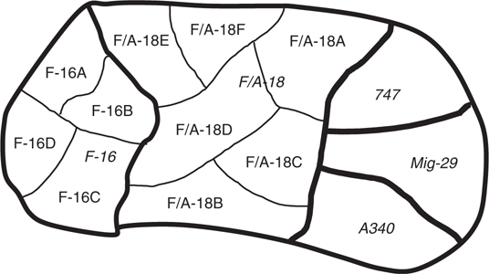
FIGURE 31.19
An f-refinement as a partition refinement.

Images

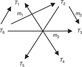
FIGURE 31.20
An example of non-Canonical mapping.

31.7.2 Canonical Mappings

As shown in Figure 31.20, two taxonomies might be related through mappings in more than one way. This shows how sets T₆ and T₃ are related through both the mapping m₃ and the composite mapping m₂*m₁. Since these mappings in general will not be equal for any particular application, a set of canonical mappings must be defined between any two related taxonomies (the canonical mapping from a taxonomy to itself is, of course, the identity mapping). In the case of a collection of taxonomies that are successive refinements, the canonical mappings reflect the hierarchical nature of the taxonomies themselves.

It is conceivable to have multiple canonical mappings between two sets, and to maintain parallel state information for both. This may allow better quality results by combining the two states, since each mapping is an expression of domain information. Thus a state arrived at with one canonical mapping encapsulates background information that the other lacks. More significantly, it is conceivable that the two states might be in conflict. This might indicate an inconsistency in the sensor inputs used to infer the two states, but it also could reflect varying uses or ambiguous interpretations of the observations. The gain from using more than one canonical mapping might or might not be worth the extra complexity.

Images

FIGURE 31.21
Response mapping in a refinement series.

31.7.3 Response Mapping

Response mapping is a way to interpret a response with elements from one taxonomy in terms of another. It also provides a means of interpreting a response with elements from more than one taxonomy in the various referenced taxonomies. Level expansion, which is a case of response mapping among the taxonomies, is of particular interest because of existing sensors that yield a response with elements from both the Type and Class taxonomies (shown by R in Figure 31.21). The objective is to make it possible to maintain parallel states in multiple taxonomies. As each response is received, it is interpreted as described in the following in the taxonomies of interest. The state for each taxonomy is then updated.

This concept is best explained by example. Referring to Figure 31.21, let R be a response from a source of information. It is composed of a set of attributes, potentially from different taxonomies. Let the canonical mapping from taxonomy T_i to taxonomy T_j be m_ij. Each taxonomy potentially has elements that are part of the response (R₁ and R₂ in the figure), as well as elements that are the images, under a canonical mapping, of elements in other taxonomies (m₁₂(R₁), m₂₁(R₂), m₁₃(R₁), m₂₃(R₂)). When the implications of the canonical mappings and the response R have been taken into account, each taxonomy T will experience a response R_T which is the union of the R ∩ T and m_i(R) ∩ T, where m_i is a mapping to T from another taxonomy T_i with elements referenced in R.

31.8 Multihypothesis Structures, Taxonomies, and Recognition of Tactical Elements for CID Fusion

This section extends the previous discussions on the determination of activity, intent, and threat level and develops an extended approach to the JDL model for level 3 SA and CID.

31.8.1 CID in SA and Expansion on the JDL Model

CID in the context of SA is invariably referenced, but far less often is implemented into CID algorithms as an explicit taxonomic process. Hanson and Harper²⁹ demonstrate that situation assessment (for threat refinement) is strongly related to data fusion. A general definition of SA is given by Endsley:³⁰ Situation awareness is the perception of the elements in the environment within a volume of time and space, the comprehension of their meaning, and the projection of their status in the near future. In terms of levels, this definition can be structured in a way analogous to the JDL hierarchy:

Level 1 SA: Perception of the environmental elements. The identification of key elements of events that, in combination, serve to define the situation. This serves to semantically tag key situational elements for higher levels of abstraction in subsequent processing.
Level 2 SA: Comprehension of the current situation. This combines level 1 events into a comprehensive holistic pattern (or tactical situation). This serves to define the current status in operationally relevant terms to support rapid decision making and action.
Level 3 SA: Projection of future status. The projection of the current situation into the future, so as to predict the course of an evolving tactical situation. Time permitting, this supports short-term planning and option evaluation.

A direct comparison of these three levels of SA and JDL data fusion show that the functions are clearly distinct at level 1, since JDL data fusion focuses on the numeric processing of tactical elements to provide identification and tracking, whereas SA focuses on the symbolic processing of these entities, to identify key events in the current situation. At level 2, the definitions are virtually identical to yield the conventional definition of SA (that of generating a holistic pattern of the current situation). At level 3, the SA definition is more general than the pure data fusion definition, since the former also includes projection of ownship */aircraft/battalion/etc., and friendly intent, and capability in addition to threat intent and impact assessment.

Although mission-driven awareness focuses on level 3 SA, due to the desirability of a concurrent multilayered data fusion/SA approach, mission-driven awareness can be used to accelerate level 2 SA and hence focus the fusion process more quickly. Such a benefit may be crucial in the common case of time critical targets of interest.

31.8.2 Recognition of Tactical Elements

Mission-driven awareness allows us to infer from the results of lower level knowledge fusion the mission (or activity) component of CID. Such identification of the mission or activity implies a SA of the decisions made by both sides of an adversarial encounter. This is analogous to the Boyd OODA loop discussed in Section 31.1. This CID capability is not only essential to generate a needed predictive situational awareness (PSA) to minimize fratricide, but is also broadly characteristic of the class of fusion algorithms which can recognize behaviors and project from those behaviors the intent and probable courses of action (CoAs) available to hostile commanders. In short, these fusion algorithms may be represented in the familiar JDL Fusion Model as level 3 fusion to address threat refinement (impact assessment) both predicatively and deductively:

PSA projects CoAs to determine potential impacts (evaluate utility of CoAs to a hostile commander in terms of the impact achieved)
Determination of intent deduces the hostile commander’s intent from the evaluation of the CoAs that best corroborate observed behaviors

Images

FIGURE 31.22
Tactical elements employed by fusion level.

However, these decisions are not generally made at the level of the unit doing the observation (typically a platform such as an aircraft, vehicle, etc.), but rather at a higher decision element that is tasked to perform a given tactical mission. Therefore, to enable decision fusion at an actionable level, recognition of the tactical elements * that represent the decision-level units becomes essential.

This suggestion is based on the observation that although newly developed CID algorithms show great promise for target identification and classification, their utility for determination of intent is limited by their focus on track fusion (JDL levels 1 and 2). Use of a CID architecture structured hierarchically helps implementation of inference processing for level 3 fusion (Figure 31.22 as modified from the 2000 Data and Information Fusion Group).³¹

As may be suggested from Figure 31.22, to reproduce the decision-making process, it is desirable for the decision fusion to be able to recognize and characterize not only individual physical objects (bottom of figure), but also the organizations, events, tactics, objectives, missions, and capabilities (middle to top of figure). Most of these recognition schemes are domain specific and typically either require or at least benefit from use of a priori information (e.g., intelligence).

Accordingly, the JDL model is reorganized in Figure 31.23 to show information flow with the inference level increasing from bottom up. This corresponds loosely to the techniques typically used as discussed in this chapter and shown on the right side of the figure.

Images

FIGURE 31.23
Aggregate of proposed level 0–4 fusion methodologies.

Data structures are displayed on the left side of Figure 31.23. Data structures representative of knowledge fusion as identified in the upper left of the figure include the tactical elements with raid structure and timing, missions, activities, and operational zones. The critical process of generating a situation base, as shown in the center of the figure, represents recognition of tactical elements. The purpose of this section is not to characterize this process so much as to identify the architectural characteristics of a CID structure that would support such a capability. Rather, it is to identify the information and knowledge needed to build such a structure.

Implementation of such an aggregative recognition of tactical elements is facilitated by use of the corresponding architectures for multihypothesis structures and taxonomies for CID. Use of such architectures may in turn facilitate a power to the edge approach to decision making which enables edge units by providing these units with CID information that is structured, traceable, and displayed to the level of recognizable tactical elements for which decisions are made.

The power that would be provided to edge units would be in the form of enhanced CID, earlier CID when contextual cues can discriminate between alternative CID hypotheses, and integration of CoA assessments to evaluate the CID of various threatening elements with the generation of CoAs for mission planning. This information can enable a self-synchronization as described by Alberts and Hayes³² as well as the more obvious support of effects based operations as described by Smith.³³

Determination of a hostile commander’s intent typically requires the representation of his decision-making process. By returning to the dual-view characterized previously that addresses impact assessments in both a predictive and deductive form, one can propose a functional flow as shown in Figure 31.24. In this example, a recognition-primed decision-making (RPD) process is employed as described by Klein.³⁴ As a result, for both forms one can observe the familiar recognition/assessment/evaluation model. For the predictive form at the top of the figure, the system recognizes threatening tactical elements and generates threat assessments and impact predictions. For the deductive form at the bottom of the figure, the system recognizes potential threat intents and generates assessments of intent and their associated CoAs. Acting in tandem, the dual activity model thus proposed provides a useful tool for the determination of intent coupled with the recognition of the critical tactical elements that can be integrated with existing CID assessment tools.

31.9 Conclusions and Future Work

Regardless of the method used to fuse information across the JDL levels, the numerical result of the fusion process (or the confidence in the declaration of Neutral, as an example) does not necessarily provide all of the information necessary to make a decision. This is especially critical for CID where a wrong answer can have disastrous effects. The USS Vincennes incident in July 1988, the Black Hawk shootdown in 1994, and the Patriot Missile battery misidentification in 2003 are all reminders that the context, type, timeliness, quantity, and quality of information must be understood before making a decision. For expansion of work in this area, measures of information value, completeness, and decision cost that complement this multitaxonomic approach for information fusion must be developed. Other future work of interest includes contextual reasoning approaches with extensibility beyond a given domain, realization of the recognition of tactical elements, multiobjective collaborative mission planning and decision making under uncertainty, and PSA integration approaches. Finally, suitable strategies for JDL level 4 and 5 constructs must also be considered, with many approaches available in the literature.

Images

FIGURE 31.24
Potential functional flow for a proposed threat evaluation tool for combat identification.

References

1. McCants, T., CC&D ORD KPP analysis, internal presentation, 22 May 2001.

2. Kebodeaux, C.E., Reducing the Fog of War in the Single Integrated Air Picture through Improved Data Fusion, Thesis to the Air Force Institute of Technology (AFIT), Wright-Patterson AFB, March 2005.

3. White, F.E., Jr., Data Fusion Lexicon, Joint Directors of Laboratories, Technical Panel for C3, Data Fusion Sub-Panel, Naval Ocean Systems Center, San Diego, CA, 1987.

4. Paul, M., Bayesian Belief Networks, Lockheed Martin MS2 internal white paper, August 2002.

5. Chen, G. et al., Game theoretic approach to situational awareness and threat prediction, Proceedings of the 9th International Conference on Information Fusion, Florence, Italy, July, 2006.

6. Hall, D., Lectures in Multisensor Data Fusion and Target Tracking, CD lecture notes section 7.3-272, Artech House, MA, 2001.

7. Schuck, T., Hunter, J. B., and Wilson, D., Multi-hypothesis structures and taxonomies for combat identification fusion, 9th International Command and Control Conference Research and Technology Symposium (ICCRTS), 2004.

8. Schuck, T., A mathematical theory of identification for information fusion, 7th Annual International Command and Control Research and Technology Symposium (ICCRTS), Quebec City, Canada, September 2002.

9. Shannon, C., A mathematical theory of communication, The Bell System Technical Journal, 27, July and October 1948, pp. 379–423 and pp. 623–656.

10. All information associated with Shannon is reproduced or derived from previous Shannon reference.

11. Haak, J., personal communication, March 2002.

12. Schuck, T., Shoemaker, B., and Willey, J., Identification friend-or-foe (IFF) sensor uncertainties, ambiguities, deception, and their application to the multi-source fusion process, IEEE National Aerospace and Electronics Conference (NAECON) 2000, October 2000.

13. Bullard, B. and Dowdy, P., Pulse Doppler Signature of a Rotary-Wing Aircraft, Georgia Tech Research Institute, 1991.

14. Misiurewicz, J., Kulpa, K., and Czekala, Z., Analysis of recorded helicopter echo, radar 97 (Conf. Pub. No. 449), Proceedings of the IEEE 1997, Edinburgh, UK, October 1997, pp. 449–453.

15. Sudano, J., The system probability information content (PIC) relationship to contributing components, combining independent multi-source beliefs, hybrid and pedigree pignistic probabilities, Proceedings of the 5th International Conference on Information Fusion, 2002.

16. Fixsen, D. and Mahler, R., The modified Dempster-Shafer approach to classification, IEEE Transactions on Systems, Man, and Cybernetics-Part A, 27(1), January 1997, pp. 96–104.

17. Fister, T. and Mitchell, R., Modified Dempster-Shafer with entropy based belief body compression, Proceedings of the 1994 Joint Service Combat Identification Systems Conference (CISC), Naval Postgraduate School, CA, August 1994.

18. Sudano, J., Pignistic probability transforms for mixes of low and high probability events, 4th International Conference on Information Fusion, Montreal, Canada, August 2001.

19. Powell, M., Decision and Risk Analysis for Complex Systems, Course at the Stevens Institute of Technology, Hoboken, NJ, 2006.

20. Haspert, K., Optimum ID Sensor Fusion for Multiple Target Types, Institute for Defense Analysis Document D-2451, March 2000.

21. Athena multi-source integration—systems engineering team (MSI-SET) final report, 1998.

22. Stevens, M., Secondary Surveillance Radar, Artech House, MA, 1988.

23. Shoemaker, W.B., IFF on the AN/SPS-40 Multipath Diagram, USNS Capable testing, 1998.

24. Lothes, R.N., Szymanski, M.B., and Wiley, R.G., Radar Vulnerability to Jamming, Artech House, MA, 1990.

25. Alberts, D. et al., Understanding Information Age Warfare, DOD Command and Control Research Program (CCRP), CCRP Press, Washington DC, July 2002.

26. Friesel, M., A Bernoulli Analysis for Multiple Observations of a Single Object, Lockheed Martin internal document, 2004.

27. Sudano, J., Equivalence between belief theories and naïve bayesian fusion for systems with independent evidential data: Part 1 the theory, Proceedings of the Sixth International Conference on Information Fusion, July 2003.

28. Schuck, T., Hunter, J., and Wilson, D., Multi-hypothesis structures and taxonomies for combat identification fusion, Proceedings of the IEEE Aerospace Conference, Big Sky, MT, March 2004.

29. Hanson, M.L. and Harper, K.A., An intelligent agent for supervisory control of teams of uninhabited combat air vehicles (UCAVs), Unmanned Systems 2000 Conference, July 11–13, 2000.

30. Endsley, M.R., Toward a theory of situation awareness in dynamic systems, Human Factors, 37(1), 1995, pp. 32–64.

31. Data & Information Group, Data & information fusion: Status of U.S. data & information fusion, Fusion 2000 Conference, Paris, France, 10 July 2000.

32. Alberts, D.S. and Hayes, R.E., Power to the Edge, DOD Command and Control Research Program (CCRP), CCRP Press, Washington DC, June 2003.

33. Smith E.A., Effects Based Operations: Applying Network Centric Warfare in Peace, Crisis and War, DOD Command and Control Research Program (CCRP), CCRP Press, Washington DC, 2002.

34. Klein, G.A., Naturalistic decision making: Implications for design, Gateway, 5(1), 1994, pp. 6–7, also Recognition-primed decisions, Advances in Man-Machine Systems Research, 5, 1989, pp. 47–92.

* Portions reprinted, with permission, from Proceedings of the IEEE National Aerospace and Electronics Conference (NAECON) 2000, c October 2000; Proceedings of the 6th International Conference on Information Fusion, c July 2003; and Proceedings of the IEEE Aerospace Conference, c March, 2004.

† The author’s affiliation with the MITRE Corporation is provided only for identification purpose and is not intended to convey or imply MITRE’s concurrence with, or support for, the positions, opinions, or viewpoints expressed by the author.

* Hereto described as battlespace objects or simply objects.

† The platform or node attempting to identify a detected object.

* A measurement of information entropy, in a CID context, can be described as a means to capturing and quantifying the amount of information, choice, and uncertainty associated with the output of a sensor source and a CID fusion process.

† It is described in other chapters.

* The OODA (Observe-Orient-Decide-Act) was first described by Col. J.R. Boyd in the 1950’s and is described by T.A. Hightower in “Boyd’s O.O.D.A. Loop and How We Use It.” (http://www.tacticalresonse.com/d/node/226).

* The SCI and FI-B curves shown here are based on the results from algorithms that are still under development. These will be presented in later publications.

* Ownship can refer to one’s self, platform, organization, etc.

* Often an organizational entity such as an armored column, flight of aircraft, convoy of vehicles, terrorist cell, and so on.

..................Content has been hidden....................

You can't read the all page of ebook, please click here login for view all page.

Table of Contents for
31 Developing Information Fusion Methods for Combat Identification

31

*Developing Information Fusion Methods for Combat Identification**

31.1 Introduction

31.2 Mapping CID to JDL Levels

31.2.1 Multihypothesis Structures

31.2.1.1 JDL Level 1 Structures

31.2.1.2 JDL Level 2 Structures

31.2.1.3 JDL Level 3 Structures

31.3 CID Information and Information Theory

31.3.1 The Identification System

31.3.2 Forming the Identification Vector

31.3.3 Choice, Uncertainty, and Entropy for Identification

31.3.3.1 Example of Identification Information Measurement

31.4 Understanding IFF Sensor Uncertainties

31.5 Information Properties as a Means to Define CID Fusion Methodologies

31.6 Fusion Methods

31.6.1 Modified Dempster–Shafer Approach

31.6.2 Information Fusion Sets

31.6.2.1 Bayesian and Orthodox D-S Results

31.6.3 Results and Discussion

31.7 Multihypothesis Structures and Taxonomies for CID Fusion

31.7.1 Taxonomic Relationships Defined

31.7.2 Canonical Mappings

31.7.3 Response Mapping

31.8 Multihypothesis Structures, Taxonomies, and Recognition of Tactical Elements for CID Fusion

31.8.1 CID in SA and Expansion on the JDL Model

31.8.2 Recognition of Tactical Elements

31.9 Conclusions and Future Work

References

Table of Contents for 31 Developing Information Fusion Methods for Combat Identification

Create new playlist

Sign In

Sign Up

Table of Contents for
31 Developing Information Fusion Methods for Combat Identification