
Chapter One
Positive Matrices
We begin with a quick review of some of the basic properties of positive matrices. This will serve as a warmup and orient the reader to the line of thinking followed through the book.
1.1 CHARACTERIZATIONS
Let ![]() be the n-dimensional Hilbert space
be the n-dimensional Hilbert space ![]() . The inner product between two vectors x
and y is written as
. The inner product between two vectors x
and y is written as ![]() or as x∗y. We adopt the convention that the inner product is
conjugate linear in the first variable and linear in the second. We denote by
or as x∗y. We adopt the convention that the inner product is
conjugate linear in the first variable and linear in the second. We denote by ![]() the
space of all linear operators on
the
space of all linear operators on ![]() , and by
, and by ![]() or simply
or simply ![]() the space of n × n matrices
with complex entries. Every element A of
the space of n × n matrices
with complex entries. Every element A of ![]() can be identified with its matrix with
respect to the standard basis {ej} of
can be identified with its matrix with
respect to the standard basis {ej} of ![]() . We use the symbol A for this matrix as well.
We say A is positive semidefinite if
. We use the symbol A for this matrix as well.
We say A is positive semidefinite if
and positive definite if, in addition,
A positive semidefinite matrix is positive definite if and only if it is invertible.
For the sake of brevity, we use the term positive matrix for a positive semidefinite, or a positive definite, matrix. Sometimes, if we want to emphasize that the matrix is positive definite, we say that it is strictly positive. We use the notation A ≥ O to mean that A is positive, and A > O to mean it is strictly positive.
There are several conditions that characterize positive matrices. Some of them are listed below.
(i) A is positive if and only if it is Hermitian (A = A∗) and all its eigenvalues are nonnegative. A is strictly positive if and only if all its eigenvalues are positive.
(ii) A is positive if and only if it is Hermitian and all its principal minors are nonnegative. A is strictly positive if and only if all its principal minors are positive.
(iii) A is positive if and only if A = B∗B for some matrix B. A is strictly positive if and only if B is nonsingular.
(iv) A is positive if and only if A = T∗T for some upper triangular matrix T. Further, T can be chosen to have nonnegative diagonal entries. If A is strictly positive, then T is unique. This is called the Cholesky decomposition of A. A is strictly positive if and only if T is nonsingular.
(v) A is positive if and only if A = B2 for some positive matrix B. Such a B is unique. We write B = A1/2 and call it the (positive) square root of A. A is strictly positive if and only if B is strictly positive.
(vi)
A is positive if and only if there exist x1, . . . , xn in ![]() such that
such that
A is strictly positive if and only if the vectors xj, 1 ≤ j ≤ n, are linearly independent.
A proof of the sixth characterization is outlined below. This will serve the purpose of setting up some notations and of introducing an idea that will be often used in the book.
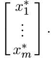
We think of elements of ![]() as column vectors. If x1, . . . , xm are such vectors we
write [x1, . . . , xm] for the n × m matrix whose columns are x1, . . . , xm. The
adjoint of this matrix is written as
as column vectors. If x1, . . . , xm are such vectors we
write [x1, . . . , xm] for the n × m matrix whose columns are x1, . . . , xm. The
adjoint of this matrix is written as
This is an m × n matrix whose rows are the (row) vectors x∗1, . . . , x∗m. We use the symbol [[aij]] for a matrix with i, j entry aij.
Now if x1, . . . , xn are elements of ![]() , then
, then
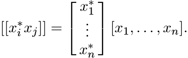
So, this matrix is positive (being of the form B∗B). This shows that the condition (1.3) is sufficient for A to be positive. Conversely, if A is positive, we can write
If we choose xj = A1/2ej, we get (1.3).
1.1.1 Exercise
Let x1, . . . , xm be any m vectors in any Hilbert space. Then the m×m matrix
is positive. It is strictly positive if and only if x1, . . . , xm are linearly independent.
The matrix (1.4) is called the Gram matrix associated with the vectors x1, . . . , xm.
1.1.2 Exercise
Let λ1, . . . , λm be positive numbers. The m×m matrix A with entries
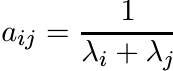 (1.5)
(1.5)is called the Cauchy matrix (associated with the numbers λj). Note that
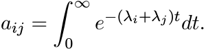 (1.6)
(1.6)
Let fi(t) = e−λit, 1 ≤ i ≤ m. Then fi ∈ L2([0, ∞)) and ![]() . This shows that A is positive.
. This shows that A is positive.
More generally, let λ1, . . . , λm be complex numbers whose real parts are positive. Show that the matrix A with entries
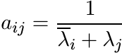
is positive.
1.1.3 Exercise
Let µ be a finite positive measure on the interval [−π, π]. The numbers
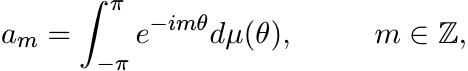 (1.7)
(1.7)are called the Fourier-Stieltjes coefficients of µ. For any n = 1, 2, . . . , let A be the n × n matrix with entries
Then A is positive.
Note that the matrix A has the form
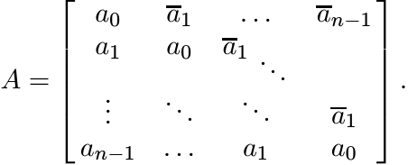 (1.9)
(1.9)One special feature of this matrix is that its entries are constant along the diagonals parallel to the main diagonal. Such a matrix is called a Toeplitz matrix. In addition, A is Hermitian.
A doubly infinite sequence {am : m ∈ ![]() } of complex numbers is said to be a positive
definite sequence if for each n = 1, 2, . . . , the n × n matrix (1.8) constructed
from this sequence is positive. We have seen that the Fourier-Stieltjes coefficients
of a finite positive measure on [−π, π] form a positive definite sequence. A basic
theorem of harmonic analysis called the Herglotz theorem says that, conversely, every
positive definite sequence is the sequence of Fourier-Stieltjes coefficients of a
finite positive measure µ. This theorem is proved in Chapter 5.
} of complex numbers is said to be a positive
definite sequence if for each n = 1, 2, . . . , the n × n matrix (1.8) constructed
from this sequence is positive. We have seen that the Fourier-Stieltjes coefficients
of a finite positive measure on [−π, π] form a positive definite sequence. A basic
theorem of harmonic analysis called the Herglotz theorem says that, conversely, every
positive definite sequence is the sequence of Fourier-Stieltjes coefficients of a
finite positive measure µ. This theorem is proved in Chapter 5.
1.2 SOME BASIC THEOREMS
Let A be a positive operator on ![]() . If X is a linear operator from a Hilbert space
. If X is a linear operator from a Hilbert space
![]() into
into ![]() , then the operator X∗AX on
, then the operator X∗AX on ![]() is also positive. If X is an invertible opertator,
and X∗AX is positive, then A is positive.
is also positive. If X is an invertible opertator,
and X∗AX is positive, then A is positive.
Let A, B be operators on ![]() . We say that A is congruent to B, and write A ∼ B, if there
exists an invertible operator X on
. We say that A is congruent to B, and write A ∼ B, if there
exists an invertible operator X on ![]() such that B = X∗AX. Congruence is an equivalence
relation on
such that B = X∗AX. Congruence is an equivalence
relation on ![]() . If X is unitary, we say A is unitarily equivalent to B, and write A
≃ B.
. If X is unitary, we say A is unitarily equivalent to B, and write A
≃ B.
If A is Hermitian, the inertia of A is the triple of nonnegative integers
where π(A), ζ(A), ν(A) are the numbers of positive, zero, and negative eigenvalues of A (counted with multiplicity).
Sylvester’s law of inertia says that In(A) is a complete invariant for congruence on the set of Hermitian matrices; i.e., two Hermitian matrices are congruent if and only if they have the same inertia. This can be proved in different ways. Two proofs are outlined below.
1.2.1 Exercise
Let ![]() be the eigenvalues of the Hermitian matrix A arranged in decreasing order.
By the minimax principle (MA, Corollary III.1.2)
be the eigenvalues of the Hermitian matrix A arranged in decreasing order.
By the minimax principle (MA, Corollary III.1.2)
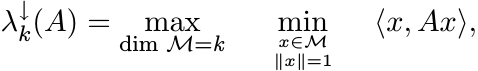
where ![]() stands for a subspace of
stands for a subspace of ![]() and dim
and dim ![]() for its dimension. If X is an invertible
operator, then dim
for its dimension. If X is an invertible
operator, then dim ![]() . Use this to prove that any two congruent Hermitian matrices
have the same inertia.
. Use this to prove that any two congruent Hermitian matrices
have the same inertia.
1.2.2 Exercise
Let A be a nonsingular Hermitian matrix and let B = X∗AX, where X is any nonsingular matrix. Let X have the polar decomposition X = UP, where U is unitary and P is strictly positive. Let
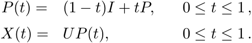
Then P(t) is strictly positive, and X(t) nonsingular. We have X(0) = U, and X(1) = X. Thus X(t)∗AX(t) is a continuous curve in the space of nonsingular matrices joining U∗AU and X∗AX. The eigenvalues of X(t)∗AX(t) are continuous curves joining the eigenvalues of U∗AU (these are the same as the eigenvalues of A) and the eigenvalues of X∗AX = B. [MA, Corollary VI.1.6]. These curves never touch the point zero. Hence
i.e., A and B have the same inertia.
Modify this argument to cover the case when A is singular. (Then
ζ(A) = ζ(B). Consider A ± εI.)
1.2.3 Exercise
Show that a Hermitian matrix A is congruent to the diagonal matrix diag (1, . . . , 1, 0, . . . , 0, −1, . . . , −1), in which the entries 1, 0, −1 occur π(A), ζ(A), and ν(A) times on the diagonal. Thus two Hermitian matrices with the same inertia are congruent.
Two Hermitian matrices are unitarily equivalent if and only if they have the same eigenvalues (counted with multiplicity).
Let ![]() be a subspace of
be a subspace of ![]() and let P be the orthogonal projection onto
and let P be the orthogonal projection onto ![]() . If we choose
an orthonormal basis in which
. If we choose
an orthonormal basis in which ![]() is spanned by the first k vectors, then we can write
an operator A on
is spanned by the first k vectors, then we can write
an operator A on ![]() as a block matrix
as a block matrix
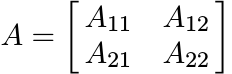
and
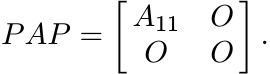
If V is the injection of ![]() into
into ![]() , then V ∗AV = A11. We say that A11 is the compression
of A to
, then V ∗AV = A11. We say that A11 is the compression
of A to ![]() .
.
If A is positive, then all its compressions are positive. Thus all principal submatrices of a positive matrix are positive. Conversely, if all the principal subdeterminants of A are nonnegative, then the coefficients in the characteristic polynomial of A alternate in sign. Hence, by the Descartes rule of signs A has no negative root.
The following exercise says that if all the leading subdeterminants of a Hermitian matrix A are positive, then A is strictly positive. Positivity of other principal minors follows as a consequence.
Let A be Hermitian and let B be its compression to an (n − k)-dimensional subspace. Then Cauchy’s interlacing theorem [MA, Corollary III.1.5] says that
1.2.4 Exercise
(i) If A is strictly positive, then all its compressions are strictly positive.
(ii) For 1 ≤ j ≤ n let A[j] denote the j × j block in the top left corner of the matrix of A. Call this the leading j × j submatrix of A, and its determinant the leading j × j subdeterminant. Show that A is strictly positive if and only if all its leading subdeterminants are positive. [Hint: use induction and Cauchy’s interlacing theorem.]
The example ![]() shows that nonnegativity of the two leading subdeterminants is not adequate
to ensure positivity of A.
shows that nonnegativity of the two leading subdeterminants is not adequate
to ensure positivity of A.
We denote by ![]() the tensor product of two operators A and B (acting possibly on different
Hilbert spaces
the tensor product of two operators A and B (acting possibly on different
Hilbert spaces ![]() and
and ![]() ). If A, B are positive, then so is
). If A, B are positive, then so is ![]() .
.
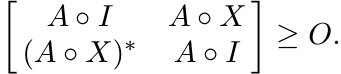
If A, B are n×n matrices we write A◦B for their entrywise product; i.e., for the
matrix whose i, j entry is aijbij. We will call this the Schur product of A and B.
It is also called the Hadamard product. If A and B are positive, then so is A◦ B.
One way of seeing this is by observing that A ◦ B is a principal submatrix of ![]() .
.
1.2.5 Exercise
Let A, B be positive matrices of rank one. Then there exist vectors x, y such that A = xx∗, B = yy∗. Show that A ◦ B = zz∗, where z is the vector x ◦ y obtained by taking entrywise product of the coordinates of x and y. Thus A ◦ B is positive. Use this to show that the Schur product of any two positive matrices is positive.
If both A, B are Hermitian, or positive, then so is A + B. Their product AB is, however, Hermitian if and only if A and B commute. This condition is far too restrictive. The symmetrized product of A, B is the matrix
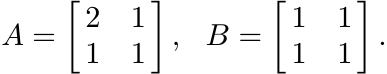
If A, B are Hermitian, then S is Hermitian. However, if A, B are positive, then S need not be positive. For example, the matrices
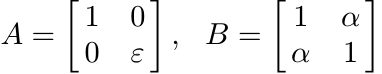
are positive if ε > 0 and 0 < α < 1, but S is not positive when ε is close to zero and α is close to 1. In view of this it is, perhaps, surprising that if S is positive and A strictly positive, then B is positive. Three different proofs of this are outlined below.
1.2.6 Proposition
Let A, B be Hermitian and suppose A is strictly positive. If the symmetrized product S = AB + BA is positive (strictly positive), then B is positive (strictly positive).
Proof. Choose an orthonormal basis in which B is diagonal; B = diag(β1, . . . , βn). Then sii = 2βiaii. Now observe that the diagonal entries of a (strictly) positive matrix are (strictly) positive. ■
1.2.7 Exercise
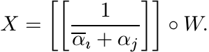
Choose an orthonormal basis in which A is diagonal with entries α1, α2, . . . , αn, on its diagonal. Then note that S is the Schur product of B with the matrix [[αi + αj]]. Hence B is the Schur product of S with the Cauchy matrix [[1/(αi + αj)]]. Since this matrix is positive, it follows that B is positive if S is.
1.2.8 Exercise
If S > O, then for every nonzero vector x
Suppose Bx = βx with β ≤ 0. Show that ![]() . Conclude that B > O.
. Conclude that B > O.
An amusing corollary of Proposition 1.2.6 is a simple proof of the operator monotonicity
of the map ![]() on positive matrices.
on positive matrices.
If A, B are Hermitian, we say that A ≥ B if A− B ≥ O; and A > B if A − B > O.
1.2.9 Proposition
If A, B are positive and A > B, then A1/2 > B1/2.
Proof. We have the identity
 (1.13)
If X, Y are strictly positive then X + Y is strictly positive. So, if X2 − Y 2 is positive, then X − Y is positive by Proposition 1.2.6. ■
Recall that if A ≥ B, then we need not always have A2 ≥ B2; e.g., consider the matrices
Proposition 1.2.6 is related to the study of the Lyapunov equation, of great importance in differential equations and control theory. This is the equation (in matrices)
It is assumed that the spectrum of A is contained in the open right half-plane. The matrix A is then called positively stable. It is well known that in this case the equation (1.14) has a unique solution. Further, if W is positive, then the solution X is also positive.
1.2.10 Exercise
Suppose A is diagonal with diagonal entries α1, . . . , αn. Then the solution of (1.14) is
Use Exercise 1.1.2 to see that if W is positive, then so is X. Now suppose A = TDT−1, where D is diagonal. Show that again the solution X is positive if W is positive. Since diagonalisable matrices are dense in the space of all matrices, the same conclusion can be obtained for general positively stable A.
The solution X to the equation (1.14) can be represented as the integral
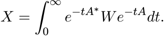 (1.15)
The condition that A is positively stable ensures that this integral is convergent. It is easy to see that X defined by (1.15) satisfies the equation (1.14). From this it is clear that if W is positive, then so is X.
Now suppose A is any matrix and suppose there exist positive matrices X and W such that the equality (1.14) holds. Then if Au = αu, we have
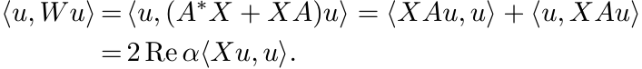
This shows that A is positively stable.
1.2.11 Exercise
The matrix equation
is called the Stein equation or the discrete time Lyapunov equation. It is assumed that the spectrum of F is contained in the open unit disk. Show that in this case the equation has a unique solution given by
 (1.17)
From this it is clear that if W is positive, then so is X. Another proof of this
fact goes as follows. To each point β in the open unit disk there corresponds a unique
point α in the open right half plane given by ![]() . Suppose F is diagonal with diagonal
entries β1, . . . , βn. Then the solution of (1.16) can be written as
. Suppose F is diagonal with diagonal
entries β1, . . . , βn. Then the solution of (1.16) can be written as
Use the correspondence between β and α to show that
Now use Exercise 1.2.10.
If F is any matrix such that the equality (1.16) is satisfied by some positive matrices X and W, then the spectrum of F is contained in the unit disk.
1.2.12 Exercise
Let A, B be strictly positive matrices such that A ≥ B. Show that A−1 ≤ B−1. [Hint: If A ≥ B, then I ≥ A−1/2BA−1/2.]
1.2.13 Exercise
The quadratic equation
is called a Riccati equation. If B is positive and A strictly positive, then this equation has a positive solution. Conjugate the two sides of the equation by A1/2, take square roots, and then conjugate again by A−1/2 to see that
is a solution. Show that this is the only positive solution.
1.3 BLOCK MATRICES
Now we come to a major theme of this book. We will see that 2 × 2 block matrices
![]() can play a remarkable—almost magical—role in the study of positive matrices.
can play a remarkable—almost magical—role in the study of positive matrices.
In this block matrix the entries A, B, C, D are n × n matrices. So, the big matrix
is an element of ![]() , or, of
, or, of ![]() . As we proceed we will see that several properties of
A can be obtained from those of a block matrix in which A is one of the entries.
Of special importance is the connection this establishes between positivity (an algebraic
property) and contractivity (a metric property).
. As we proceed we will see that several properties of
A can be obtained from those of a block matrix in which A is one of the entries.
Of special importance is the connection this establishes between positivity (an algebraic
property) and contractivity (a metric property).
Let us fix some notations. We will write A = UP for the polar decomposition of A. The factor U is unitary and P is positive; we have P = (A∗A)1/2. This is called the positive part or the absolute value of A and is written as |A|. We have A∗ = PU∗, and
A is said to be normal if AA∗ = A∗A. This condition is equivalent to UP = PU; and to the condition |A| = |A∗|.
We write A = USV for the singular value decomposition (SVD) of A. Here U and V are unitary and S is diagonal with nonnegative diagonal entries s1(A) ≥ · · · ≥ sn(A). These are the singular values of A (the eigenvalues of |A|).
The symbol ||A|| will always denote the norm of A as a linear operator on the Hilbert
space ![]() ; i.e.,
; i.e.,
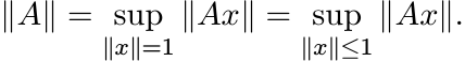
It is easy to see that ||A|| = s1(A).
Among the important properties of this norm are the following:
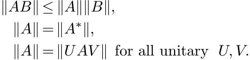 (1.18)
This last property is called unitary invariance. Finally
There are several other norms on ![]() that share the three properties (1.18). It is the
condition (1.19) that makes the operator norm || · || very special.
that share the three properties (1.18). It is the
condition (1.19) that makes the operator norm || · || very special.
We say A is contractive, or A is a contraction, if ||A|| ≤ 1.
1.3.1 Proposition
The operator A is contractive if and only if the operator ![]() is positive.
is positive.
Proof. What does the proposition say when ![]() is one-dimensional? It just says that
if a is a complex number, then |a| ≤ 1 if and only if the 2 × 2 matrix
is one-dimensional? It just says that
if a is a complex number, then |a| ≤ 1 if and only if the 2 × 2 matrix ![]() is positive.
The passage from one to many dimensions is made via the SVD. Let A = USV . Then
is positive.
The passage from one to many dimensions is made via the SVD. Let A = USV . Then
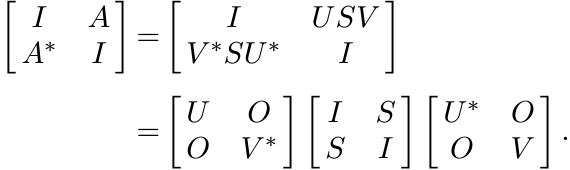
This matrix is unitarily equivalent to ![]() , which in turn is unitarily equivalent to
the direct sum
, which in turn is unitarily equivalent to
the direct sum
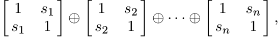
where s1, . . . , sn are the singular values of A. These 2 × 2 matrices are all positive if and only if s1 ≤ 1 (i.e.,||A|| ≤ 1). ■
1.3.2 Proposition
Let A, B be positive. Then the matrix ![]() is positive if and only if X = A1/2KB1/2 for
some contraction K.
is positive if and only if X = A1/2KB1/2 for
some contraction K.
Proof. Assume first that A, B are strictly positive. This allows us to use the congruence

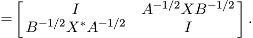
Let K = A−1/2XB−1/2. Then by Proposition 1.3.1 this block matrix is positive if and only if K is a contraction. This proves the proposition when A, B are strictly positive. The general case follows by a continuity argument. ■
It follows from Proposition 1.3.2 that if ![]() is positive, then the range of X is a
subspace of the range of A, and the range of X∗ is a subspace of the range of B.
The rank of X cannot exceed either the rank of A or the rank of B.
is positive, then the range of X is a
subspace of the range of A, and the range of X∗ is a subspace of the range of B.
The rank of X cannot exceed either the rank of A or the rank of B.
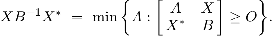
1.3.3 Theorem
Let A, B be strictly positive matrices. Then the block matrix ![]() is positive if and
only if A ≥ XB−1X∗.
is positive if and
only if A ≥ XB−1X∗.
Proof. We have the congruence
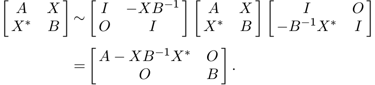
Clearly, this last matrix is positive if and only if A ≥ XB−1X∗. ■
Second proof. We have A ≥ XB−1X∗ if and only if
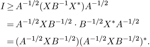
This is equivalent to saying ||A−1/2XB−1/2|| ≤ 1, or X = A1/2KB1/2 where ||K|| ≤ 1. Now use Proposition 1.3.2. ■
1.3.4 Exercise
Show that the condition A ≥ XB−1X∗ in the theorem cannot be replaced by A ≥ X∗B−1X
(except when ![]() is one dimensional!).
is one dimensional!).
1.3.5 Exercise
Let A, B be positive but not strictly positive. Show that Theorem 1.3.3 is still valid if B−1 is interpreted to be the Moore-Penrose inverse of B.
1.3.6 Lemma
The matrix A is positive if and only if ![]() is positive.
is positive.
Proof. We can write
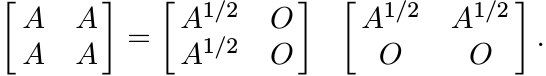
1.3.7 Corollary
Let A be any matrix. Then the matrix ![]() is positive.
is positive.
Proof. Use the polar decomposition A = UP to write
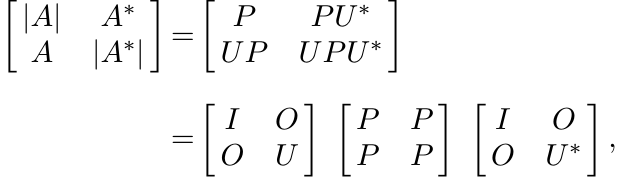
and then use the lemma. ■
1.3.8 Corollary
If A is normal, then ![]() is positive.
is positive.
1.3.9 Exercise
Show that (when n ≥ 2) this is not always true for nonnormal matrices.
1.3.10 Exercise
If A is strictly positive, show that ![]() is positive (but not strictly positive.)
is positive (but not strictly positive.)
Theorem 1.3.3, the other propositions in this section, and the ideas used in their proofs will occur repeatedly in this book. Some of their power is demonstrated in the next sections.
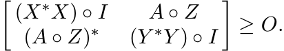
1.4 NORM OF THE SCHUR PRODUCT
Given A in Mn, let SA be the linear map on Mn defined as
where A◦ X is the Schur product of A and X. The norm of this linear operator is, by definition,
 (1.21)
Since
we have
Finding the exact value of ||SA|| is a difficult problem in general. Some special cases are easier.
1.4.1 Theorem (Schur)
If A is positive, then
Proof. Let ||X|| ≤ 1. Then by Proposition 1.3.1 ![]() . By Lemma 1.3.6
. By Lemma 1.3.6 ![]() . Hence the Schur
product of these two block matrices is positive; i.e,
. Hence the Schur
product of these two block matrices is positive; i.e,
So, by Proposition 1.3.2, ||A◦ X|| ≤ ||A◦ I|| = max aii. Thus ||SA|| = max aii. ■
1.4.2 Exercise
If U is unitary, then ||SU|| = 1. [Hint: ![]() is doubly stochastic, and hence, has norm
1.]
is doubly stochastic, and hence, has norm
1.]
For each matrix X, let
||X||c = maximum of the Euclidean norms of columns of X. (1.25)
This is a norm on Mn, and
1.4.3 Theorem
Let A be any matrix. Then
Proof. Let A = X∗Y . Then
 (1.28)
Now if Z is any matrix with ||Z|| ≤ 1, then ![]() . So, the Schur product of this with
the positive matrix in (1.28) is positive; i.e.,
. So, the Schur product of this with
the positive matrix in (1.28) is positive; i.e.,
Hence, by Proposition 1.3.2
Thus ||SA|| ≤ ||X||c||Y ||c. ■
In particular, we have
which is an improvement on (1.23).
In Chapter 3, we will prove a theorem of Haagerup (Theorem 3.4.3) that says the two sides of (1.27) are equal.
1.5 MONOTONICITY AND CONVEXITY
Let ![]() be the space of self-adjoint (Hermitian) operators on
be the space of self-adjoint (Hermitian) operators on ![]() . This is a real vector
space. The set
. This is a real vector
space. The set ![]() of positive operators is a convex cone in this space. The set of
strictly positive operators is denoted by
of positive operators is a convex cone in this space. The set of
strictly positive operators is denoted by ![]() . It is an open set in
. It is an open set in ![]() and is a convex
cone. If f is a map of
and is a convex
cone. If f is a map of ![]() into itself, we say f is convex if
into itself, we say f is convex if
for all ![]() and for 0 ≤ α ≤ 1. If f is continuous, then f is convex if and only if
and for 0 ≤ α ≤ 1. If f is continuous, then f is convex if and only if
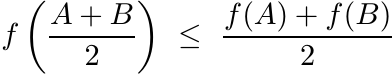 (1.31)
for all A, B.
We say f is monotone if f(A) ≥ f(B) whenever A ≥ B.
The results on block matrices in Section 1.3 lead to easy proofs of the convexity and monotonicity of several functions. Here is a small sampler.
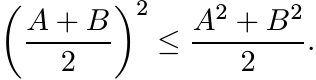
Let A, B > O. By Exercise 1.3.10
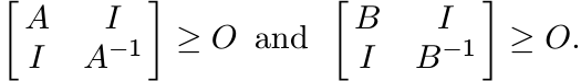 (1.32)
Hence,
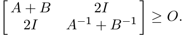
By Theorem 1.3.3 this implies
or
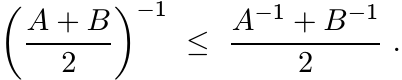 (1.33)
Thus the map ![]() is convex on the set of positive matrices.
is convex on the set of positive matrices.
Taking the Schur product of the two block matrices in (1.32) we get
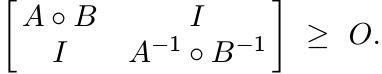
So, by Theorem 1.3.3
The special choice B = A−1 gives
But a positive matrix is larger than its inverse if and only if it is larger than I. Thus we have the inequality
known as Fiedler’s inequality.
1.5.1 Exercise
Use Theorem 1.3.3 to show that the map ![]() from
from ![]() into
into ![]() is jointly convex, i.e.,
is jointly convex, i.e.,

In particular, this implies that the map ![]() on
on ![]() is convex (a fact we have proved earlier),
and that the map
is convex (a fact we have proved earlier),
and that the map ![]() on
on ![]() is convex. The latter statement can be proved directly: for
all Hermitian matrices A and B we have the inequality
is convex. The latter statement can be proved directly: for
all Hermitian matrices A and B we have the inequality
1.5.2 Exercise
Show that the map ![]() is not convex on 2 × 2 positive matrices.
is not convex on 2 × 2 positive matrices.
1.5.3 Corollary
The map ![]() is jointly concave on
is jointly concave on ![]()
![]() . It is monotone increasing in the variables A, B.
. It is monotone increasing in the variables A, B.
In particular, the map ![]() on
on ![]() is monotone (a fact we proved earlier in Exercise 1.2.12).
is monotone (a fact we proved earlier in Exercise 1.2.12).
1.5.4 Proposition
Let B > O and let X be any matrix. Then
 (1.36)
Proof. This follows immediately from Theorem 1.3.3. ■
1.5.5 Corollary
Let A, B be positive matrices and X any matrix. Then
 (1.37)
Proof. Use Proposition 1.5.4. ■
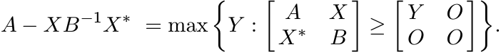
Extremal representations such as (1.36) and (1.37) are often used to derive matrix inequalities. Most often these are statements about convexity of certain maps. Corollary 1.5.5, for example, gives useful information about the Schur complement, a concept much used in matrix theory and in statistics.
Given a block matrix ![]() the Schur complement of A22 in A is the matrix
the Schur complement of A22 in A is the matrix
The Schur complement of A11 is the matrix obtained by interchanging the indices 1 and 2 in this definition. Two reasons for interest in this object are given below.
1.5.6 Exercise
Show that
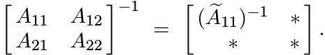
1.5.7 Exercise
If A is invertible, then the top left corner of the block matrix A−1 is ![]() ; i.e.,
; i.e.,
Corollary 1.5.3 says that on the set of positive matrices (with a block decomposition)
the Schur complement is a concave function. Let us make this more precise. Let ![]() be
an orthogonal decomposition of H. Each operator A on H can be written as A =
be
an orthogonal decomposition of H. Each operator A on H can be written as A = ![]() with
respect to this decomposition. Let
with
respect to this decomposition. Let ![]() . Then for all strictly positive operators A and
B we have
. Then for all strictly positive operators A and
B we have
The map ![]() is positively homogenous; i.e., P(αA) = αP(A) for all positive numbers α.
It is also monotone in A.
is positively homogenous; i.e., P(αA) = αP(A) for all positive numbers α.
It is also monotone in A.
We have seen that while the function f(A) = A2 is convex on the space of positive matrices, the function f(A) = A3 is not; and while the function f(A) = A1/2 is monotone on the set of positive matrices, the function f(A) = A2 is not. Thus the following theorems are interesting.
1.5.8 Theorem
The function f(A) = Ar is convex on ![]() for 1 ≤ r ≤ 2.
for 1 ≤ r ≤ 2.
Proof. We give a proof that uses Exercise 1.5.1 and a useful integral representation of Ar. For t > 0 and 0 < r < 1, we have (from one of the integrals calculated via contour integration in complex analysis)
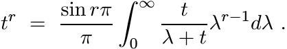
The crucial feature of this formula that will be exploited is that we can represent tr as
 (1.39)
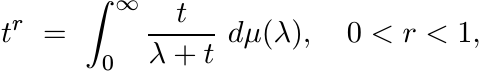
where µ is a positive measure on (0, ∞). Multiplying both sides by t, we have
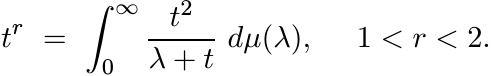
Thus for positive operators A, and for 1 < r < 2,
By Exercise 1.5.1 the integrand is a convex function of A for each λ > 0. So the integral is also convex. ■
1.5.9 Theorem
The function f(A) = Ar is monotone on ![]() for 0 ≤ r ≤ 1.
for 0 ≤ r ≤ 1.
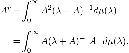
Proof. For each λ > 0 we have A(λ + A)−1 = (λA−1 + I)−1. Since the map ![]() is monotonically
decreasing (Exercise 1.2.12), the function fλ(A) = A(λ + A)−1 is monotonically increasing
for each λ > 0. Now use the integral representation (1.39) as in the preceding
proof. ■
is monotonically
decreasing (Exercise 1.2.12), the function fλ(A) = A(λ + A)−1 is monotonically increasing
for each λ > 0. Now use the integral representation (1.39) as in the preceding
proof. ■
1.5.10 Exercise
Show that the function f(A) = Ar is convex on ![]() for −1 ≤ r ≤ 0. [Hint: For −1 <
r < 0 we have
for −1 ≤ r ≤ 0. [Hint: For −1 <
r < 0 we have
Use the convexity of the map f(A) = A−1.]
1.6 SUPPLEMENTARY RESULTS AND EXERCISES
Let A and B be Hermitian matrices. If there exists an invertible matrix X such that X∗AX and X∗BX are diagonal, we say that A and B are simultaneously congruent to diagonal matrices (or A and B are simultaneously diagonalizable by a congruence). If X can be chosen to be unitary, we say A and B are simultaneously diagonalizable by a unitary conjugation.
Two Hermitian matrices are simultaneously diagonalizable by a unitary conjugation if and only if they commute. Simultaneous congruence to diagonal matrices can be achieved under less restrictive conditions.
1.6.1 Exercise
Let A be a strictly positive and B a Hermitian matrix. Then A and B are simultaneously congruent to diagonal matrices. [Hint: A is congruent to the identity matrix.]
Simultaneous diagonalization of three matrices by congruence, however, again demands severe restrictions. Consider three strictly positive matrices I, A1 and A2. Suppose X is an invertible matrix such that X∗X is diagonal. Then X = UΛ where U is unitary and Λ is diagonal and invertible. It is easy to see that for such an X, X∗A1X and X∗A2X both are diagonal if and only if A1 and A2 commute.
If A and B are Hermitian matrices, then the inequality AB + BA ≤ A2 + B2 is always true. It follows that if A and B are positive, then
Using the monotonicity of the square root function we see that
In other words the function f(A) = A1/2 is concave on the set ![]() .
.
More generally, it can be proved that f(A) = Ar is concave on ![]() for 0 ≤ r ≤ 1. See
Theorem 4.2.3.
for 0 ≤ r ≤ 1. See
Theorem 4.2.3.
It is known that the map f(A) = Ar on positive matrices is monotone if and only if 0 ≤ r ≤ 1, and convex if and only if r ∈ [−1, 0] ∪ [1, 2]. A detailed discussion of matrix monotonicity and convexity may be found in MA, Chapter V. Some of the proofs given here are different. We return to these questions in later chapters.
Given a matrix A let A(m) be the m-fold Schur product A ◦ A ◦ · · · ◦ A. If A is positive semidefinite, then so is A(m). Suppose all the entries of A are nonnegative real numbers aij. In this case we say that A is entrywise positive, and for each r > 0 we define A(r) as the matrix whose entries are arij. If A is entrywise positive and positive semidefinite, then A(r) is not always positive semidefinite. For example, let
and consider A(r) for 0 < r < 1.
An entrywise positive matrix is said to be infinitely divisible if the matrix A(r) is positive semidefinite for all r > 0.
1.6.2 Exercise
Show that if A is an entrywise positive matrix and A(1/m) is positive semidefinite for all natural numbers m, then A is infinitely divisible.
In the following two exercises we outline proofs of the fact that the Cauchy matrix (1.5) is infinitely divisible.
1.6.3 Exercise
Let λ1, . . . , λm be positive numbers and let ε > 0 be any lower bound for them. For r > 0, let Cε(r) be the matrix whose i, j entries are
Write these numbers as
Use this to show that Cε(r) is congruent to the matrix whose i, j entries are
The coefficients an are the numbers occurring in the binomial expansion
and are positive. The matrix with entries
is congruent to the matrix with all its entries equal to 1. So, it is positive semidefinite. It follows that Cε(r) is positive semidefinite for all ε > 0. Let ε ↓ 0 and conclude that the Cauchy matrix is infinitely divisible.
1.6.4 Exercise
The gamma function for x > 0 is defined by the formula
Show that for every r > 0 we have
This shows that the matrix ![]() is a Gram matrix, and gives another proof of the infinite
divisibility of the Cauchy matrix.
is a Gram matrix, and gives another proof of the infinite
divisibility of the Cauchy matrix.
1.6.5 Exercise
Let λ1, . . . , λn be positive numbers and let Z be the n× n matrix with entries
where t > −2. Show that for all t ∈ (−2, 2] this matrix is infinitely divisible. [Hint: Use the expansion
Let n = 2. Show that the matrix Z(r) in this case is positive semidefinite for t ∈ (−2, ∞) and r > 0.
Let (λ1, λ2, λ3) = (1, 2, 3) and t = 10. Show that with this choice the 3 × 3 matrix Z is not positive semidefinite.
In Chapter 5 we will study this example again and show that the condition t ∈ (−2, 2] is necessary to ensure that the matrix Z defined above is positive semidefinite for all n and all positive numbers λ1, . . . , λn.
If A = [[aij]] is a positive matrix, then so is its complex conjugate ![]() . The Schur
product of these two matrices [[ |aij|2]] is positive, as are all the matrices [[
|aij|2k]], k = 0, 1, 2, . . . .
. The Schur
product of these two matrices [[ |aij|2]] is positive, as are all the matrices [[
|aij|2k]], k = 0, 1, 2, . . . .
1.6.6 Exercise
(i) Let n ≤ 3 and let [[aij]] be an n × n positive matrix. Show that the matrix [[ |aij| ]] is positive.
(ii) Let
Show that A is positive but [[ |aij| ]] is not.
Let ![]() be a function satisfying the following property: whenever A is a positive matrix
(of any size), then [[φ(aij)]] is positive. It is known that such a function has
a representation as a series
be a function satisfying the following property: whenever A is a positive matrix
(of any size), then [[φ(aij)]] is positive. It is known that such a function has
a representation as a series
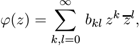 (1.40)
that converges for all z, and in which all coefficients bkl are nonnegative.
From this it follows that if p is a positive real number but not an even integer, then there exists a positive matrix A (of some size n depending on p) such that [[ |aij|p ]] is not positive.
Since ||A|| = || |A| || for all operators A, the triangle inequality may be expressed also as
If both A and B are normal, this can be improved. Using Corollary 1.3.8 we see that in this case
Then using Proposition 1.3.2 we obtain
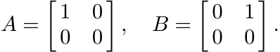
This inequality is stronger than (1.41). It is not true for all A and B, as may be seen from the example
The inequality (1.42) has an interesting application in the proof of Theorem 1.6.8 below.
1.6.7 Exercise
Let A and B be any two operators, and for a given positive integer m let ω = e2πi/m. Prove the identity
 (1.43)
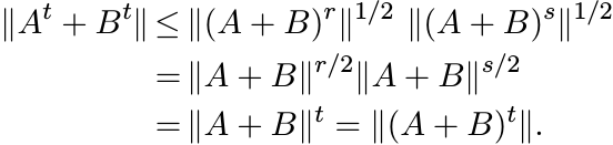
1.6.8 Theorem
Let A and B be positive operators. Then
Proof. Using the identity (1.43) we get
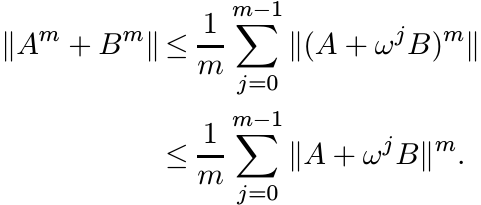 (1.45)
For each complex number z, the operator zB is normal. So from (1.42) we get
This shows that each of the summands in the sum on the right-hand side of (1.45) is bounded by ||A + B||m. Since A + B is positive, ||A + B||m = ||(A + B)m||. This proves the theorem. ■
The next theorem is more general.
1.6.9 Theorem
Let A and B be positive operators. Then
Proof. Let m be any positive integer and let Ωm be the set of all real numbers r in the interval [1, m] for which the inequality (1.46) is true. We will show that Ωm is a convex set. Since 1 and m belong to Ωm, this will prove the inequality (1.46).
Suppose r and s are two points in Ωm and let t = (r + s)/2. Then
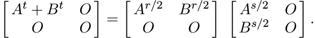
Hence
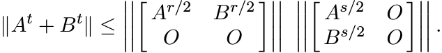
Since ||X|| = ||X∗X||1/2 = ||XX∗||1/2 for all X, this gives
We have assumed r and s are in Ωm. So, we have
This shows that t ∈ Ωm, and the inequality (1.46) is proved.
Let 0 < r ≤ 1. Then from (1.46) we have
Replacing A and B by Ar and Br, we obtain the inequality (1.47). ■
We have seen that AB+BA need not be positive when A and B are positive. Hence we do not always have A2 + B2 ≤ (A+ B)2. Theorem 1.6.8 shows that we do have the weaker assertion
1.6.10 Exercise
Use the example
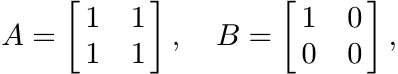
to see that the inequality
is not always true.
1.7 NOTES AND REFERENCES
Chapter 7 of the well known book Matrix Analysis by R. A. Horn and C. R. Johnson, Cambridge University Press, 1985, is an excellent source of information about the basic properties of positive definite matrices. See also Chapter 6 of F. Zhang, Matrix Theory: Basic Results and Techniques, Springer, 1999. The reader interested in numerical analysis should see Chapter 10 of N. J. Higham, Accuracy and Stability of Numerical Algorithms, Second Edition, SIAM 2002, and Chapter 5 of G. H. Golub and C. F. Van Loan, Matrix Computations, Third Edition, Johns Hopkins University Press, 1996.
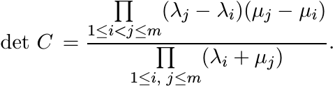
The matrix in (1.5) is a special case of the more general matrix C whose entries are
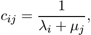
where (λ1, . . . , λm) and (µ1, . . . , µm) are any two real m-tuples. In 1841, Cauchy gave a formula for the determinant of this matrix:
From this it follows that the matrix in (1.5) is positive. The Hilbert matrix H with entries
is a special kind of Cauchy matrix. Hilbert showed that the infinite matrix H defines a bounded operator on the space l2 and ||H|| < 2π. The best value π for ||H|| was obtained by I. Schur, Bemerkungen zur Theorie der beschränkten Bilinearformen mit unendlich vielen Veränderlichen, J. Reine Angew. Math., 140 (1911). This is now called Hilbert’s inequality. See Chapter IX of G. H. Hardy, J. E. Littlewood, and G. Pólya, Inequalities, Second Edition, Cambridge University Press, 1952, for different proofs and interesting extensions. Chapter 28 of Higham’s book, cited earlier, describes the interest that the Hilbert and Cauchy matrices have for the numerical analyst.
Sylvester’s law of inertia is an important fact in the reduction of a real quadratic form to a sum of squares. While such a reduction may be achieved in many different ways, the law says that the number of positive and the number of negative squares are always the same in any such reduced representation. See Chapter X of F. Gantmacher, Matrix Theory, Chelsea, 1977. The law has special interest in the stability theory of differential equations where many problems depend on information on the location of the eigenvalues of matrices in the left half-plane. A discussion of these matters, and of the Lyapunov and Stein equations, may be found in P. Lancaster and M. Tismenetsky, The Theory of Matrices, Second Edition, Academic Press, 1985.
The Descartes rule of signs (in a slightly refined form) says that if all the roots of a polynomial f(x) are real, and the constant term is nonzero, then the number k1 of positive roots of the polynomial is equal to the number s1 of variations in sign in the sequence of its coefficients, and the number k2 of negative roots is equal to the number s2 of variations in sign in the sequence of coefficients of the polynomial f(−x). See, for example, A. Kurosh, Higher Algebra, Mir Publishers, 1972.
The symmetrized product (1.12), divided by 2, is also called the Jordan product. In Chapter 10 of P. Lax, Linear Algebra, John Wiley, 1997, the reader will find different (and somewhat longer) proofs of Propositions 1.2.6 and 1.2.9. Proposition 1.2.9 and Theorem 1.5.9 are a small part of Loewner’s theory of operator monotone functions. An exposition of the full theory is given in Chapter V of R. Bhatia, Matrix Analysis, Springer, 1997 (abbreviated to MA in our discussion).
The equation XAX = B in Exercise 1.2.13 is a very special kind of Riccati equation, the general form of such an equation being
Such equations arise in problems of control theory, and have been studied extensively. See, for example, P. Lancaster and L. Rodman, The Algebraic Riccati Equation, Oxford University Press, 1995.
Proposition 1.3.1 makes connection between an algebraic property–positivity, and
a metric property—contractivity. The technique of studying properties of a matrix
by embedding it in a larger matrix is known as “dilation theory” and has proved to
be of great value. An excellent demonstration of the power of such methods is given
in the two books by V. Paulsen, Completely Bounded Maps and Dilations, Longman,
1986 and Completely Bounded Maps and Operator Algebras, Cambridge University Press,
2002. Theorem 1.3.3 has been used to great effect by several authors. The idea behind
this 2 × 2 matrix calculation can be traced back to I. Schur, Über Potenzreihen die
im Innern des Einheitskreises beschränkt sind [I], J. Reine Angew. Math., 147 (1917)
205–232, where the determinantal identity of Exercise 1.5.6 occurs. Using the idea
in our first proof of Theorem 1.3.3 it is easy to deduce the following. If ![]() is a
Hermitian matrix and
is a
Hermitian matrix and ![]() is defined by (1.38), then we have the relation
is defined by (1.38), then we have the relation
between inertias. This fact was proved by E. Haynsworth, Determination of the inertia of a partitioned Hermitian matrix, Linear Algebra Appl., 1 (1968) 73–81. The term Schur complement was introduced by Haynsworth. The argument of Theorem 1.3.3 is a special case of this additivity of inertias.
The Schur complement is important in matrix calculations arising in several areas like statistics and electrical engineering. The recent book, The Schur Complement and Its Applications, edited by F. Zhang, Springer, 2005, contains several expository articles and an exhaustive bibliography that includes references to earlier expositions. The Schur complement is used in quantum mechanics as the decimation map or the Feshbach map. Here the Hamiltonian is a Hermitian matrix written in block form as
The block A corresponds to low energy states of the system without interaction. The decimated Hamiltonian is the matrix A−BD−1C. See W. G. Faris, Review of S. J. Gustafson and I. M. Sigal, Mathematical Concepts of Quantum Mechanics, SIAM Rev., 47 (2005) 379–380.
Perhaps the best-known theorem about the product A ◦ B is that it is positive when A and B are positive. This, together with other results like Theorem 1.4.1, was proved by I. Schur in his 1911 paper cited earlier.
For this reason, this product has been called the Schur product. Hadamard product is another name for it. The entertaining and informative article R. Horn, The Hadamard product, in Matrix Theory and Applications, C. R. Johnson, ed., American Math. Society, 1990, contains a wealth of historical and other detail. Chapter 5 of R. A. Horn and C. R. Johnson, Topics in Matrix Analysis, Cambridge University Press, 1991 is devoted to this topic. Many recent theorems, especially inequalities involving the Schur product, are summarised in the report T. Ando, Operator-Theoretic Methods for Matrix Inequalities, Sapporo, 1998.
Monotone and convex functions of self-adjoint operators have been studied extensively since the appearance of the pioneering paper by K. Löwner, Über monotone Matrixfunctionen, Math. Z., 38 (1934) 177–216. See Chapter V of MA for an introduction to this topic. The elegant and effective use of block matrices in this context is mainly due to T. Ando, Topics on Operator Inequalities, Hokkaido University, Sapporo, 1978, and Concavity of certain maps on positive definite matrices and applications to Hadamard products, Linear Algebra Appl. 26 (1979) 203–241.
The representation (1.40) for functions that preserve positivity (in the sense described) was established in C. S. Herz, Fonctions opérant sur les fonctions définies-positives, Ann. Inst. Fourier (Grenoble), 13 (1963) 161–180. A real variable version of this was noted earlier by I. J. Schoenberg.
Theorems 1.6.8 and 1.6.9 were proved in R. Bhatia and F. Kittaneh, Norm inequalities for positive operators, Lett. Math. Phys. 43 (1998) 225–231. A much more general result, conjectured in this paper and proved by T. Ando and X. Zhan, Norm inequalities related to operator monotone functions, Math. Ann., 315 (1999) 771–780, says that for every nonnegative operator monotone function f on [0, ∞) we have ||f(A + B)|| ≤ ||f(A) + f(B)|| for all positive matrices A and B. Likewise, if g is a nonnegative increasing function on [0, ∞) such that g(0) = 0, g(∞) = ∞, and the inverse function of g is operator monotone, then ||g(A) + g(B)|| ≤ ||g(A + B)||. This includes Theorem 1.6.9 as a special case. Further, these inequalities are valid for a large class of norms called unitarily invariant norms. (Operator monotone functions and unitarily invariant norms are defined in Section 2.7.) It may be of interest to mention here that, with the notations of this paragraph, we have also the inequalities ||f(A) − f(B)|| ≤ ||f(|A − B|)||, and ||g(|A − B|)|| ≤ ||g(A) − g(B)||. See Theorems X.1.3 and X.1.6 in MA. More results along these lines can be found in X. Zhan, Matrix Inequalities, Lecture Notes in Mathematics, Vol. 1790, Springer, 2002.
Many important and fundamental theorems of the rapidly developing subject of quantum information theory are phrased as inequalities for positive matrices (often block matrices). One popular book on this subject is M. A. Nielsen and I. L. Chuang, Quantum Computation and Quantum Information, Cambridge University Press, 2002.