
Chapter Three
Completely Positive Maps
For several reasons a special class of positive maps, called completely positive maps, is especially important. In Section 3.1 we study the basic properties of this class of maps. In Section 3.3 we derive some Schwarz type inequalities for this class; these are not always true for all positive maps. In Sections 3.4 and 3.5 we use general results on completely positive maps to study some important problems for matrix norms.
Let ![]() be the space of m× m block matrices [[Aij]] whose i, j entry is an element of
be the space of m× m block matrices [[Aij]] whose i, j entry is an element of
![]() . Each linear map
. Each linear map ![]() induces a linear map
induces a linear map ![]() defined as
defined as
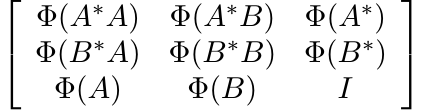
We say that Φ is m-positive if the map Φm is positive, and Φ is completely positive if it is m-positive for all m = 1, 2, . . .. Thus positive maps are 1-positive.
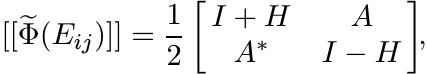
The map Φ(A) = Atr on ![]() is positive but not 2-positive. To see this consider the 2
× 2 matrices Eij whose i, j entry is one and the remaining entries are zero. Then
[[Eij]] is positive, but [[Φ(Eij)]] is not.
is positive but not 2-positive. To see this consider the 2
× 2 matrices Eij whose i, j entry is one and the remaining entries are zero. Then
[[Eij]] is positive, but [[Φ(Eij)]] is not.
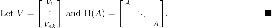
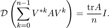
Let ![]() , the space of n × k matrices. Then the map Φ(A) = V ∗AV from
, the space of n × k matrices. Then the map Φ(A) = V ∗AV from ![]() into
into ![]() is completely
positive. To see this note that for each m
is completely
positive. To see this note that for each m
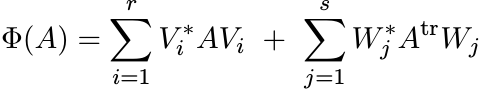
If ![]() , then
, then
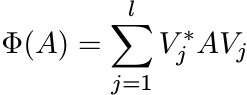 (3.2)
(3.2)is completely positive.
Let φ be any positive linear functional on ![]() . Then there exists a positive matrix
X such that φ(A) = tr AX for all A. If uj, 1 ≤ j ≤ n, constitute an orthonormal basis
for
. Then there exists a positive matrix
X such that φ(A) = tr AX for all A. If uj, 1 ≤ j ≤ n, constitute an orthonormal basis
for ![]() , then we have
, then we have
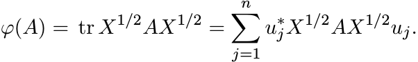
So, if we put vj = X1/2uj, we have
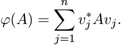
This shows that in the special case k = 1, every positive linear map ![]() can be represented
in the form (3.2) and thus is completely positive.
can be represented
in the form (3.2) and thus is completely positive.
3.1 SOME BASIC THEOREMS
Let us fix some notations. The standard basis for ![]() will be written as ej, 1 ≤ j ≤
n. The matrix
will be written as ej, 1 ≤ j ≤
n. The matrix ![]() will be written as Eij. This is the matrix with its i, j entry equal
to one and all other entries equal to zero. These matrices are called matrix units.
The family {Eij : 1 ≤ i, j ≤ n} spans
will be written as Eij. This is the matrix with its i, j entry equal
to one and all other entries equal to zero. These matrices are called matrix units.
The family {Eij : 1 ≤ i, j ≤ n} spans ![]() .
.
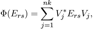
Our first theorem says all completely positive maps are of the form (3.2).
3.1.1 Theorem (Choi, Kraus)
Let ![]() be a completely positive linear map. Then there exist
be a completely positive linear map. Then there exist ![]() , such that
, such that
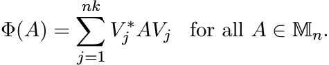 (3.3)
(3.3)
Proof. We will find Vj such that the relation (3.3) holds for all matrix units Ers
in ![]() . Since Φ is linear and the Ers span
. Since Φ is linear and the Ers span ![]() this is enough to prove the theorem.
this is enough to prove the theorem.
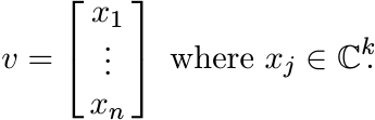
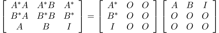
We need a simple identification involving outer products of block vectors. Let ![]() .
We think of v as a direct sum
.
We think of v as a direct sum ![]() , where
, where ![]() ; or as a column vector
; or as a column vector
Identify this with the k × n matrix
whose columns are the vectors xj. Then note that
So, if we think of vv∗ as an element of ![]() we have
we have
The matrix ![]() is a positive element of
is a positive element of ![]() . So, if
. So, if ![]() is an n-positive map, [[Φ(Ers)]] is
a positive element of
is an n-positive map, [[Φ(Ers)]] is
a positive element of ![]() .
.
By the spectral theorem, there exist vectors ![]() such that
such that
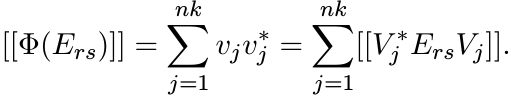
Thus for all 1 ≤ r, s ≤ n
as required. ■
Note that in the course of the proof we have shown that if a linear map ![]() is n-positive,
then it is completely positive. We have shown also that if Φn([[Ers]]) is positive,
then Φ is completely positive.
is n-positive,
then it is completely positive. We have shown also that if Φn([[Ers]]) is positive,
then Φ is completely positive.
The vectors vj occurring in the proof are not unique; and so the Vj in the representation are not unique. If we impose the condition that the family {vj} does not contain any zero vector and all vectors in it are mutually orthogonal, then the Vj in (3.3) are unique up to unitary conjugations. The proof of this statement is left as an exercise.
The map Φ is unital if and only if ![]() . Unital completely positive maps form a convex
set. We state, without proof, two facts about its extreme points. The extreme points
are those Φ for which the set {Vi∗Vj : 1 ≤ i, j ≤ nk} is linearly independent. For
such Φ, the number of terms in the representation (3.3) is at most k.
. Unital completely positive maps form a convex
set. We state, without proof, two facts about its extreme points. The extreme points
are those Φ for which the set {Vi∗Vj : 1 ≤ i, j ≤ nk} is linearly independent. For
such Φ, the number of terms in the representation (3.3) is at most k.
3.1.2 Theorem (The Stinespring Dilation Theorem)
Let ![]() be a completely positive map. Then there exist a representation
be a completely positive map. Then there exist a representation
and an operator
such that ||V ||2 = ||Φ(I)|| and
Proof. The equation (3.3) can be rewritten as
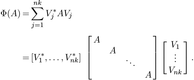
Note that if Φ is unital, then V ∗V = I. Hence V is an isometric embedding of ![]() in
in
![]() and V ∗ a projection. The representation
and V ∗ a projection. The representation ![]() is a direct sum of nk copies of A. This
number could be smaller in several cases. The representation with the minimal number
of copies is unique upto unitary conjugation.
is a direct sum of nk copies of A. This
number could be smaller in several cases. The representation with the minimal number
of copies is unique upto unitary conjugation.
3.1.3 Corollary
Let ![]() be completely positive. Then ||Φ|| = ||Φ(I)||. (This is true, more generally,
for all positive linear maps, as we saw in Chapter 2.)
be completely positive. Then ||Φ|| = ||Φ(I)||. (This is true, more generally,
for all positive linear maps, as we saw in Chapter 2.)
Next we consider linear maps whose domain is a linear subspace ![]() and whose range is
and whose range is
![]() . To each element Φ of
. To each element Φ of ![]() corresponds a unique element φ of
corresponds a unique element φ of ![]() . This correspondence is
described as follows. Let Sij, 1 ≤ i, j ≤ k be elements of
. This correspondence is
described as follows. Let Sij, 1 ≤ i, j ≤ k be elements of ![]() . Then
. Then
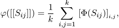 (3.5)
(3.5)where we use the notation [T]i,j for the i, j entry of a matrix T.
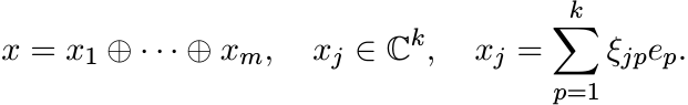
If ej, 1 ≤ j ≤ k is the standard basis for ![]() , and x is the vector in
, and x is the vector in ![]() given by
given by ![]() , then
(3.5) can be written as
, then
(3.5) can be written as
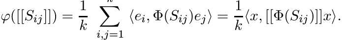 (3.6)
(3.6)
In the reverse direction, suppose φ is a linear functional on ![]() . Given an
. Given an ![]() let Φ(A)
be the element of
let Φ(A)
be the element of ![]() whose i, j entry is
whose i, j entry is
where Eij, 1 ≤ i, j ≤ k, are the matrix units in ![]() .
.
It is easy to see that this sets up a bijective correspondence between the spaces
![]() and
and ![]() . The factor 1/k in (3.5) ensures that Φ is unital if and only if φ is unital.
. The factor 1/k in (3.5) ensures that Φ is unital if and only if φ is unital.
3.1.4 Theorem
Let ![]() be an operator system in
be an operator system in ![]() , and let
, and let ![]() be a linear map. Then the following three
conditions are equivalent:
be a linear map. Then the following three
conditions are equivalent:
(i) Φ is completely positive.
(ii) Φ is k-positive.
(iii) The linear functional φ defined by (3.5) is positive.
Proof. Obviously (i) ![]() (ii). It follows from (3.6) that (ii)
(ii). It follows from (3.6) that (ii) ![]() (iii). The hard part
of the proof consists of establishing the implication (iii)
(iii). The hard part
of the proof consists of establishing the implication (iii) ![]() (i).
(i).
Since ![]() is an operator system in
is an operator system in ![]() is an operator system in
is an operator system in ![]() . By Krein’s extension
theorem (Theorem 2.6.6), the positive linear functional φ on
. By Krein’s extension
theorem (Theorem 2.6.6), the positive linear functional φ on ![]() has an extension
has an extension ![]() ,
a positive linear functional on
,
a positive linear functional on ![]() . To this
. To this ![]() corresponds an element
corresponds an element ![]() of
of ![]() defined via
(3.7). This
defined via
(3.7). This ![]() is an extension of Φ (since
is an extension of Φ (since ![]() is an extension of φ). If we show
is an extension of φ). If we show ![]() is
completely positive, it will follow that Φ is completely positive.
is
completely positive, it will follow that Φ is completely positive.
Let m be any positive integer. Every positive element of ![]() can be written as a sum
of matrices of the type
can be written as a sum
of matrices of the type ![]() where Aj, 1 ≤ j ≤ m are elements of
where Aj, 1 ≤ j ≤ m are elements of ![]() . To show that
. To show that ![]() is m-positive,
it suffices to show that
is m-positive,
it suffices to show that ![]() is positive. This is an mk × mk matrix. Let x be any vector
in
is positive. This is an mk × mk matrix. Let x be any vector
in ![]() . Write it as
. Write it as
Then
 (3.8)
(3.8)using (3.7). For 1 ≤ i ≤ m let Xi be the k × k matrix
Then ![]() . In other words
. In other words
So (3.8) can be written as
Since ![]() is positive, this expression is positive. That completes the proof. ■
is positive, this expression is positive. That completes the proof. ■
In the course of the proof we have also proved the following.
3.1.5 Theorem (Arveson’s Extension Theorem)
Let ![]() be an operator system in
be an operator system in ![]() and let
and let ![]() be a completely positive map. Then there
exists a completely positive map
be a completely positive map. Then there
exists a completely positive map ![]() that is an extension of Φ.
that is an extension of Φ.
Let us also record the following fact that we have proved.
3.1.6 Theorem
Let ![]() be a linear map. Let m = min(n, k). If Φ is m-positive, then it is completely
positive.
be a linear map. Let m = min(n, k). If Φ is m-positive, then it is completely
positive.
For l < m, there exists a map Φ that is l-positive but not (l + 1)-positive.
We have seen that completely positive maps have some desirable properties that positive
maps did not have: they can be extended from an operator system ![]() to the whole of
to the whole of
![]() , and they attain their norm at I for this reason (even when they have been defined
only on
, and they attain their norm at I for this reason (even when they have been defined
only on ![]() ). Also, there is a good characterization of completely positive maps given
by (3.3). No such simple representation seems possible for positive maps. For example,
one may ask whether every positive map
). Also, there is a good characterization of completely positive maps given
by (3.3). No such simple representation seems possible for positive maps. For example,
one may ask whether every positive map ![]() is of the form
is of the form
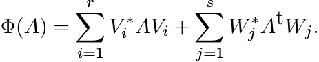
for some n × k matrices Vi, Wj. For n = k = 3, there exist positive maps Φ that can not be represented like this.
For these reasons the notion of complete positivity seems to be more useful than that of positivity.
We remark that many of the results of this section are true in the general setting of C∗-algebras. The proofs, naturally, are more intricate in the general setting.
In view of Theorem 3.1.6, one expects that if Φ is a positive linear map from a C∗-algebra a into a C∗-algebra b, and if either a or b is commutative, then Φ is completely positive. This is true.
3.2 EXERCISES
3.2.1
We have come across several positive linear maps in Chapter 2. Which of them are completely positive? What are (minimal) Stinespring dilations of these maps?
3.2.2
Every positive linear map Φ has a restricted 2-positive behaviour in the following sense:
[Hint: Use Proposition 2.7.3 and Proposition 2.7.5.]
3.2.3
Let Φ be a strictly positive linear map. Then the following three conditions are equivalent:
(i) Φ is 2-positive.
(ii) If A, B are positive matrices and X any matrix such that B ≥ X∗A−1X, then Φ(B) ≥ Φ(X)∗Φ(A)−1Φ(X).
(iii) For every matrix X and positive A we have Φ(X∗A−1X) ≥ Φ(X)∗ Φ(A)−1 Φ(X).
[Compare this with Exercise 2.7.4 and Proposition 2.7.5.]
3.2.4
Let ![]() be the map defined as Φ(A) = 2 (tr A) I − A. Then Φ is 2-positive but not 3-positive.
be the map defined as Φ(A) = 2 (tr A) I − A. Then Φ is 2-positive but not 3-positive.
3.2.5
Let A and B be Hermitian matrices and suppose A = Φ(B) for some doubly stochastic
map Φ on ![]() . Then there exists a completely positive doubly stochastic map Ψ such
that A = Ψ(B). (See Exercise 2.7.13.)
. Then there exists a completely positive doubly stochastic map Ψ such
that A = Ψ(B). (See Exercise 2.7.13.)
3.2.6
Let ![]() be the collection of all 2×2 matrices A with a11 = a22. This is an operator
system in
be the collection of all 2×2 matrices A with a11 = a22. This is an operator
system in ![]() . Show that the map Φ(A) = Atr is completely positive on
. Show that the map Φ(A) = Atr is completely positive on ![]() . What is its
completely positive extension on
. What is its
completely positive extension on ![]() ?
?
3.2.7
Suppose [[Aij]] is a positive element of ![]() . Then each of the m × m matrices
. Then each of the m × m matrices ![]() , and
, and
![]() is positive.
is positive.
3.3 SCHWARZ INEQUALITIES
In this section we prove some operator versions of the Schwarz inequality. Some of them are extensions of the basic inequalities for positive linear maps proved in Chapter 2.
Let µ be a probability measure on a space X and consider the Hilbert space L2(X,
µ). Let Ef = ![]() fdµ be the expectation of a function f. The covariance between two
functions f and g in L2(X, µ) is the quantity
fdµ be the expectation of a function f. The covariance between two
functions f and g in L2(X, µ) is the quantity
The variance of f is defined as
(We have come across this earlier in (2.23) where we restricted ourselves to real-valued functions.) The expression (3.9) is plainly an inner product in L2(X, µ) and the usual Schwarz inequality tells us
This is an important, much used, inequality in statistics.
As before, replace L2(X, µ) by ![]() and the expectation E by a positive unital linear
map Φ on
and the expectation E by a positive unital linear
map Φ on ![]() . The covariance between two elements A and B of
. The covariance between two elements A and B of ![]() (with respect to a given
Φ) is defined as
(with respect to a given
Φ) is defined as
and variance of A as
Kadison’s inequality (2.5) says that if A is Hermitian, then var(A) ≥ O. Choi’s generalization
(2.6) says that this is true also when A is normal. However, with no restriction
on A this is not always true. (Let Φ(A) = Atr, and let ![]() .)
.)
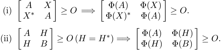
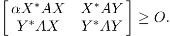
If Φ is unital and 2-positive, then by Exercise 3.2.3(iii) we have
for all A. This says that var(A) ≥ O for all A if Φ is 2-positive and unital. The inequality (3.14) says that
The inequality |Φ(A)| ≤ Φ(|A|) is not always true even when Φ is completely positive.
Let Φ be the pinching map on ![]() . If A =
. If A = ![]() , then
, then ![]() and
and ![]() .
.
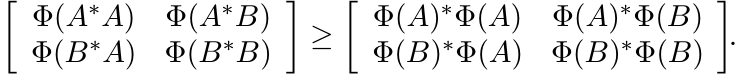
An analogue of the variance-covariance inequality (3.11) is given by the following theorem.
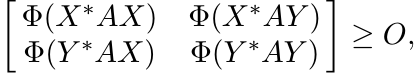
3.3.1 Theorem
Let Φ be a unital completely positive linear map on ![]() . Then for all A, B
. Then for all A, B
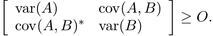 (3.16)
Proof. Let V be an isometry of the space ![]() into any
into any ![]() . Then V ∗V = I and V V ∗ ≤ I.
From the latter condition it follows that
. Then V ∗V = I and V V ∗ ≤ I.
From the latter condition it follows that

This is the same as saying
This inequality is preserved when we multiply both sides by the matrix ![]() on the left
and by
on the left
and by ![]() on the right. Thus
on the right. Thus

This is the inequality (3.16) for the special map Φ(T) = V ∗TV. The general case follows from this using Theorem 3.1.2. ■
3.3.2 Remark
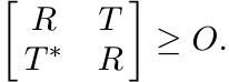
It is natural to wonder whether complete positivity of Φ is necessary for the inequality (3.16). It turns out that 2-positivity is not enough but 3-positivity is. Indeed, if Φ is 3-positive and unital, then from the positivity of the matrix
it follows that the matrix
is positive. Hence by Theorem 1.3.3 (see Exercise 1.3.5)

In other words,
 (3.17)
This is the same inequality as (3.16).
To see that this inequality is not always true for 2-positive maps, choose the map
Φ on ![]() as in Exercise 3.2.4. Let A = E13, and B = E12, where Eij stands for the matrix
whose i, j entry is one and all other entries are zero. A calculation shows that
the inequality (3.17) is not true in this case.
as in Exercise 3.2.4. Let A = E13, and B = E12, where Eij stands for the matrix
whose i, j entry is one and all other entries are zero. A calculation shows that
the inequality (3.17) is not true in this case.
3.3.3 Remark
If Φ is 2-positive, then for all A and B we have
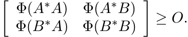 (3.18)
The inequality (3.17) is a considerable strengthening of this under the additional assumption that Φ is 3-positive and unital. The inequality (3.18) is equivalent to
(for 2-positive linear maps Φ). This is an operator version of the Schwarz inequality.
3.4 POSITIVE COMPLETIONS AND SCHUR PRODUCTS
A completion problem gives us a matrix some of whose entries are not specified, and asks us to fill in these entries in such a way that the matrix so obtained (called a completion) has a given property.
For example, we are given a 2 × 2 matrix ![]() with only three of its entries and are
asked to choose the unknown (2,2) entry in such a way that the norm of the completed
matrix is minimal among all completions. Such a completion is obtained by choosing
the (2,2) entry to be −1. This is an example of a minimal norm completion problem.
with only three of its entries and are
asked to choose the unknown (2,2) entry in such a way that the norm of the completed
matrix is minimal among all completions. Such a completion is obtained by choosing
the (2,2) entry to be −1. This is an example of a minimal norm completion problem.
A positive completion problem asks us to fill in the unspecified entries in such
a way that the completed matrix is positive. Sometimes further restrictions may be
placed on the completion. For example the incomplete matrix ![]() has several positive
completions: we may choose any two diagonal entries a, b such that a, b are positive
and ab ≥ 1. Among these the choice that minimises the norm of the completion is a
= b = 1.
has several positive
completions: we may choose any two diagonal entries a, b such that a, b are positive
and ab ≥ 1. Among these the choice that minimises the norm of the completion is a
= b = 1.
To facilitate further discussion, let us introduce some definitions.
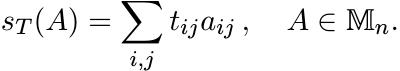
A subset J of {1, 2, . . . , n} × {1, 2, . . . , n} is called a pattern. A pattern J is called symmetric if
(i, i) ∈ J for 1 ≤ i ≤ n, and
(i, j) ∈ J if and only if (j, i) ∈ J.
We say T is a partially defined matrix with pattern J if the entries tij are specified
for all (i, j) ∈ J. We call such a_ T symmetric if J is symmetric, tii is real for
all 1 ≤ i ≤ n, and ![]() for (i, j) ∈ J.
for (i, j) ∈ J.
Given a pattern J, let
This is a subspace of ![]() , and it is an operator system if the pattern J is symmetric.
, and it is an operator system if the pattern J is symmetric.
For ![]() , we use the notation ST for the linear operator
, we use the notation ST for the linear operator
and sT for the linear functional
3.4.1 Theorem
Let T be a partially defined symmetric matrix with pattern J. Then the following three conditions are equivalent:
(i) T has a positive completion.
(ii)
The linear map ![]() is positive.
is positive.
(iii)
The linear functional sT on ![]() is positive.
is positive.
Proof. If T has a positive completion ![]() , then by Schur’s theorem
, then by Schur’s theorem ![]() is a positive map
on
is a positive map
on ![]() . For
. For ![]() . So, ST is positive on
. So, ST is positive on ![]() . This proves the implication (i)
. This proves the implication (i) ![]() (ii). The implication
(ii)
(ii). The implication
(ii) ![]() (iii) is obvious. (The sum of all entries of a positive matrix is a nonnegative
number.)
(iii) is obvious. (The sum of all entries of a positive matrix is a nonnegative
number.)
(iii) ![]() (i): Suppose sT is positive. By Krein’s extension theorem there exists a positive
linear functional s on
(i): Suppose sT is positive. By Krein’s extension theorem there exists a positive
linear functional s on ![]() that extends sT. Let
that extends sT. Let ![]() . Then the matrix
. Then the matrix ![]() is a completion of
T. We have for every vector x
is a completion of
T. We have for every vector x
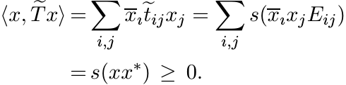
Thus ![]() is positive. ■
is positive. ■
For T ∈ ![]() let T# be the element of
let T# be the element of ![]() defined as
defined as ![]() . We have seen that T is a contraction
if and only if T# is positive.
. We have seen that T is a contraction
if and only if T# is positive.
3.4.2 Proposition
Let ![]() be the operator system in
be the operator system in ![]() defined as
defined as
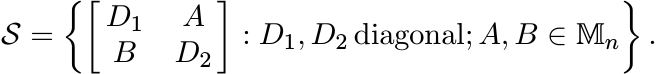
Then for any T ∈ ![]() , the Schur multiplier ST is contractive on
, the Schur multiplier ST is contractive on ![]() if and only if ST#
is a positive linear map on the operator system
if and only if ST#
is a positive linear map on the operator system ![]() .
.
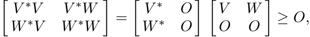
Proof. Suppose ST# is positive on S. Then
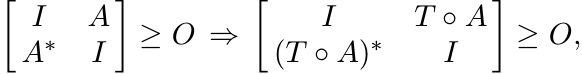
i.e., ||A|| ≤ 1 ![]() ||T ◦ A|| ≤ 1. In other words ST is contractive on
||T ◦ A|| ≤ 1. In other words ST is contractive on ![]() .
.
To prove the converse, assume D1, D2 > O, and note that
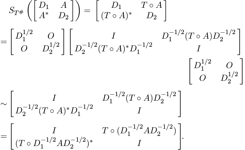
If ST is contractive on ![]() , then
, then
i.e.,

We have seen above that the last matrix is congruent to
![]() . This shows that ST# is positive on
. This shows that ST# is positive on ![]() . ■
. ■
We can prove now the main theorem of this section.
3.4.3 Theorem (Haagerup’s Theorem)
Let T ∈ ![]() . Then the following four conditions are equivalent:
. Then the following four conditions are equivalent:
(i) ST is contractive; i.e., ||T ◦ A|| ≤ ||A|| for all A.
(ii) There exist vectors vj, wj, 1 ≤ j ≤ n, all with their norms ≤ 1, such that tij = vı∗wj.
(iii)
There exist positive matrices R1, R2 with diag R1 ≤ I, diag R2 ≤ I and such that
![]() is positive.
is positive.
(iv) T can be factored as T = V ∗W with ||V ||c ≤ 1, ||W ||c ≤ 1. (The symbol ||Y ||c stands for the maximum of the Euclidean norms of the columns of Y.)
Proof. Let ST be contractive. Then, by Proposition 3.4.2, ST# is a positive operator
on the operator system ![]() . By Theorem 3.4.1, T# has a positive completion. (Think of
the off-diagonal entries of the two diagonal blocks as unspecified.) Call this completion
P. It has a Cholesky factoring P = Δ∗Δ where Δ is an upper triangular 2n × 2n matrix.
Write
. By Theorem 3.4.1, T# has a positive completion. (Think of
the off-diagonal entries of the two diagonal blocks as unspecified.) Call this completion
P. It has a Cholesky factoring P = Δ∗Δ where Δ is an upper triangular 2n × 2n matrix.
Write ![]() . Then
. Then
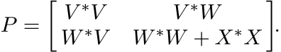
Let vj, wj, 1 ≤ j ≤ n be the columns of V, W, respectively. Since P is a completion
of T#, we have T = V ∗W; i.e., ![]() . Since diag(V ∗V ) = I, we have ||vj|| = 1. Since
diag(W∗W + X∗X) = I, we have ||wj|| ≤ 1. This proves the implication (i)
. Since diag(V ∗V ) = I, we have ||vj|| = 1. Since
diag(W∗W + X∗X) = I, we have ||wj|| ≤ 1. This proves the implication (i) ![]() (ii).
(ii).
The condition (ii) can be expressed by saying T = V ∗W, where diag(V ∗V ) ≤ I and diag(W∗W) ≤ I. Since
this shows that the statement (ii) implies (iii). Clearly (iv) is another way of stating (ii).
To complete the proof we show that (iii) ![]() (i). Let A ∈
(i). Let A ∈ ![]() , ||A|| ≤ 1. This implies
, ||A|| ≤ 1. This implies
![]() . Then the condition (iii) leads to the inequality
. Then the condition (iii) leads to the inequality
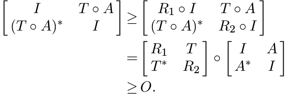
But this implies ||T ◦ A|| ≤ 1. In other words ST is contractive. ■
3.4.4 Corollary
For every T in ![]() , we have ||ST || = min {||V ||c ||W||c : T = V *W} .
, we have ||ST || = min {||V ||c ||W||c : T = V *W} .
3.5 THE NUMERICAL RADIUS
The numerical range of an operator A is the set of complex numbers
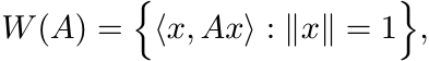
and the numerical radius is the number
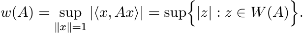
It is known that the set W(A) is convex, and w(·) defines a norm. We have
Some properties of w are summarised below. It is not difficult to prove them.
(i) w(UAU∗) = w(A) for all A, and unitary U.
(ii) If A is diagonal, then w(A) = max |aii|.
(iii) More generally,
(iv) w(A) = ||A|| if (but not only if) A is normal.
(v) w is not submultiplicative: the inequality w(AB) ≤ w(A)w(B) is not always true for 2 × 2 matrices.
(vi) Even the weaker inequality w(AB) ≤ ||A||w(B) is not always true for 2 × 2 matrices.
(vii)
The inequality ![]() is not always true for 2 × 2 matrices A, B.
is not always true for 2 × 2 matrices A, B.
(viii)
However, we do have ![]() for square matrices A, B of any size.
for square matrices A, B of any size.
(Proof: It is enough to prove this when ||A|| = 1. Then A = ![]() where U, V are unitary.
So it is enough to prove that
where U, V are unitary.
So it is enough to prove that ![]() if U is unitary. Choose an orthonormal basis in which
U is diagonal, and use (iii).)
if U is unitary. Choose an orthonormal basis in which
U is diagonal, and use (iii).)
(ix)
If w(A) ≤ 1, then I ± ReA ≥ O.
![]()
(x) The inequality w(AB) ≤ w(A)w(B) may not hold even when A, B commute. Let
Then w(A) < 1, w(A2) = w(A3) = 1/2. So w(A3) > w(A)w(A2) in this case.
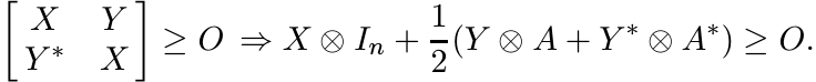
Proposition 1.3.1 characterizes operators A with ||A|| ≤ 1 in terms of positivity of certain 2 × 2 block matrices. A similar theorem for operators A with w(A) ≤ 1 is given below.
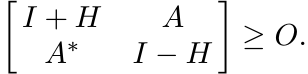
3.5.1 Theorem (Ando)
Let A ∈ ![]() . Then w(A) ≤ 1 if and only if there exists a Hermitian matrix H such that
. Then w(A) ≤ 1 if and only if there exists a Hermitian matrix H such that
![]() is positive.
is positive.
Proof. If ![]() , then there exists an operator K with ||K|| ≤ 1 such that A = (I + H)1/2K(I
− H)1/2. So, for every vector x
, then there exists an operator K with ||K|| ≤ 1 such that A = (I + H)1/2K(I
− H)1/2. So, for every vector x
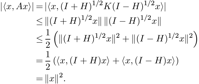
This shows that w(A) ≤ 1.
The proof of the other half of the theorem is longer. Let A be an operator with w(A)
≤ 1. Let ![]() be the collection of 2 × 2 matrices
be the collection of 2 × 2 matrices ![]() where x, y, z are complex numbers.
Then
where x, y, z are complex numbers.
Then ![]() is an operator system. Let
is an operator system. Let ![]() be the unital linear map defined as
be the unital linear map defined as
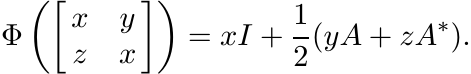
It follows from property (ix) listed at the beginning of the section that Φ is positive.
We claim it is completely positive. Let m be any positive integer. We want to show
that if the m× m block matrix with the 2 × 2 block ![]() as its i, j entry is positive,
then the m × m block matrix with the n×n block xijI + 2 1 (yijA+zijA∗) as its i,
j entry is also positive. Applying permutation similarity the first matrix can be
converted to a matrix of the form
as its i, j entry is positive,
then the m × m block matrix with the n×n block xijI + 2 1 (yijA+zijA∗) as its i,
j entry is also positive. Applying permutation similarity the first matrix can be
converted to a matrix of the form ![]() where X, Y, Z are m× m matrices. If this is positive,
then we have Z = Y ∗, and our claim is that
where X, Y, Z are m× m matrices. If this is positive,
then we have Z = Y ∗, and our claim is that
We can apply a congruence, and replace the matrices X by I and Y by X−1/2Y X−1/2, respectively. Thus we need to show that

The hypothesis here is (equivalent to) ||Y || ≤ 1. By property (viii) this implies
![]() . So the conclusion follows from property (ix).
. So the conclusion follows from property (ix).
We have shown that Φ is completely positive on ![]() . By Arveson’s theorem Φ can be extended
to a completely positive map
. By Arveson’s theorem Φ can be extended
to a completely positive map ![]()
![]() .
.
Let Eij, 1 ≤ i, j ≤ 2 be the matrix units in ![]() . Then the matrix
. Then the matrix ![]() is positive. Thus,
in particular,
is positive. Thus,
in particular, ![]() and
and ![]() are positive, and their sum is I since
are positive, and their sum is I since ![]() is unital.
is unital.
Put ![]() . Then H is Hermitian, and
. Then H is Hermitian, and
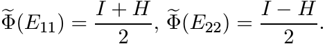
Since ![]() is an extension of Φ, we have
is an extension of Φ, we have
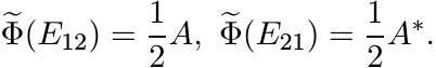
Thus
and this matrix is positive. ■
3.5.2 Corollary
For every A and k = 1, 2, . . .
Proof. It is enough to show that if w(A) ≤ 1, then w(Ak) ≤ 1. Let w(A) ≤ 1. By Ando’s theorem, there exists a Hermitian matrix H such that
Hence, there exists a contraction K such that
Then
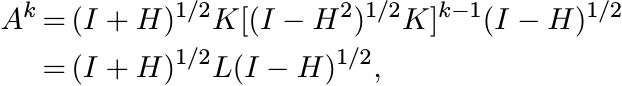
where L = K[(I − H2)1/2K]k−1 is a contraction. But this implies that
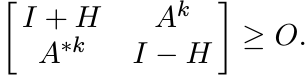
So, by Ando’s Theorem w(Ak) ≤ 1. ■
The inequality (3.20) is called the power inequality for the numerical radius.
Ando and Okubo have proved an analogue of Haagerup’s theorem for the norm of the Schur product with respect to the numerical radius. We state it without proof.
3.5.3 Theorem (Ando-Okubo)
Let T be any matrix. Then the following statements are equivalent:
(i) w(T ◦ A) ≤ 1 whenever w(A) ≤ 1.
(ii) There exists a positive matrix R with diagR ≤ I such that
3.6 SUPPLEMENTARY RESULTS AND EXERCISES
The Schwarz inequality, in its various forms, is the most important inequality in analysis. The first few remarks in this section supplement the discussion in Section 3.3.
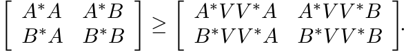
Let A be an n × k matrix and B an n × l matrix of rank l. The matrix
is positive. This is equivalent to the assertion
This is a matrix version of the Schwarz inequality. It can be proved in another way as follows. The matrix B(B∗B)−1B∗ is idempotent and Hermitian. Hence I ≥ B(B∗B)−1B∗ and (3.21) follows immediately. The inequality (3.19) is an extension of (3.21).
Let A be a positive operator and let x, y be any two vectors. From the Schwarz inequality we get
An operator version of this in the spirit of (3.19) can be obtained as follows. For any two operators X and Y we have

So, if Φ is a 2-positive linear map, then
or, equivalently,
This is an operator version of (3.22).
There is a considerable strengthening of the inequality (3.22) in the special case
when x is orthogonal to y. This says that if A is a positive operator with mI ≤ A
≤ MI, and ![]() , then
, then
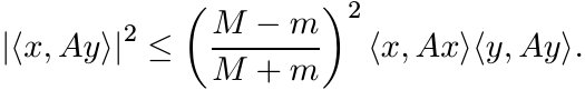 (3.24)
This is called Wielandt’s inequality. The following theorem gives an operator version.
3.6.1 Theorem
Let A be a positive element of ![]() with mI ≤ A ≤ MI. Let X, Y be two mutually orthogonal
projection operators in
with mI ≤ A ≤ MI. Let X, Y be two mutually orthogonal
projection operators in ![]() . Then for every 2-positive linear map Φ on
. Then for every 2-positive linear map Φ on ![]() we have
we have
 (3.25)
Proof. First assume that ![]() . With respect to this decomposition, let A have the block
form
. With respect to this decomposition, let A have the block
form
By Exercise 1.5.7
Apply Proposition 2.7.8 with Φ as the pinching map. This shows
Taking inverses changes the direction of this inequality, and then rearranging terms we get
This is the inequality (3.25) in the special case when Φ is the identity map. A minor
argument shows that the assumption ![]() can be dropped.
can be dropped.
Let α = (M − m)/(M + m). The inequality we have just proved is equivalent to the statement
This implies that the inequality (3.25) holds for every 2-positive linear map Φ. ■
We say that a complex function f on ![]() is in the Lieb class
is in the Lieb class ![]() if f(A) ≥ 0 whenever A
≥ O, and |f(X)|2 ≤ f(A)f(B) whenever
if f(A) ≥ 0 whenever A
≥ O, and |f(X)|2 ≤ f(A)f(B) whenever ![]() . Several examples of such functions are given
in MA (pages 268–270). We have come across several interesting 2 × 2 block matrices
that are positive. Many Schwarz type inequalities for functions in the class L can
be obtained from these block matrices.
. Several examples of such functions are given
in MA (pages 268–270). We have come across several interesting 2 × 2 block matrices
that are positive. Many Schwarz type inequalities for functions in the class L can
be obtained from these block matrices.
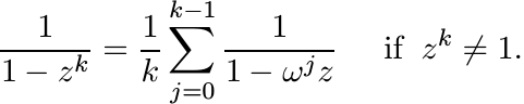
The next few results concern maps associated with pinchings and their norms.
Let ![]() be the diagonal part of a matrix:
be the diagonal part of a matrix:
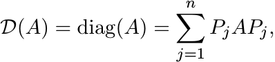 (3.26)
where ![]() is the orthogonal projection onto the one-dimensional space spanned by the
vector ej. This is a special case of the pinching operation C introduced in Example
2.2.1 (vii). Since
is the orthogonal projection onto the one-dimensional space spanned by the
vector ej. This is a special case of the pinching operation C introduced in Example
2.2.1 (vii). Since ![]() and Pj ≥ O, we think of the sum (3.26) as a noncommutative convex
combination. There is another interesting way of expressing for
and Pj ≥ O, we think of the sum (3.26) as a noncommutative convex
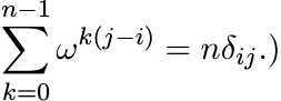
combination. There is another interesting way of expressing for ![]() . Let ω = e2πi/n
and let U be the diagonal unitary matrix
. Let ω = e2πi/n
and let U be the diagonal unitary matrix
Then
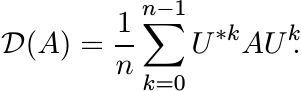 (3.28)
(The sum on the right-hand side is the Schur product of A by a matrix whose i, j entry is
This idea can be generalized.
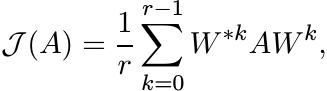
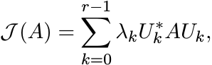
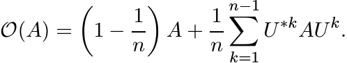
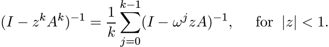
3.6.2 Exercise
Partition n × n matrices into an r × r block form in which the diagonal blocks are square matrices of dimension d1, . . . , dr. Let C be the pinching operation sending the block matrix A = [[Aij]] to the block diagonal matrix C(A) = diag(A11, . . . , Arr). Let ω = e2πi/r and let V be the diagonal unitary matrix
where Ij is the identity matrix of size dj. Show that
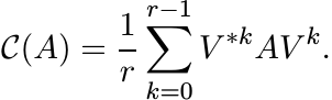 (3.29)
3.6.3 Exercise
Let J be a pattern and let ![]() be the map on
be the map on ![]() induced by J as follows. The i, j entry
of
induced by J as follows. The i, j entry
of ![]() is aij for all (i, j) ∈ J and is zero otherwise. Suppose J is an equivalence
relation on {1, 2, . . . , n} and has r equivalence classes. Show that
is aij for all (i, j) ∈ J and is zero otherwise. Suppose J is an equivalence
relation on {1, 2, . . . , n} and has r equivalence classes. Show that
 (3.30)
where W is a diagonal unitary matrix. Conversely, show that if ![]() can be represented
as
can be represented
as
 (3.31)
where Uj are unitary matrices and λj are positive numbers with ![]() , then J is an equivalence
relation with r equivalence classes. It is not possible to represent
, then J is an equivalence
relation with r equivalence classes. It is not possible to represent ![]() as a convex
combination of unitary transforms as in (3.31) with fewer than r terms.
as a convex
combination of unitary transforms as in (3.31) with fewer than r terms.
3.6.4 Exercise
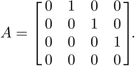
Let V be the permutation matrix
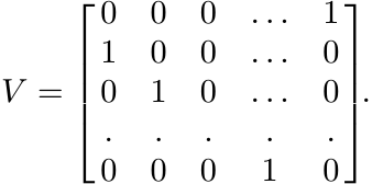 (3.32)
Show that
 (3.33)
Find n2 unitary matrices Wj such that
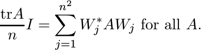 (3.34)
This gives a representation of the linear map ![]() from
from ![]() into scalar matrices.
into scalar matrices.
It is of some interest to consider what is left of a matrix after the diagonal part is removed. Let
be the off-diagonal part of A. Using (3.28) we can write
From this we get
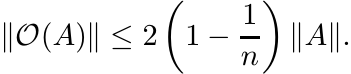 (3.36)
This inequality is sharp. To see this choose ![]() , where E is the matrix all of whose
entries are equal to one.
, where E is the matrix all of whose
entries are equal to one.
3.6.5 Exercise
Let B = E − I. We have just seen that the Schur multiplier norm
 (3.37)
Find an alternate proof of this using Theorem 3.4.3.
3.6.6 Exercise
Use Exercise 3.6.3 to show that
This inequality can be improved:
(i)
Every matrix is unitarily similar to one with constant diagonal entries. [Prove
this by induction, with the observation that ![]() for some unit vector x.]
for some unit vector x.]
(ii)
Thus, in some orthonormal basis, removing ![]() has the same effect as removing
has the same effect as removing ![]() from
A. Thus
from
A. Thus
 (3.38)
and this inequality is sharp.
3.6.7 Exercise
The Schur multiplier norm is multiplicative over tensor products; i.e.,
3.6.8 Exercise
Let ![]() . Show, using Theorem 3.4.3 and otherwise, that
. Show, using Theorem 3.4.3 and otherwise, that
Let Δn be the triangular truncation operator taking every n×n matrix to its upper
triangular part. Then we have ![]() . Try to find ||Δ3||.
. Try to find ||Δ3||.
3.6.9 Exercise
Fill in the details in the following proof of the power inequality (3.20).
(i) If a is a complex number, then |a| ≤ 1 if and only if Re(1−za) ≥ 0 for all z with |z| < 1.
(ii) w(A) ≤ 1 if and only if Re(I − zA) ≥ O for |z| < 1.
(iii) w(A) ≤ 1 if and only if Re((I − zA)−1) ≥ O for |z| < 1.
(iv) Let ω = e2πi/k. Prove the identity
(v) If w(A) ≤ 1, then
(vi) Assume w(A) ≤ 1. Use (v) and (iii) to conclude that w(Ak) ≤ 1.
By Exercise 3.2.7, if [[Aij]] is a positive element of ![]() , then the m × m matrices
[[ tr Aij ]] and
, then the m × m matrices
[[ tr Aij ]] and ![]() are positive. Matricial curiosity should make us wonder whether
this remains true when tr is replaced by other matrix functions like det, and the
norm || · ||2 is replaced by the norm || · ||.
are positive. Matricial curiosity should make us wonder whether
this remains true when tr is replaced by other matrix functions like det, and the
norm || · ||2 is replaced by the norm || · ||.
For the sake of economy, in the following discussion we use (temporarily) the terms
positive, m-positive, and completely positive to encompass nonlinear maps as well.
Thus we say a map ![]() is positive if Φ(A) ≥ O whenever A ≥ O, and completely positive
if [[Φ(Aij)]] is positive whenever a block matrix [[Aij]] is positive. For example,
det(A) is a positive (nonlinear) function, and we have observed that
is positive if Φ(A) ≥ O whenever A ≥ O, and completely positive
if [[Φ(Aij)]] is positive whenever a block matrix [[Aij]] is positive. For example,
det(A) is a positive (nonlinear) function, and we have observed that ![]() is a completely
positive (nonlinear) function. In Chapter 1 we noted that a function
is a completely
positive (nonlinear) function. In Chapter 1 we noted that a function ![]() is completely
positive if and only if it can be expressed in the form (1.40).
is completely
positive if and only if it can be expressed in the form (1.40).
3.6.10 Proposition
Let φ(A) = ||A||2. Then φ is 2-positive but not 3-positive.
Proof. The 2-positivity is an easy consequence of Proposition 1.3.2. The failure
of φ to be 3-positive is illustrated by the following example in ![]() . Let
. Let
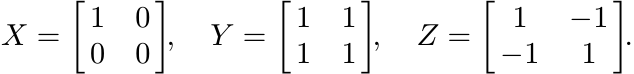
Since X, Y and Z are positive, so is the matrix
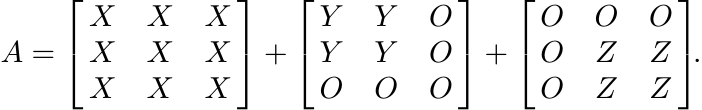
If we write A as [[Aij]] where Aij, 1 ≤ i, j ≤ 3 are 2 × 2 matrices, and replace each Aij by ||Aij||2 we obtain the matrix
This matrix is not positive as its determinant is negative. ■
3.6.11 Exercise
Let ![]() be the map defined as Φ(X) = |X|2 = X∗X. Use the example in Exercise 1.6.6 to
show that Φ is not two-positive.
be the map defined as Φ(X) = |X|2 = X∗X. Use the example in Exercise 1.6.6 to
show that Φ is not two-positive.
3.6.12 Exercise
Let ![]() be the k-fold tensor power of A. Let A = [[Aij]] be an element of
be the k-fold tensor power of A. Let A = [[Aij]] be an element of ![]() . Then
. Then ![]() is
a matrix of size (mn)k whereas
is
a matrix of size (mn)k whereas ![]() is a matrix of size mnk. Show that the latter is
a principal submatrix of the former. Use this observation to conclude that
is a matrix of size mnk. Show that the latter is
a principal submatrix of the former. Use this observation to conclude that ![]() is a
completely positive map from
is a
completely positive map from ![]() to
to ![]() .
.
3.6.13 Exercise
For 1 ≤ k ≤ n let ∧kA be the kth antisymmetric tensor power of an n × n matrix A.
Show that ∧k is a completely positive map from ![]() into
into ![]() . If
. If
is the characteristic polynomial of A, then ck(A) = tr ∧kA. Hence each ck is a completely positive functional. In particular, det is completely positive.
Similar considerations apply to other “symmetry classes” of tensors and the associated “Schur functions.” Thus, for example, the permanent function is completely positive.
3.6.14 Exercise
Let ![]() be any 4-positive map. Let X, Y, Z be positive elements of
be any 4-positive map. Let X, Y, Z be positive elements of ![]() and let
and let
Then A = [[Aij]] is positive. Let X = [I, −I, I, −I]. Consider the product X[[Φ(Aij)]]X∗ and conclude that
Inequalities of the form (3.39) occur in other contexts. For example, if P, Q and R are (rectangular) matrices and the product P QR is defined, then the Frobenius inequality is the relation between ranks:
The inequality (4.49) in Chapter 4 is another one with a similar structure.
3.7 NOTES AND REFERENCES
The theory of completely positive maps has been developed by operator algebraists and mathematical physicists over the last four decades.
The two major results of Section 3.1, the theorems of Stinespring and Arveson, hold in much more generality. We have given their baby versions by staying in finite dimensions.
Stinespring’s theorem was proved in W. F. Stinespring, Positive functions on C∗-algebras, Proc. Amer. Math. Soc., 6 (1955) 211–216. To put it in context, it is helpful to recall an earlier theorem due to M. A. Naimark.
Let ![]() be a compact Hausdorff space with its Borel σ-algebra
be a compact Hausdorff space with its Borel σ-algebra ![]() , and let
, and let ![]() ) be the collection
of orthogonal projections in a Hilbert space
) be the collection
of orthogonal projections in a Hilbert space ![]() . A projection-valued measure is a map
. A projection-valued measure is a map
![]() from
from ![]() into
into ![]() that is countably additive: if {Si} is a countable collection of disjoint
sets, then
that is countably additive: if {Si} is a countable collection of disjoint
sets, then
for all x and y in ![]() . The spectral theorem says that if A is a bounded self-adjoint
operator on
. The spectral theorem says that if A is a bounded self-adjoint
operator on ![]() , then there exists a projection-valued measure on [−||A||, ||A||] taking
values in
, then there exists a projection-valued measure on [−||A||, ||A||] taking
values in ![]() , and with respect to this measure A can be written as the integral
, and with respect to this measure A can be written as the integral ![]() .
.
Instead of projection-valued measures we may consider an operator-valued measure.
This assigns to each set S an element E(S) of ![]() , the map is countably additive, and
sup {||E(S)|| : S ∈
, the map is countably additive, and
sup {||E(S)|| : S ∈ ![]() } < ∞. Such a measure gives rise to a complex measure
} < ∞. Such a measure gives rise to a complex measure
for each pair x, y in ![]() . This in turn gives a bounded linear map Φ from the space
C(X) into
. This in turn gives a bounded linear map Φ from the space
C(X) into ![]() via
via
 (3.41)
This process can be reversed. Given a bounded linear map Φ : ![]() we can construct complex
measures µx,y via (3.40) and then an operator-valued measure E via (3.39). If E(S)
is a positive operator for all S, we say the measure E is positive.
we can construct complex
measures µx,y via (3.40) and then an operator-valued measure E via (3.39). If E(S)
is a positive operator for all S, we say the measure E is positive.
Naimark’s theorem says that every positive operator-valued measure can be dilated
to a projection-valued measure. More precisely, if E is a positive ![]() -valued measure
on
-valued measure
on ![]() , then there exist a Hilbert space
, then there exist a Hilbert space ![]() , a bounded linear map
, a bounded linear map ![]() , and a
, and a ![]() - valued measure
P such that
- valued measure
P such that
The point of the theorem is that by dilating to the space ![]() we have replaced the operator-valued
measure E by the projection-valued measure P which is nicer in two senses: it is
more familiar because of its connections with the spectral theorem and the associated
map Φ is now a ∗-homomorphism of C(X).
we have replaced the operator-valued
measure E by the projection-valued measure P which is nicer in two senses: it is
more familiar because of its connections with the spectral theorem and the associated
map Φ is now a ∗-homomorphism of C(X).
The Stinespring theorem is a generalization of Naimark’s theorem in which the commutative
algebra C(X) is replaced by a unital C∗algebra. The theorem in its full generality
says the following. If Φ is a completely positive map from a unital C∗-algebra a
into ![]() , then there exist a Hilbert space
, then there exist a Hilbert space ![]() , a unital ∗-homomorphism (i.e., a representation)
, a unital ∗-homomorphism (i.e., a representation)
![]() , and a bounded linear operator V :
, and a bounded linear operator V : ![]() with ||V ||2 = ||Φ(I)|| such that
with ||V ||2 = ||Φ(I)|| such that
A “minimal” Stinespring dilation (in which ![]() is a smallest possible space) is unique
up to unitary equivalence.
is a smallest possible space) is unique
up to unitary equivalence.
The term completely positive was introduced in this paper of Stinespring. The theory
of positive and completely positive maps was vastly expanded in the hugely influential
papers by W. B. Arveson, Subalgebras of C∗-algebras, I, II, Acta Math. 123 (1969)
141–224 and 128 (1972) 271–308. In the general version of Theorem 3.1.5 the space
![]() is replaced by an arbitrary C∗-algebra a, and
is replaced by an arbitrary C∗-algebra a, and ![]() is replaced by the space
is replaced by the space ![]() of bounded
operators in a Hilbert space
of bounded
operators in a Hilbert space ![]() . This theorem is the Hahn-Banach theorem of noncommutative
analysis.
. This theorem is the Hahn-Banach theorem of noncommutative
analysis.
Theorem 3.1.1 is Stinespring’s theorem restricted to algebras of matrices. It was proved by M.-D. Choi, Completely positive linear maps on complex matrices, Linear Algebra Appl., 10 (1975) 285–290, and by K. Kraus, General state changes in quantum theory, Ann. of Phys., 64 (1971) 311–335. It seems that the first paper has been well known to operator theorists and the second to physicists. The recent developments in quantum computation and quantum information theory have led to a renewed interest in these papers.
The book M. A. Nielsen and I. L. Chuang, Quantum Computation and Quantum Information, Cambridge University Press, 2000, is a popular introduction to this topic. An older book from the physics literature is K. Kraus, States, Effects, and Operations: Fundamental Notions of Quantum Theory, Lecture Notes in Physics Vol. 190, Springer, 1983.
A positive matrix of trace one is called a density matrix in quantum mechanics.
It is the noncommutative analogue of a probability distribution (a vector whose coordinates
are nonnegative and add up to one). The requirement that density matrices are mapped
to density matrices leads to the notion of a trace-preserving positive map. That
this should happen also when the original system is tensored with another system
(put in a larger system) leads to trace-preserving completely positive maps. Such
maps are called quantum channels. Thus quantum channels are maps of the form (3.3)
with the additional requirement ![]() . The operators Vj are called the noise operators,
or errors of the channel.
. The operators Vj are called the noise operators,
or errors of the channel.
The representation (3.3) is one reason for the wide use of completely positive maps.
Attempts to obtain some good representation theorem for positive maps were not very
successful. See E. Størmer, Positive linear maps of operator algebras, Acta Math.,
110 (1963) 233–278, S. L. Woronowicz, Positive maps of low dimensional matrix algebras,
Reports Math. Phys., 10 (1976) 165–183, and M.-D. Choi, Some assorted inequalities
for positive linear maps on C∗-algebras, J. Operator Theory, 4 (1980) 271–285. Let
us say that a positive linear map ![]() is decomposable if it can be written as
is decomposable if it can be written as
If every positive linear map were decomposable it would follow that every real polynomial in n variables that takes only nonnegative values is a sum of squares of real polynomials. That the latter statement is false was shown by David Hilbert. The existence of a counterexample to the question on positive linear maps gives an easy proof of this result of Hilbert. See M.-D. Choi, Positive linear maps, cited in Chapter 2, for a discussion.
The results of Exercises 3.2.2 and 3.2.3 are due to Choi and are given in his 1980
paper cited above. The idea that positive maps have a restricted 2-positive behavior
seems to have first appeared in T. Ando, Concavity of certain maps ..., Linear Algebra
Appl., 26 (1979) 203–241. Examples of maps on ![]() that are (n − 1)-positive but not
n-positive were given in M.-D. Choi, Positive linear maps on C∗-algebras, Canadian
J. Math., 24 (1972) 520–529. The simplest examples are of the type given in Exercise
3.2.4 (with n and (n − 1) in place of 3 and 2, respectively).
that are (n − 1)-positive but not
n-positive were given in M.-D. Choi, Positive linear maps on C∗-algebras, Canadian
J. Math., 24 (1972) 520–529. The simplest examples are of the type given in Exercise
3.2.4 (with n and (n − 1) in place of 3 and 2, respectively).
The Schwarz inequality is one of the most important and useful inequalities in mathematics. It is natural to seek its extensions in all directions and to expect that they will be useful. The reader should see the book J. M. Steele, The Cauchy-Schwarz Master Class, Math. Association of America, 2004, for various facets of the Schwarz inequality. (Noncommutative or matrix versions are not included.) Section IX.5 of MA is devoted to certain Schwarz inequalities for matrices. The operator inequality (3.19) was first proved for special types of positive maps (including completely positive ones) by E. H. Lieb and M. B. Ruskai, Some operator inequalities of the Schwarz type, Adv. Math., 12 (1974) 269–273. That 2-positivity is an adequate assumption was noted by Choi in his 1980 paper. Theorem 3.3.1 was proved in R. Bhatia and C. Davis, More operator versions of the Schwarz inequality, Commun. Math. Phys., 215 (2000) 239–244. It was noted there (observation due to a referee) that 4-positivity of Φ is adequate to ensure the validity of (3.16). That 3-positivity suffices but 2-positivity does not was observed by R. Mathias, A note on: “More operator versions of the Schwarz inequality,” Positivity, 8 (2004) 85–87. The inequalities (3.23) and (3.25) are proved in the paper of Bhatia and Davis cited above, and in a slightly different form in S.-G. Wang and W.-C. Ip, A matrix version of the Wielandt inequality and its applications, Linear Algebra Appl., 296 (1999) 171–181.
Section 3.4 is based on material in the paper V. I. Paulsen, S. C. Power, and R. R. Smith, Schur products and matrix completions, J. Funct. Anal., 85 (1989) 151–178, and on Paulsen’s two books cited earlier. Theorem 3.4.3 is attributed to U. Haagerup, Decomposition of completely bounded maps on operator algebras, unpublished report. Calculating the exact value of the norm of a linear operator on a Hilbert space is generally a difficult problem. Calculating its norm as a Schur multiplier is even more difficult. Haagerup’s Theorem gives some methods for such calculations.
Completion problems of various kinds have been studied by several authors with diverse motivations coming from operator theory, electrical engineering, and optimization. A helpful introduction may be obtained from C. R. Johnson, Matrix completion problems: a survey, Proc. Symposia in Applied Math. Vol. 40, American Math. Soc., 1990.
Theorem 3.5.1 was proved by T. Ando, Structure of operators with numerical radius one, Acta Sci. Math. (Szeged), 34 (1973) 11–15. The proof given here is different from the original one, and is from T. Ando, Operator Theoretic Methods for Matrix Inequalities, Sapporo, 1998. Theorem 3.5.3 is proved in T. Ando and K. Okubo, Induced norms of the Schur multiplier operator, Linear Algebra Appl., 147 (1991) 181–199. This and Haagerup’s theorem are included in Ando’s 1998 report from which we have freely borrowed. A lot more information about inequalities for Schur products may be obtained from this report.
The inequality (3.20) is called Berger’s theorem. The lack of sub-multiplicativity and of its weaker substitutes has been a subject of much investigation in the theory of the numerical radius.
We have seen that even under the stringent assumption AB = BA we need not have w(AB) ≤ w(A)w(B). Even the weaker assertion w(AB) ≤ ||A||w(B) is not always true in this case. A 12 × 12 counterexample, in which w(AB) > (1.01)||A||w(B) was found by V. Müller, The numerical radius of a commuting product, Michigan Math. J., 35 (1988) 255–260. This was soon followed by K. R. Davidson and J.A.R. Holbrook, Numerical radii of zero-one matrices, ibid., 35 (1988) 261–267, who gave a simpler 9 × 9 example in which w(AB) > C||A||w(B) where C = 1/ cos(π/9) > 1.064. The reader will find in this paper a comprehensive discussion of the problem and its relation to other questions in dilation theory.
The formula (3.28) occurs in R. Bhatia, M.-D. Choi, and C. Davis, Comparing a matrix to its off-diagonal part, Oper. Theory: Adv. and Appl., 40 (1989) 151–164. The results of Exercises 3.6.2–3.6.6 are also taken from this paper. The ideas of this paper are taken further in R. Bhatia, Pinching, trimming, truncating and averaging of matrices, Am. Math. Monthly, 107 (2000) 602–608. Finding the exact norm of the operator Δn of Exercise 3.6.8 is hard. It is a well-known and important result of operator theory that for large n, the norm ||Δn|| is close to log n. See the paper by R. Bhatia (2000) cited above.
The operation of replacing the matrix entries Aij of a block matrix [[Aij]] by f(Aij) for various functions f has been studied by several linear algebraists. See, for example, J. De Pillis, Transformations on partitioned matrices, Duke Math. J., 36 (1969) 511–515, R. Merris, Trace functions I, ibid., 38 (1971) 527–530, and M. Marcus and W. Watkins, Partitioned Hermitian matrices, ibid., 38(1971) 237–249. Results of Exercises 3.6.11-3.6.13 are noted in this paper of Marcus and Watkins. Two foundational papers on this topic that develop a general theory are T. Ando and M.-D. Choi, Non-linear completely positive maps, in Aspects of Positivity in Functional Analysis, North-Holland Mathematical Studies Vol. 122, 1986, pp.3–13, and W. Arveson, Nonlinear states on C∗-algebras, in Operator Algebras and Mathematical Physics, Contemporary Mathematics Vol. 62, American Math. Society, 1987, pp. 283–343. Characterisations of nonlinear completely positive maps and Stinespring-type representation theorems are proved in these papers. These are substantial extensions of the representation (1.40). Exercise 3.6.14 is borrowed from the paper of Ando and Choi.
Finally, we mention that the theory of completely positive maps is now accompanied by the study of completely bounded maps, just as the study of positive measures is followed by that of bounded measures. The two books by Paulsen are an excellent introduction to the major themes of this subject. The books K. R. Parthasarathy, An Introduction to Quantum Stochastic Calculus, Birkhäuser, 1992, and P. A. Meyer, Quantum Probability for Probabilists, Lecture Notes in Mathematics Vol. 1538, Springer, 1993, are authoritative introductions to noncommutative probability, a subject in which completely positive maps play an important role.