
10
Mathematical Notes
10.1 Compatible Preferences
This section justifies the representation of separable preferences of section 3.6.2.
Two preference relations ![]() 1 and
1 and ![]() 2 will be said to be compatible if it is always true that
2 will be said to be compatible if it is always true that
![]()
(It then follows that a ![]() 2 b implies a
2 b implies a ![]() 1 b.) If the two preference relations are defined on the set lott(C) of lotteries with prizes in C and satisfy the Von Neumann and Morgenstern postulates, then they may be described with Von Neumann and Morgenstern utility functions v1 : C →
1 b.) If the two preference relations are defined on the set lott(C) of lotteries with prizes in C and satisfy the Von Neumann and Morgenstern postulates, then they may be described with Von Neumann and Morgenstern utility functions v1 : C → ![]() and v2 : C →
and v2 : C → ![]() . If they are also compatible on lott(C), then v1 = Av2 + B or v2 = Av1 + B, where A
. If they are also compatible on lott(C), then v1 = Av2 + B or v2 = Av1 + B, where A ![]() 0 and B are constants. (If A > 0, then
0 and B are constants. (If A > 0, then ![]() 1 and
1 and ![]() 2 are the same preference relation. If A = 0, at least one of
2 are the same preference relation. If A = 0, at least one of ![]() 1 and
1 and ![]() 2 is complete indifference.)
2 is complete indifference.)
With these preliminaries in place, we can return to section 3.6.2 to establish the representation (3.3) for a separable preference relation on lott(C). Begin by defining the preference relation ![]() L on lott(C2) by
L on lott(C2) by
![]()
and define ![]() M on lott(C1) similarly.
M on lott(C1) similarly.
If trivial cases are excluded, we can find ![]() 1 in C1 and
1 in C1 and ![]() 2 in C2 so that
2 in C2 so that ![]()
![]() 1 and
1 and ![]()
![]() 2 aren’t total indifference relations. Normalize the Von Neumann and Morgenstern utility function u that represents
2 aren’t total indifference relations. Normalize the Von Neumann and Morgenstern utility function u that represents ![]() on lott(C) so that u(
on lott(C) so that u(![]() 1,
1, ![]() 2) = 0, and define u1 : C1→
2) = 0, and define u1 : C1→ ![]() and u2 : C2 →
and u2 : C2 → ![]() by
by
![]()
Since ![]() L is compatible with
L is compatible with ![]()
![]() 1 and
1 and ![]() M is compatible with
M is compatible with ![]()
![]() 2, it follows that
2, it follows that
u(c1, c2) = Ac2u1 (c1) + Bc2 = Ac1u2 (c2) + Bc1,
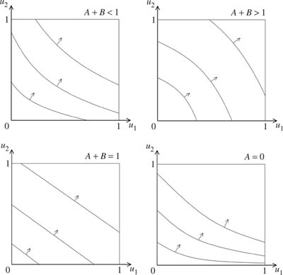
Figure 10.1. Separable preferences. The three cases considered in section 3.6.2 are illustrated, together with the case A = 0 that I suggest should be regarded as the norm. The utility function u is constant along the curves that have been drawn. Economists say these indifference curves are convex in the case A + B < 1 and concave in the case A + B > 1. In the case A = 0, Pandora is indifferent between all values of u1 with 0 ![]() u1
u1 ![]() 1 when u2 = 0.
1 when u2 = 0.
where Bc1 = u1 (c1) and Bc2 = u2 (c2). Thus,
u1 (c1)(Ac2 − 1) = u2 (c2)(Ac1 − 1),
and so Ac1 = Ju1 (c1) + 1 and Ac2 = Ju2 (c2) + 1 for some constant J.
It follows that any Von Neumann and Morgenstern utility function u that represents ![]() on lott(C) can be written in the form
on lott(C) can be written in the form
u(c1, c2) = Ju1 (c1)u2 (c2) + u1 (c1) + u2 (c2) + K.
To obtain the representation (3.3), simply renormalize u, u1, and u2 as in section 3.6.2. Figure 10.1 illustrates the three cases: A + B < 1, A + B = 1, and A + B > 1. It also shows what happens when A = 0, so that an absolute zero can be identified.
10.2 Hausdorff’s Paradox of the Sphere
The proof of Hausdorff’s paradox is beyond the scope of this book, but it isn’t hard to show that the three sets A, B, and C into which he partitions a sphere all have inner measure zero and outer measure one.
If ![]() , then we can find a measurable set F
, then we can find a measurable set F ![]() A with m(F) >
A with m(F) > ![]() a. The rotations that take A to B and C will take F to G and H, where m(G) = m(H) = m(F) >
a. The rotations that take A to B and C will take F to G and H, where m(G) = m(H) = m(F) > ![]() a. Since G
a. Since G ![]() B and H
B and H ![]() C, G and H can’t overlap, and so p(G
C, G and H can’t overlap, and so p(G ![]() H) = m(G) + m(H) > a. Hence
H) = m(G) + m(H) > a. Hence ![]() .
.
But A can be rotated onto B ![]() H, and so
H, and so ![]() . This contradiction implies that
. This contradiction implies that ![]() .
.
It remains to observe that ![]() , because B
, because B ![]() C is the complement of A in the sphere.
C is the complement of A in the sphere.
10.3 Conditioning on Zero-Probability Events
The geometric arguments of section 5.5.3 that show how problems can arise when trying to condition on a zero-probability event are illustrated in figure 10.2. Let E denote the event that a randomly chosen chord to a circle of radius r exceeds r. What is prob(E)?
The probability is ![]() . We begin with the observation that
. We begin with the observation that
![]()
where F denotes a member of a finite partition of the sample space B. A limiting case of this result is
![]()
where prob(E|θ) is the conditional probability that E is true given that the midpoint of a chord lies on a radius that makes an angle θ with a fixed axis. If the radius of the circle is r, and the distance from the center of the circle to the midpoint of a chord is x, then figure 10.2(a) shows that the length of the chord is ![]() . It follows that 2y < r if and only if
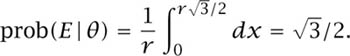
. It follows that 2y < r if and only if ![]() . If we assume that x is uniformly distributed on the radius, then
. If we assume that x is uniformly distributed on the radius, then
Substituting this result in (10.1), we find that prob![]() .
.
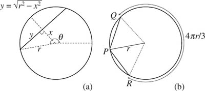
Figure 10.2. How long is a random chord? The left-hand diagram shows that a chord is longer than a radius if and only if ![]() . The right-hand diagram shows that a chord with one endpoint at P is longer than a radius if the other endpoint lies between Q and R. The longer arc joining Q and R has length 4πr/3.
. The right-hand diagram shows that a chord with one endpoint at P is longer than a radius if the other endpoint lies between Q and R. The longer arc joining Q and R has length 4πr/3.
The probability is ![]() . The alternative calculation is based on the formula
. The alternative calculation is based on the formula

where prob(E|x) is the conditional probability that E is true, given that the midpoint of a chord lies on a concentric circle of radius x. We therefore have that prob(E|x) = 0 unless ![]() .
.
The probability is ![]() . Figure 10.2(b) locates the endpoint of the chord that is chosen first at the point P. We then seek the value of prob(E|P).
. Figure 10.2(b) locates the endpoint of the chord that is chosen first at the point P. We then seek the value of prob(E|P).
If the other endpoint of the chord is placed at Q or R, then its length is equal to the radius. The arc of the circle between Q and R has length 4πr/3. Dividing by 2πr, we find that prob(E|P) = ![]() .
.
Which answer is right? There isn’t a one-and-only correct answer. In all three cases, we went beyond what the theory allows by assigning a value to a probability conditioned on a zero-probability event. We implicitly do this whenever we employ calculus in a probabilistic calculation, but how we do it should be understood as being part of our underlying model.
The first of the three cases best illustrates that it can matter how we proceed when following Kolmogorov’s advice to approximate the zero-probability event by events of positive probability. We can approximate the event of being on a particular radius in two ways, as illustrated in figure 10.3. We implicitly chose the first of these when we assumed that x was uniformly distributed on the radius, and so prob![]() . If we had chosen the second possibility, then
. If we had chosen the second possibility, then
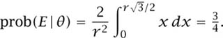

Figure 10.3. Kolmogorov’s advice. Kolmogorov recommends considering a sequence of events Fn with prob(Fn) > 0 that converges on a zero-probability event F. The figure shows two possible choices for events Fn that approximate a radius. The probability that the length of a random chord exceeds the length of a radius depends on the choice made.
10.4 Applying the Hahn–Banach Theorem
Section 6.4.3 claims that if Y is the vector space of almost convergent sequences and z lies outside Y, then p can be extended as a Banach limit from Y to z so as to make p(z) equal to any point w we like in the interval ![]() . To check that this is true, we appeal to the proof of the Hahn–Banach theorem with
. To check that this is true, we appeal to the proof of the Hahn–Banach theorem with ![]() . The reason that we need the extension of p to satisfy
. The reason that we need the extension of p to satisfy ![]() for all x is to ensure that the value of p(x) remains unchanged when we throw away a finite number of the terms of x. We can’t make do with less than this requirement, because of (6.12).
for all x is to ensure that the value of p(x) remains unchanged when we throw away a finite number of the terms of x. We can’t make do with less than this requirement, because of (6.12).
Recall that the extension is engineered one step at a time (section 6.4.2). When we extend p from Y to z by setting p(z) = w, we also need to extend p to the vector space Z spanned by Y and z. Any x in Z can be expressed uniquely in the form y + αz. Since a Banach limit is linear, our extension will need to have the property that p(y + αz) = p(y) + αp(z) for all α and all y. The question is then whether ![]() for all α and all y in Y.
for all α and all y in Y.
First observe that, for all y in Y,
![]()
![]()
![]()
When α ![]() 0, we then have that
0, we then have that
![]()
and when α ![]() 0,
0,
![]()
10.5 Muddling Boxes
Section 6.5 asserts that two different definitions of the upper and lower probability of a muddling box are the same. We consider only upper probabilities here, since the argument for lower probabilities is much the same. The proof we use is adapted from Goffman and Pedrick (1965, p. 68).
The first definition appears in section 6.4.3. The upper probability ![]() (x) of a sequence x whose terms lie in the interval [0, 1] is defined to be the smallest real number
(x) of a sequence x whose terms lie in the interval [0, 1] is defined to be the smallest real number ![]() for which it is true that for any
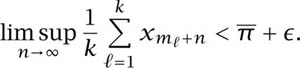
for which it is true that for any ![]() > 0, there exists N such that for any n > N and all values of m,
> 0, there exists N such that for any n > N and all values of m,
The second definition appears in section 6.5. The upper probability ![]() (x) of the sequence x is defined as
(x) of the sequence x is defined as
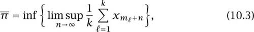
where the infimum ranges over all finite sets {m1, m2, . . . , mk} of natural numbers.
Proof that ![]() . Suppose that
. Suppose that ![]() > 0. For a large enough value of k and all values of m
> 0. For a large enough value of k and all values of m
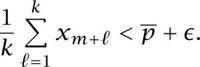
Take m1 = 1, m2 = 2, . . . , mk = k in (10.3). Then
Since ![]() for all
for all ![]() > 0, it follows that
> 0, it follows that ![]() .
.
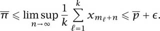
Proof that ![]() . Suppose that
. Suppose that ![]() > 0. We can find values of k, m1, m2, . . . , mk such that
> 0. We can find values of k, m1, m2, . . . , mk such that
Hence, there exists N such that for all n ![]() N,
N,
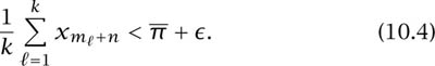
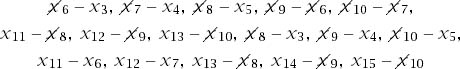
Figure 10.4. Cancelations. The figure expands the double summation that appears as the final term of (10.5) for the case n = 2, k = 2, m1 = 3, m2 = 5, i = 8. Only 6 + 10 = 2(m1 + m2) terms fail to cancel.
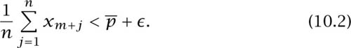
Replace n by n − N and ![]() , so that (10.4) then holds for all values of n. Write n + j for n in the left-hand side of the new inequality and average the result to get
, so that (10.4) then holds for all values of n. Write n + j for n in the left-hand side of the new inequality and average the result to get
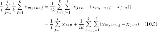
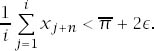
Figure 10.4 illustrates why cancelations in the concluding double summation leave only at most ![]() surviving terms. It follows that the double summation can be made smaller in modulus than
surviving terms. It follows that the double summation can be made smaller in modulus than ![]() by taking i sufficiently large.
by taking i sufficiently large.
It remains to observe that if i is sufficiently large,
Hence, for every ![]()
10.6 Solving a Functional Equation
Solving the functional equation f(xy) = f(x)f(y) for continuously differentiable real functions is a standard exercise in calculus. We first differentiate the equation partially with respect to y to obtain that xf′(xy) = f(x)f′(y). Writing y = 1 in this equation, we are led to the differential equation
![]()
where α = f′ (1). We need the derivative of f to be continuous in order to integrate this equation to obtain that
f(x) = Kxα,
for some constant K. Substituting this formula back into the functional equation with which we began, we find that K = 0 or K = 1.
Applying the same technique to the functional equation U(pq, PQ) = U(p, P)U(q, Q), we find that
U(p, P) = K(P)pα and U(p, P) = L(p)Pβ,
where α = U1 (1, 1) and β = U2 (1, 1). Thus
![]()
where c is an absolute constant.
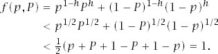
Since U(p, p) = p implies that c = 1 and α + β = 1, we find that the solution to our functional equation takes the form
U(p, P) = p1 − h Ph,
where the Hurwicz coefficient h satisfies ![]()
10.7 Additivity
Section 9.2.2 considers the behavior of π(E) + π(~E). For the case when ![]() and 0 < p < P < 1, we have that
and 0 < p < P < 1, we have that
To justify the first step, differentiate the left-hand side with respect to h to confirm that it is a strictly increasing function of h in the relevant range. To justify the second step, apply the inequality of the arithmetic and geometric means.
To confirm that there are cases with ![]() for which π(E) + π(~E) > 1, check that
for which π(E) + π(~E) > 1, check that ![]() for some values of p <
for some values of p < ![]() .
.
10.8 Muddled Equilibria in Game Theory
Section 9.3.1 describes some new Nash equilibria that arise in the Battle of the Sexes when muddled strategies are allowed. This section justifies these results.
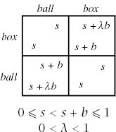
We work with the more general form of the Battle of the Sexes given in figure 10.5. The payoffs in this version of the game are to be interpreted as the probabilities of players winning win-or-lose lotteries in which losing corresponds to an absolute zero on their utility scales. Notice that the value of s is strategically significant when muddled strategies are used (although each of a player’s payoffs can be multiplied by the same positive factor without altering any strategic considerations).
For the mixed equilibrium, play your second pure strategy with probability
![]()
To secure your maximum payoff, play your second pure strategy with probability
![]()
Figure 10.5. A general version of the Battle of the Sexes. The payoffs are to be interpreted as probabilities of winning in win-or-lose lotteries in which losing corresponds to absolute zero on the player’s utility scale. The Battle of the Sexes of figure 9.5 is a scaled-up version of the case with s = 0, b = 1, and λ = ![]() . The text also analyzes the case s = b =
. The text also analyzes the case s = b = ![]() and λ =
and λ = ![]() .
.
The standard version of the Battle of the Sexes given in figure 9.5 corresponds to the case when s = 0 and λ = ![]() . The case when s = 0 and λ = 1 corresponds to the Driving Game. However, these cases are rather drastic since a failure to coordinate results in both players receiving their absolute zero. For everyday problems, we need to allow s to be positive (as in section 9.2.3).
. The case when s = 0 and λ = 1 corresponds to the Driving Game. However, these cases are rather drastic since a failure to coordinate results in both players receiving their absolute zero. For everyday problems, we need to allow s to be positive (as in section 9.2.3).
The analysis of the Battle of the Sexes given in section 9.3 generalizes to the version given in figure 10.5. There are two asymmetric pure Nash equilibria and a symmetric mixed Nash equilibrium. In the latter, both players use their second pure strategy with probability e = λ/(1 + λ). Their expected payoff is then c = s + eb, which is also their maximin value in the game. But the strategy that guarantees the maximin value requires that the second pure strategy be played with probability m = 1/(1 + λ). Since ![]() , the general version of the Battle of the Sexes generates the same problem in identifying a solution to the Battle of the Sexes in a symmetric environment that we encountered in section 9.3.
, the general version of the Battle of the Sexes generates the same problem in identifying a solution to the Battle of the Sexes in a symmetric environment that we encountered in section 9.3.
If Adam plays his second pure strategy with probability p and Eve plays her second pure strategy with probability q, then Adam’s payoff is
![]()
where c = s + bλ/(1 + λ) is the mixed equilibrium payoff (that each player gets when p = q = e). It is also the maximin payoff each player guarantees by playing p = m or q = m.
Plan of attack. The first item that needs to be proved is that the Battle of the Sexes has a continuum of symmetric Nash equilibria when muddled strategies are allowed. We assume that both Adam and Eve have the same Hurwicz coefficient h, which satisfies ![]() (It is easy to get results if
(It is easy to get results if ![]() but not very interesting.) We write α = 1 − h and β = h.
but not very interesting.) We write α = 1 − h and β = h.
Suppose that Eve uses a muddled strategy with upper probability ![]() and lower probability
and lower probability ![]() . In a symmetric equilibrium, Adam’s best reply will be the muddled strategy in which
. In a symmetric equilibrium, Adam’s best reply will be the muddled strategy in which ![]()
We will only look at muddled strategies for Eve for which Adam’s best reply in mixed strategies is p = ![]() . The next step is then to show that Adam gets the same payoff if he deviates from this mixed strategy to the muddled strategy in which
. The next step is then to show that Adam gets the same payoff if he deviates from this mixed strategy to the muddled strategy in which ![]() = p and
= p and ![]() This will require further restrictions on Eve’s muddled strategy, but we won’t worry about this second step until we have finished studying the question of Adam’s best reply in mixed strategies.
This will require further restrictions on Eve’s muddled strategy, but we won’t worry about this second step until we have finished studying the question of Adam’s best reply in mixed strategies.
Adam’s best reply in mixed strategies. Our first restriction on Eve’s choice of muddled strategy is that ![]() If we write y =
If we write y = ![]() − e < 0 and Y =
− e < 0 and Y = ![]() − e > 0, then Adam’s best reply in mixed strategies is found by locating the value of x = p − m in the range [−m, 1 − m] that maximizes
− e > 0, then Adam’s best reply in mixed strategies is found by locating the value of x = p − m in the range [−m, 1 − m] that maximizes

where A = c/b(1 + λ).
The plan is to fix y < 0 and Y > 0 so that the solution to Adam’s maximization problem is
![]()
It will then follow that p = x + m = y + e = ![]() .
.
Such a solution x to our maximization problem will necessarily satisfy x < 0 (because y < 0 and e < m). If x doesn’t occur at an endpoint of the admissible interval [−m, 1 − m], it can be found by differentiating {A − xy}α{A − xY}β with respect to x and setting the result equal to zero. The resulting x is given by
![]()
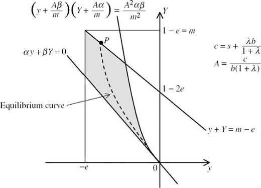
Figure 10.6. Muddled equilibria in the Battle of the Sexes. All points (y, Y) on the dashed curve correspond to symmetric Nash equilibria in muddled strategies. The point (0, 0) corresponds to the mixed Nash equilibrium. As we move (y, Y) away from (0, 0) along the dashed curve, the payoff to each player declines at first. However, there are parameter values for which the payoff to the players at the point P where the dashed curve crosses the boundary of the shaded set exceeds the payoff they get at the mixed equilibrium.
To make this conclusion compatible with our assumptions, we need to insist that
![]()
which is equivalent to the requirements that αy + βY > 0 and
![]()
These are two of the constraints on the pair (y, Y), as illustrated in figure 10.6. The constraints −e ![]() y < 0 and 0 < Y
y < 0 and 0 < Y ![]() 1 − e simply recognize that probabilities lie in [0, 1]. The constraint y + Y
1 − e simply recognize that probabilities lie in [0, 1]. The constraint y + Y ![]() m − e is explained later by inequality (10.10).
m − e is explained later by inequality (10.10).
Our restrictions on y and Y justify the claim that the value of x given by (10.7) maximizes Adam’s payoff for values of x in the interval [−m, 0], but what of the interval [0, 1 − m]? To show that (10.7) is also maximal when this interval is admitted, we need to use the fact that α ![]() β (because
β (because ![]() ). This inequality implies that (A − xY)α(A − xy)β decreases on [0, 1 − m], and hence is maximized at x = 0, where it is equal to (A − xy)α(A − xY)β.
). This inequality implies that (A − xY)α(A − xy)β decreases on [0, 1 − m], and hence is maximized at x = 0, where it is equal to (A − xy)α(A − xY)β.
Equilibrium condition. To make Adam’s best reply p = ![]() , we appeal to (10.7) and set
, we appeal to (10.7) and set
![]()
from which we obtain the equation
![]()
This equation defines the dashed curve in figure 10.6. The curve has a vertical asymptote y = −η for some positive value of η. On the interval (−η, 0], it lies above the line defined by αy + βY = 0 and beneath the branch of the hyperbola
![]()
drawn in figure 10.6.
Adam’s best reply in muddled strategies. If Eve chooses the muddled strategy corresponding to the pair (y, Y), we have found conditions under which it is a best reply for Adam to use the mixed strategy (x, X) = (y + e − m, y + e − m). We now show that it remains a best reply for Adam to use the muddled strategy (x, X) = (y + e − m, Y + e − m). The proof consists of showing that the deviation doesn’t affect Adam’s best or worst outcome, given that Eve has chosen (y, Y). For this purpose, we need the following inequalities:
Only the inequality A − (y + e − m)y ![]() A − (Y + e − m)Y fails to be satisfied whenever y < Y. To satisfy this exceptional inequality when y < Y, we need an extra condition:
A − (Y + e − m)Y fails to be satisfied whenever y < Y. To satisfy this exceptional inequality when y < Y, we need an extra condition:
![]()
This is the constraint illustrated in figure 10.6 that was left unexplained.
A continuum of muddled equilibria. Every pair (y, Y) on the dashed line in figure 10.6 that also lies to the right of the line y = −e and beneath the line y + Y = m − e corresponds to a symmetric Nash equilibrium in muddled strategies. A continuum of such equilibria therefore exists.
The case s = 0, b = 1, ![]() This is the case considered in figure 9.5, with the extra assumption that the players are uncertainty neutral
This is the case considered in figure 9.5, with the extra assumption that the players are uncertainty neutral ![]() The value of b only scales the payoffs up or down.
The value of b only scales the payoffs up or down.
In this case, the payoff to each player at the point P drawn in figure 10.6 is approximately 0.78. Each player uses a muddled strategy with lower probability approximately ![]() and upper probability approximately
and upper probability approximately ![]() .
.
The payoff pair (0.78, 0.78) is indicated in figure 9.7 by a star. It lies outside the mixed-strategy noncooperative payoff region of the Battle of the Sexes, because the highest payoff the players can get if both play the same mixed strategy is 0.75.
By continuity, similar results can be obtained for values of ![]() but one can’t reduce h very much before only symmetric equilibria with worse payoffs than the mixed equilibrium are left.
but one can’t reduce h very much before only symmetric equilibria with worse payoffs than the mixed equilibrium are left.
The case ![]() In this everyday case, the point P in figure 10.6 moves to the corner of the shaded region. At this equilibrium each player uses a muddled strategy with lower probability zero and upper probability one. The payoff to each player at the equilibrium is
In this everyday case, the point P in figure 10.6 moves to the corner of the shaded region. At this equilibrium each player uses a muddled strategy with lower probability zero and upper probability one. The payoff to each player at the equilibrium is ![]() which exceeds the payoff of
which exceeds the payoff of ![]() that each player gets at the mixed equilibrium.
that each player gets at the mixed equilibrium.
The Driving Game. Taking the limit as ![]() generates the Driving Game of figure 9.5. It is mentioned only to confirm that no new equilibria are created by allowing muddled strategies.
generates the Driving Game of figure 9.5. It is mentioned only to confirm that no new equilibria are created by allowing muddled strategies.