9

Large Worlds

9.1 Complete Ignorance

There was once a flourishing literature on rational decision theory in large worlds. Luce and Raiffa (1957, chapter 13) refer to this literature as decision making under complete ignorance. They classify what we now call Bayesian decision theory as decision making under partial ignorance (because Pandora can’t be completely ignorant if she is able to assign subjective probabilities to some events).

It says a lot about our academic culture that this literature should be all but forgotten. Presumably nobody reads Savage’s (1951) Foundations of Statistics any more, since the latter half of the book is entirely devoted to his own attempt to contribute to the literature on decision making under complete ignorance.

The principle of insufficient reason. The problems with this attempt to harness orthodox probability theory to the problem of making decisions under complete ignorance were briefly reviewed in section 7.4.3. Figure 9.1 provides an example in which the principle of insufficient reason chooses either action a₁ or action a₂.

Critics allow themselves much freedom in constructing examples that discredit the principle, but a more modest version wouldn’t be so easy to attack. For example, it is sometimes argued that our language—or the language in which we write our models—already incorporates implicit symmetries that would simply be made explicit if an appeal were made to a suitably restricted version of the principle of insufficient reason.

I am more enthusiastic about a much less ambitious proposal in which the class of traditional randomizing devices is expanded to other mechanisms for which it is possible to reject all reasons that might be given for regarding one outcome as more probable than another. One could then subsume such generalized lotteries into a theory of subjective probability in much the same way that traditional lotteries were subsumed in chapter 7. However, the need to explore all possible reasons for rejecting symmetry would seem incompatible with an assumption of complete ignorance.

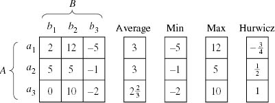
Figure 9.1. A decision problem. The diagram shows a specific decision problem D : A × B → C represented as in figure 1.1 by a matrix. In this case, the consequences that appear in the matrix are Von Neumann and Morgenstern utilities. The ancillary columns are to help determine the action chosen by various decision criteria. The principle of insufficient reason chooses a₁ or a₂. The maximin criterion chooses a₂. The Hurwicz criterion with chooses a₃.

The maximin criterion. We met the maximin criterion in section 3.7, where the idea that it represents nothing more than a limiting case of the Von Neumann and Morgenstern theory was denied. In figure 9.1, the maximin criterion chooses a₂.

A standard criticism of the maximin criterion is that it is too conservative. Suppose, for example, that Pandora is completely ignorant about how a number between 1 and 100 is to be selected. She now has to choose between two gambles, g₁ and g₂. In g₁, she wins $1m if the number 1 is selected and nothing otherwise. In g₂, she wins nothing if the number 100 is selected, and $1m otherwise. The gamble g₂ dominates g₁ because Pandora always gets at least as much from g₂ as g₁, and in some states of the world she gets more. But the maximin criterion tells her to be indifferent between the two gambles.

The Hurwicz criterion. Leo Hurwicz was a much-loved economist who lived a long and productive life, rounded off by the award of a Nobel prize for his work on mechanism design shortly before his death. He doubtless regarded the Hurwicz criterion as a mere jeu d’esprit. The criterion is a less conservative version of the maximin criterion in which Pandora evaluates an action by considering both its worst possible outcome and its best possible outcome. If c and C are the worst and the best payoffs she might get from choosing action a, Hurwicz (1951) suggested that Pandora should choose whichever action maximizes the value of

where the Hurwicz constant measures how optimistic or pessimistic Pandora may be. In figure 9.1, the Hurwicz criterion with chooses a₃. With h = 0, it chooses a₂ because it then reduces to the maximin criterion.

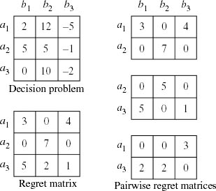
Figure 9.2. Minimax regret. The regret matrix is found by subtracting Pandora’s actual payoff at an outcome from the maximum payoff she could have gotten in that state if she had chosen another action. She is then assumed to apply the minimax criterion to her regret matrix. The pairwise regret matrices are supplied to help check that Pandora’s choices over pairs of actions reveal the intransitive preferences .

A more sophisticated version of the Hurwicz criterion known as alpha-max-min has been proposed, but the generalization I propose later goes in another direction (Ghirardato et al. 2004; Marinacci 2002).

The minimax regret criterion. Savage’s (1951) own proposal for making decisions under complete ignorance is the minimax regret criterion. Since he is one of our heroes, it is a pity that it isn’t easier to find something to say in its favor.

The criterion first requires replacing Pandora’s decision matrix of figure 9.1 by a regret matrix as in figure 9.2. The regrets are found by subtracting her actual payoff at an outcome from the maximum payoff she could have gotten in that state. She is then assumed to apply the minimax criterion (not the maximin criterion) to her regret matrix.¹

One could take issue with Savage for choosing to measure regret by subtracting Von Neumann and Morgenstern utilities, but he could respond with an argument like that of section 4.3. However, the failure of the minimax regret criterion to honor Houthakker’s axiom seems fatal (section 1.5.2). The example of figure 9.2 documents the failure. The minimax regret criterion requires Pandora to choose a₁ from the set A = {a₁, a₂, a₃}. But when she uses the minimax regret criterion to choose from the set B = {a₁, a₃}, she chooses a₃.

9.1.1 Milnor’s Axioms

John Milnor is famous for his classic book Differential Topology, but he was sufficiently interested in what his Princeton classmates like John Nash were doing that he wrote a paper on decision making under complete ignorance that characterizes all the criteria we have considered so far.

Milnor’s analysis uses the matrix representation of a decision problem D : A × B → C we first met in figure 1.1. The rows of the matrix represent actions in a feasible set A. The columns represent states of the world in the set B. As in figure 9.1, the consequences are taken to be Von Neumann and Morgenstern utilities.

For each such problem, Milnor assumes that Pandora has a preference relation defined over the set A of actions. He then considers ten different axioms that we might impose on this preference relation. These ten axioms appear as the rows of the table in figure 9.3, which preserves the names that Milnor gave to them. The columns correspond to the four decision criteria considered earlier in this section. The circles show when a criterion satisfies a particular axiom. The stars indicate axioms that characterize a criterion when taken together.

Milnor’s axioms are described below. Discussion of their significance is postponed until section 9.1.2.

1. Ordering. Pandora has a full and transitive preference relation over the actions in A.

2. Symmetry. Pandora doesn’t care how the actions or states are labeled.

3. Strong domination. If each entry in the row representing the action a_i strictly exceeds the corresponding entry in the row representing the action a_j, then Pandora strictly prefers a_i to a_j.

4. Continuity. Consider a sequence of decision problems with the same set of actions and states, in all of which . If the sequence of matrices of consequences converges, then its limiting value defines a new decision problem, in which .

5. Linearity. Pandora doesn’t change her preferences if we alter the zero and unit of the Von Neumann and Morgenstern utility scale used to describe the consequences.

6. Row adjunction. Pandora doesn’t change her preferences between the old actions if a new action becomes available.

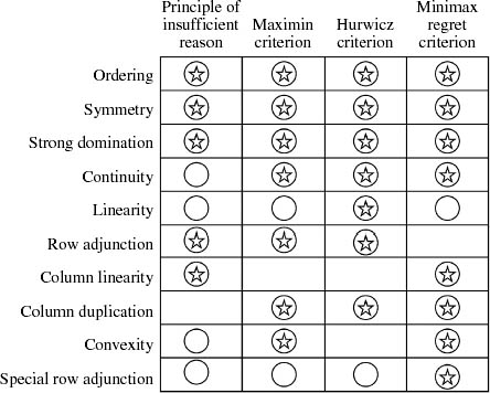
Figure 9.3. Milnor’s axioms. This table is reproduced from Milnor’s (1954) Games against Nature. The circles indicate properties that the criteria satisfy. The stars indicate properties that characterize a criterion when taken together.

7. Column linearity. Pandora doesn’t change her preferences if a constant is added to each consequence corresponding to a particular state.

8. Column duplication. Pandora doesn’t change her preferences if a new column is appended that is identical to one of the old columns.

9. Convexity. Pandora likes mixtures. If she is indifferent between a_i and a_j and an action is available that always averages their consequences, then she likes the average action at least as much as a_i or a_j.

10. Special row adjunction. Pandora doesn’t change her preferences between the old actions if a new action that is weakly dominated by all the old actions becomes available.

Implications of column duplication. It seems to me that we can’t do without axioms 1, 2, 3, 4, and 6, and so I shall call these the indispensable axioms. Savage’s minimax regret criterion is therefore eliminated immediately because it fails to satisfy axiom 6 (row adjunction).

The indispensable axioms imply two conclusions that will be taken for granted in what follows. The first conclusion is that axiom 4 (continuity) can be used to generate a version of axiom 3 (strong domination) without the two occurrences of the word strictly. The second conclusion is that axioms 1, 2, and 6 imply that the order in which entries appear in any row of the consequence matrix can be altered without changing Pandora’s preferences.

The axioms on which Milnor’s work invites us to focus are axiom 7 (column linearity) and axiom 8 (column duplication). Taken together with the indispensable axioms, column linearity implies the principle of insufficient reason. Column linearity is therefore much more powerful than it may appear at first sight. But if we are completely ignorant about the states of the world, why should we acquiesce in a principle that tells us that a column which is repeated twice corresponds to two different but equiprobable states of the world? Perhaps it is really the same column written down twice. Taking this thought to the extreme, we are led to axiom 8 (column duplication).

Along with the indispensable axioms, column duplication implies that Pandora’s preferences over actions depend only on the best and worst consequences in any row. To see why this is true, it is easiest to follow Milnor in identifying an action with the row of consequences to which it leads.

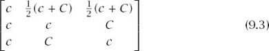
The two conclusions we have just derived from the indispensable axioms imply that

where the minimum of c₁, c₂, . . ., c_n is c and the maximum is C. We also need the second conclusion to infer that Pandora is indifferent between the two actions (c, C) and (C, c). It then follows that Pandora is indifferent between (c, c, . . ., C) and (C, C, . . ., c) because the first of the following matrices can be obtained from the second by column duplication:

The fact that Pandora is indifferent between all actions with the same best and worst outcomes can then be deduced from (9.2).

Characterizing the Hurwicz criterion. We have seen that the indispensable axioms plus column duplication imply that we need only consider actions of the form (c, C), where c C. To characterize the Hurwicz criterion, we also need axiom 5 (linearity). Most commentators would include linearity among the indispensable axioms, but I think there is good reason to be more skeptical (section 9.1.2).

To obtain the Hurwicz criterion, Milnor begins by defining the Hurwicz constant h to be the smallest number no smaller than any k for which (k, k) (0, 1). The continuity axiom then tells us that

(h, h) ~ (0, 1),

where 0 h 1 (by strong domination). For c < C, the linearity axiom then implies that

((C − c)h + c, (C − c)h + c) ~ (c, C).

Finding the best (c, C) is therefore the same as maximizing the Hurwicz expression: (1 − h)c + hC = (C − c)h + c.

Characterizing maximin. I think that axiom 9 (convexity) is misplaced among Milnor’s postulates. As with risk aversion, it tells us something about what Pandora happens to like, rather than how she must behave if she is to avoid irrationality. However, it suffices to ensure that h = 0 in the Hurwicz criterion.²

As previously, we need only consider actions of the form (c, C) with c C. Milnor now applies the convexity axiom to the matrix

to deduce that By repeating this argument over and over again with C replaced by and then appealing to axiom 4 (continuity), we are led to the conclusion that (c, C) (c, c). Weak domination then yields that (c, C) ~ (c, c). Finding the best (c, C) is therefore the same as maximizing c.

9.1.2 Discussion of Milnor’s Axioms

Milnor’s axioms treat Pandora’s preferences over actions as fundamental, but it is easy to recycle the arguments of chapter 1 so that his results can be absorbed into the theory of revealed preference. We simply treat Pandora’s choices between acts in the set of all acts as fundamental, and then use the preferences she reveals when these choices are consistent as the necessary input into Milnor’s theory. His axiom 6 (row adjunction) can then be replaced by Houtthaker’s axiom, which allows us to dispense with the need to assume transitivity of preference in his axiom 1 (ordering).

Milnor’s identification of the final consequences in a decision problem with Von Neumann and Morgenstern utilities also needs some consideration. He thereby implicitly assumes a version of our postulate 3, which allows a prize in a lottery to be replaced by any independent prize that Pandora likes equally well (section 3.4.1). We extended this postulate to gambles when developing Bayesian decision theory in section 7.2, and there seems no good reason for accepting it there but not here. In any case, section 6.4.1 has already signaled my intention of upholding this assumption even in the case of totally muddling boxes.

Linearity. Luce and Raiffa (1957, chapter 13) provide an excellent discussion of the background to Milnor’s axioms that is partly based on a commentary by Herman Chernov (1954). However, neither in their discussion nor anywhere else (as far as I know) is any serious challenge offered to Milnor’s axiom 5 (linearity), which says that we are always free to alter the zero and the unit on Pandora’s Von Neumann and Morgenstern utility scale without altering her preferences among actions. It is for this reason that time was taken out in section 3.6.2 to explain the circumstances under which it makes sense to identify an absolute zero on Pandora’s utility scale.

My reasons for arguing that the existence of an absolute zero should be treated as the default case become more pressing in a large-world context, and I therefore think it a mistake to insist on axiom 5 when contemplating decisions made under complete ignorance. But abandoning axiom 5 rules out all four of the decision criteria that appear in Milnor’s table of figure 9.3. However, we shall find that the Hurwicz criterion can be resuscitated in a multiplicative form rather than the classical additive form.

Separating preferences and beliefs? With the indispensable axioms, Milnor’s axiom 7 (column linearity) implies the principle of insufficient reason. The reasons for rejecting linearity apply with even greater force to column linearity, but abandoning axiom 7 entails a major sacrifice. Luce and Raiffa (1957, p. 290) make this point by noting that axiom 7 follows from Rubin’s axiom, which says that Pandora’s preferences over actions should remain unaltered if some random event after her choice of action might replace her original decision problem by a new decision problem whose consequence matrix has rows that are all the same, so that her choice of action is irrelevant.

Denying Rubin’s axiom as a general principle puts paid to any hopes we might have had of sustaining the purity of Aesop’s principle in a large world. The probability with which Pandora’s choice doesn’t matter would make no difference to her optimal choice if her preferences and beliefs were fully separated. We therefore have to learn to tolerate some muddling of the boundary between preferences and beliefs in a large world. A major virtue of Milnor’s axiom system is that it forces us to confront such inconsistencies between our different intuitions—rather as the Banach–Tarski paradox forces us to face up to similar inconsistencies in our intuitions about the nature of congruent sets in Euclidean space (section 5.2.1).

Taking account only of maxima and minima. We have seen that it is Milnor’s axiom 8 (column duplication) which allows us to escape being trapped in the principle of insufficient reason. It is easy to respond that column duplication is too strong an assumption, but I think such criticism overlooks Milnor’s insistence that he really is talking about making decisions under complete ignorance. On this subject, Milnor (1954, p. 49) says:

Our basic assumption that the player has absolutely no information about Nature may seem too restrictive. However such no-information games may be used as a normal form for a wider class of games in which certain types of partial information are allowed. For example if the information consists of bounds for the probabilities of the various states of Nature, then by considering only those mixed strategies for Nature which satisfy these bounds, we construct a new game having no information.

My approach in the rest of this chapter can be seen partly as an attempt to make good on this prognosis, with upper and lower probabilities serving as the bounds on the probabilities of the states of nature to which Milnor refers. In taking this line, I follow Klibanoff, Marinacci, and Mukerji (2005), who derive a version of the Hurwicz criterion by modifying the Von Neumann and Morgenstern postulates. However, I am more radical, since I abandon Milnor’s linearity axiom, which allows me to work with products of utilities rather than sums.

Convexity. I have already observed that Milnor’s axiom 9 (convexity) doesn’t belong in a list of rationality axioms. However, if one is going to make this kind of assumption it seems to me that one can equally well argue in favor of anti-convexity:³

9*. Anti-convexity. Pandora regards a mixture of two actions as optimal if and only if she also regards each of the two actions as optimal as well.

What happens to Milnor’s defense of the maximin criterion if we replace his axiom 9 by the new axiom 9*? Begin by switching the roles of c and C in the matrix (9.3). If the first row is optimal in the new matrix, then anti-convexity implies that the second and third rows are optimal too. If the first row isn’t optimal, then either the second or the third row is optimal. Either way, we find that Milnor’s argument then yields that (C, c) (C, C) and so we end up with the maximax criterion in place of the minimax criterion!

Something has obviously gone badly wrong here. We can even generate a contradiction by writing down the most natural version of axiom 9:

9**. Indifference to mixtures. If Pandora is indifferent between two actions, then she is indifferent between all mixtures of the actions.

This axiom is inconsistent with column duplication and the indispensable axioms, because it simultaneously implies both the maximin and maximax criteria.

I think our intuitions are led astray by pushing the analogy with lotteries too far. In particular, I don’t feel safe in making any a priori assumptions that say how Pandora should value mixtures of muddling boxes in terms of the muddling boxes that get mixed (section 6.4). To do so is to proceed as though nonmeasurable sets behave just like measurable sets.

9.2 Extending Bayesian Decision Theory

If Pandora isn’t ignorant at all, then she knows which state of the world applies in advance of making any decision. If she is completely ignorant, she decides without any information at all. There are many intermediate possibilities corresponding to all the different items of partial information that may be available to her—usually in a vague form that is difficult to formalize. Bayesianism holds that all such cases of partial ignorance can be dealt with by assigning unique subjective probabilities to the states of the world. I think that Bayesian decision theory only applies in small worlds in which Pandora’s level of ignorance can be regarded as being relatively low (section 7.1.1). So there is a gap waiting to be filled between the case of low partial ignorance and the case of total ignorance.

I now follow numerous others—notably Gilboa (2004) and Gilboa and Schmeidler (2001)—in trying to fill some of this gap, but without following the usual practice of proposing a system of axioms or postulates. This wouldn’t be hard to do, but I feel that the axiom–theorem–proof format stifles the kind of open-minded debate that is appropriate in such a speculative enterprise.

A minimal extension of Bayesian decision theory. I have no idea how to proceed if one isn’t allowed to appeal to Savage’s massaging process, so that Pandora can be supposed to have attained some level of consistency in her subjective beliefs (section 7.5.1). The large worlds to which my theory applies are therefore not the immensely large worlds that would need to be considered if we were aspiring to solve the problem of scientific induction. My worlds go beyond the Bayesian paradigm only to the extent that Pandora isn’t required to produce a determinate subjective probability for each and every event.

When massaging her initial snap judgments, Pandora may find that an event E about which she is ignorant must be assigned an upper probability (E) < 1 and a lower probability (E) > 0 for consistency reasons, but we don’t require that she tie her beliefs down any further (section 5.6). If she is completely ignorant, then (E) = 1 and (E) = 0.

One may argue that features of the event E that aren’t strictly probabilistic in character may also be relevant, so that factors other than (E) and (E) need to be taken into account in evaluating E. It is partly for this reason that muddling boxes were introduced in section 6.5. They are intended to provide an example of a case in which only the upper and lower probabilities of an event have any significance. Just as roulette wheels exemplify the kind of mechanism to which the models of classical probability theory apply, muddling boxes are intended to exemplify the kind of mechanism to which the calculus of upper and lower probabilities applies.

We saw in section 5.6.3 that Giron and Rios (1980) examined the extent to which Bayesian decision theory can be applied in such a situation. However, in their quasi-Bayesian theory, Pandora doesn’t have a full set of preferences over the set of acts. My theory goes further by postulating that she does have a full set of preferences over acts, even though her beliefs are incomplete in the Bayesian sense.

A price has to be paid for such an extension of the theory: we can no longer ask that Pandora’s beliefs over states in the set B can be fully separated from her preferences over consequences in the set C. One way to say this is that we follow Milnor in sacrificing his column linearity for column duplication (section 9.1.2).

9.2.1 Evaluating Nonmeasurable Events

In the following gamble G, Pandora gets the best possible prize if the event E occurs and the worst possible prize if the complementary event ~E occurs:

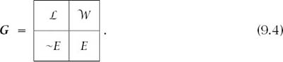
In section 7.2, we made assumptions that allowed a probability p(E) to be assigned to the event E, but we are now concerned with the case in which the event E isn’t measurable. However, other events are assumed to be measurable, so that it becomes meaningful to talk about the upper probability P = (E) and the lower probability p = (E) of the event E.

If we assume that the Von Neumann and Morgenstern postulates apply when the prizes in lotteries are allowed to be gambles of any kind, then we can describe Pandora’s choice behavior over such lotteries with a Von Neumann and Morgenstern utility function u, which we can normalize so that

The next step is then to accept the principle that motivates Milnor’s column duplication axiom by assuming that Pandora’s utility for the gamble G of (9.4) depends only on the upper and lower probabilities of E, so that we can write

Quasi-probability. Our normalization of the Von Neumann and Morgenstern utility function u makes it possible to regard u(G) not only as Pandora’s utility for a particular kind of gamble, but also as a kind of quasi-probability of the event E. When doing so, I shall write

Although the assumptions to be made will result in π turning out to be nonadditive, I shan’t call it a nonadditive probability as is common in the literature for analogous notions (section 5.6.3). I think this would be too misleading for a theory that doesn’t involve computing generalized expected values of any kind (whether using the Choquet integral or not). To evaluate a gamble like

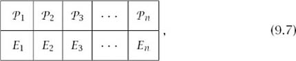
Pandora will be assumed to begin by replacing each consequence by an independent win-or-lose lottery that she likes equally well. She then works out the event F in which she will get the best prize in the resulting compound gamble. Her final step is to choose a feasible gamble that maximizes the value of

These remarks aren’t meant to imply that the various theories of non-additive probability that have been proposed have no applications. A theory that dealt adequately with all the ways in which Pandora might be partially ignorant would presumably need to be substantially more complicated than the theory I am proposing here.

9.2.2 The Multiplicative Hurwicz Criterion

What properties should be attributed to the function U? The following assumptions seem uncontroversial:

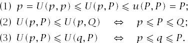
The second and third assumptions are reminiscent of the separable preferences discussed in section 3.6.2. The analogy can be pushed much further by considering Pandora’s attitude to independent events.

The rest of this section argues that we can thereby justify the use of a multiplicative Hurwicz criterion in which U takes the form

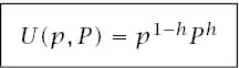
The constant will be called a (multiplicative) Hurwicz coefficient.

Independence. If a roulette wheel is spun twice, everybody agrees that the slot in which the little ball stops on the first spin is independent of the slot on which it stops on the second spin. If s₁ is the slot that results from the first spin and s₂ is the slot that results from the second spin, then we write (s₁, s₂) to represent the state of the world in which both spins are considered together. The set of all such pairs of states is denoted by S₁ × S₂, where S₁ is the set of all states than can arise at the first spin and S₂ is the set of all states that can arise at the second spin.

More generally, suppose that B = B₁ × B₂, where it is understood that all events E in B₁ are independent of all events F in B₂. The plan is to look at Pandora’s attitude to the set of all events E × F. We suppose that

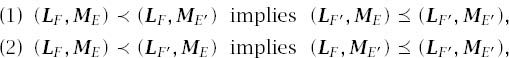
where the lotteries L_F and M_E are of the type indicated in figure 9.4.

We can now recycle the argument of section 3.6.2 to obtain an equation analogous to (3.3):

Since and we obtain that

where the events E and F have been identified with E × B₂ and B₁ × F.

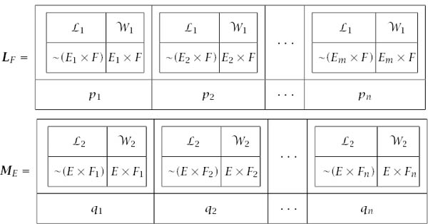
Figure 9.4. Some lotteries. The prizes in lotteries of type L_F incorporate different E_i but always have the same F. The prizes in lotteries of type M_E incorporate different F_j but always have the same E.

To go further, we rewrite (9.8) in terms of the function U. For this purpose, take and But and and so we are led to the functional equation

Such functional equations are hard to satisfy. The only continuously differentiable solutions take the multiplicative form

that we have been seeking to establish (section 10.6).

Additivity? Because (section 5.6.2), it is always true that

with equality only in the measurable case when More generally,

for all events E if and only if (section 10.7). If , then π(E) + π(~E) = 1 if and only if

The case when isn’t symmetric because the inequality of the arithmetic and geometric means says that

with equality if and only if p = P.

Absolute zero. If then π(E) = 0 no matter what the value of may be. It is for this reason that the case of an absolute zero was discussed in section 3.6.2. However, in everyday decision problems, the existence of an absolute zero is unlikely to upset any standard intuitions. The following application of the multiplicative Hurwicz criterion to the Ellsberg paradox provides an example.

9.2.3 Uncertainty Aversion

The Ellsberg paradox is explained in figure 5.2. Subjects in laboratory experiments commonly reveal the preferences

but there isn’t any way of assigning subjective probabilities to the variously colored balls that makes these choices consistent with maximizing expected utility. Such behavior is usually explained by saying that most people are averse to ambiguity or uncertainty in a manner that is incompatible with Bayesian decision theory.⁴ However, the behavior is compatible with the minimal extension considered here.

To see why, suppose that Pandora is indifferent between winning one million dollars in an Ellsberg lottery and participating in a lottery in which she gets her best possible outcome with probability b and her worst possible outcome with probability 1 − b. Suppose she is also indifferent between losing and participating in a lottery in which she gets with probability s and with probability 1 − s, where b > s. If > 0 is small and b/s = 1 + , then

In everyday decision problems, Pandora will therefore reveal preferences that are uncertainty averse whenever the Hurwicz coefficient For this reason, I think that the case when is only of limited interest.

9.2.4 Bayesian Updating

How does one update upper and lower probabilities after receiving a new piece of information (Klibanoff and Hanany 2007)? There seems to be nothing approaching a consensus in the literature on a simple formula that relates the prior upper and lower probabilities with the posterior upper and lower probabilities. Observing a new piece of information may even lead Pandora to expand her class of measurable sets so that all her subjective probabilities need to be recalculated from scratch.

However, if we restrict our attention to the special case discussed in section 8.4.2, matters become very simple. If Pandora never has to condition on events F other than truisms to which she can attach a unique probability, then we can write

9.3 Muddled Strategies in Game Theory

Anyone who proposes a decision theory that distinguishes between risk and uncertainty naturally considers the possibility that it might have interesting applications in game theory.⁵ Because of the way my own theory treats independence, it is especially well adapted for this purpose.

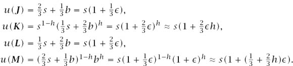
Mixed strategies. If a game has a rational solution, it must be one of the game’s Nash equilibria (section 2.2). In figure 2.1, the cells of the payoff tables in which both payoffs are circled correspond to Nash equilibria, because each player is then making a best reply to the strategy choice of the other. However, in the game Matching Pennies of figure 9.5, none of the cells have both their payoffs circled. It follows that Matching Pennies has no Nash equilibrium in pure strategies.

To solve games like Matching Pennies, we need to extend the class of pure strategies to a wider class of mixed strategies—an idea of Von Neumann that was anticipated by the mathematician Émile Borel. A mixed strategy requires that players use a random device to choose one of their pure strategies with predetermined probabilities. For example, if Alice bluffs with probability when holding the Jack in Mini-Poker, she is using a mixed strategy (section 8.3.1).

In Matching Pennies, it is a Nash equilibrium if each player uses the mixed strategy in which heads and tails are played with equal probability. They are then using the maximin strategy that Von Neumann identified as the rational solution of such two-person zero-sum games.

John Nash showed that all finite games have at least one Nash equilibrium when mixed strategies are allowed, but his result doesn’t imply that the problem of identifying a rational solution of an arbitrary game is solved. Aside from other considerations, most games have many equilibria. Deciding which equilibrium will be played by rational players is one aspect of what game theorists call the equilibrium selection problem.

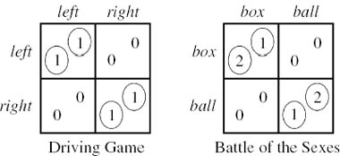
Figure 9.5. Two games. Matching Pennies has a mixed Nash equilibrium in which Alice and Bob both choose heads or tails with probability . The Battle of the Sexes has two Nash equilibria in pure strategies. Like all symmetric games, it also has a symmetric equilibrium in which both players use their second pure strategy with probability . At this equilibrium each player gets only their security level. However, to guarantee their security levels, each player must use their second pure strategy with probability .

Battle of the Sexes. The Battle of the Sexes of figure 9.5 is an example invented by Harold Kuhn to illustrate how intractable the equilibrium selection problem can be, even in very simple cases.⁶

The politically incorrect story that goes with this game envisages that Adam and Eve are honeymooning in New York. At breakfast, they discuss where they should meet up if they get separated during the day. Adam suggests that they plan to meet at that evening’s boxing match. Eve suggests a performance of Swan Lake. Rather than spoil their honeymoon with an argument, they leave the question unsettled. So when they later get separated in the crowds, each has to decide independently whether to go to the boxing match or the ballet. The Battle of the Sexes represents their joint dilemma.

The circled payoffs in figure 9.5 show that the game has two Nash equilibria in pure strategies: (box, box) and (ball, ball). All symmetric games have at least one symmetric Nash equilibrium when mixed strategies are allowed. The Battle of the Sexes has a unique symmetric equilibrium, whose properties are made evident by the right-hand diagram of figure 9.6.

The horizontal chord shows all payoff pairs that are possible if Adam plays his second pure strategy with probability p = . All of Eve’s strategies are best replies to this choice of mixed strategy by Adam. In particular, it is a best reply if she forces the outcome of the game to lie on the vertical chord of figure 9.6 by playing her second pure strategy with probability q = . All of Adam’s strategies are best replies to this mixed strategy, including p = . We have therefore found a mixed Nash equilibrium in which Adam plays p = and Eve plays q = . In this symmetric equilibrium, each player ends up with an expected payoff of .

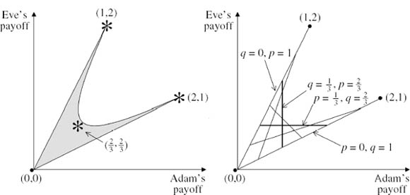
Figure 9.6. Battle of the Sexes. The very nonconvex set shaded in the left-hand diagram is the noncooperative payoff region of the Battle of the Sexes. It consists of all payoff pairs that can be achieved if Adam and Eve choose their mixed strategies independently. The stars show the payoff pairs at the three Nash equilibria of the game. The chords in the right diagram can be thought of as representing the players’ mixed strategies. Those drawn consist of all multiples of p = and q = , where p is the probability with which Adam chooses ball, and q is the probability with which Eve chooses box. As p takes all values between 0 and 1, the corresponding chord sweeps out the game’s noncooperative payoff region. The mixed Nash equilibrium of the game occurs where the horizontal chord corresponding to p = crosses the vertical chord corresponding to q = .

Solving the Battle of the Sexes? What is the rational solution of the Battle of the Sexes? If the question has an answer, it must be one of the game’s Nash equilibria. If we ask for a solution that depends only on the strategic structure of the game, then the solution of a symmetric game like the Battle of the Sexes must be a symmetric Nash equilibrium.⁷ Can we therefore say that the rational solution of the Battle of the Sexes requires that each player should use their second pure strategy with probability ?

The problem with this attempt to solve the Battle of the Sexes is that it gives both players an expected payoff of no more than , which also happens to be their maximin payoff—the largest expected utility a player can guarantee independently of the strategy used by the other player. However, Adam and Eve’s maximin strategies aren’t the same as their equilibrium strategies. To guarantee an expected payoff of , Adam must choose p = , which makes the corresponding chord vertical in figure 9.6. Eve must choose q = , which makes the corresponding chord horizontal.

This consideration undercuts the argument offered in favor of the symmetric Nash equilibrium as the solution of the game. If Adam and Eve are only expecting an expected payoff of from playing the symmetric Nash equilibrium, why don’t they switch to playing their maximin strategies instead? The payoff of they are expecting would then be guaranteed. At one time, John Harsanyi (1964, 1966) argued that the rational solution of the Battle of the Sexes therefore requires that Adam and Eve should play their maximin strategies.

Harsanyi’s suggestion would make good sense if the Battle of the Sexes were a zero-sum game like Matching Pennies, since it would then be a Nash equilibrium for Adam and Eve to play their maximin strategies. But it isn’t a Nash equilibrium for them to play their maximin strategies in the Battle of the Sexes. For example, if Adam plays p = , Eve’s best reply is q = 0.

The problem isn’t unique to the Battle of the Sexes (Aumann and Maschler 1972). If we are willing to face the extra complexity posed by asymmetric games, we can even write down 2 × 2 examples with a unique Nash equilibrium in which one of the players gets no more than his or her maximin payoff.

My plan is to use this old problem to illustrate why it can sometimes be useful to expand the class of mixed strategies to a wider class of muddled strategies in the same kind of way that Borel expanded the class of pure strategies to the class of mixed strategies.

9.3.1 Muddled Strategies

To implement a mixed strategy, players are assumed to use a randomizing device like a roulette wheel or a deck of cards. To implement a muddled strategy, they use muddling boxes (section 6.5).

In the Battle of the Sexes, a muddled strategy for Adam is therefore described by specifying the lower probability p and the upper probability P with which he will play his second pure strategy. A muddled strategy for Eve is similarly described by specifying the upper probability Q and the lower probability q with which she will play her second pure strategy.

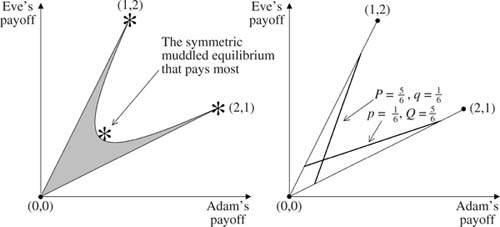
Figure 9.7. A muddled equilibrium in the Battle of the Sexes. In the case h = , there is a symmetric Nash equilibrium in which each player uses a muddled strategy with lower probability approximately and upper probability approximately . The equilibrium payoff to each player exceeds .

When muddled strategies are used in the Battle of the Sexes, I shall assume that the players’ preferences are determined by the multiplicative Hurwicz criterion (section 9.2.2). The Hurwicz coefficient h will be assumed to be the same for both players in order to keep everything symmetric. It will also be assumed that neither player likes uncertainty, so 0 h (section 9.2.3). We will get nothing new if h = 0, and so the case when the Hurwicz criterion reduces to the maximin criterion is excluded as well. Under these conditions, section 10.7 proves a number of results. In particular:

Figure 9.7 illustrates the case when h = . The symmetric equilibrium that pays most then requires that both players use a muddled strategy whose upper probability is approximately and whose lower probability is approximately . The payoff to each player at this equilibrium exceeds , and hence lies outside the noncooperative payoff region when only mixed strategies are allowed. In particular, both players get more than their maximin payoff of at this symmetric equilibrium.

It would be nice if this last result were true whenever h , but it holds only for values of h sufficiently close to . So the general problem of finding a rational solution to the Battle of the Sexes in a symmetric environment remains open.

9.4 Conclusion

This book follows Savage in arguing that Bayesian decision theory is applicable only in worlds much smaller than those in which it is standardly applied in economics. This chapter describes my own attempt to extend the theory to somewhat larger worlds. Although the extension is minimal in character, it nevertheless turns out that even very simple games can have new Nash equilibria if the players use the muddled strategies that my theory allows. I don’t know how important this result is for game theory in general. Nor do I know to what extent the larger worlds to which my theory applies are an adequate representation of the economic realities to which Bayesian decision theory has been applied in the past. Perhaps others will explore these questions, but I fear that Bayesianism will roll on regardless.

¹ Much confusion can be avoided by remembering that economists usually evaluate consequences in terms of gains and so apply the maximin criterion. Statisticians usually evaluate consequences in terms of losses and so apply the minimax criterion.

² Milnor’s characterization of the maximin criterion is only one of many. Perhaps the most interesting alternative is Barbara and Jackson (1988).

³ Axiom 9* follows from Rubin’s axiom, symmetry, and row adjunction.

⁴ See, for example, Dow and Werlang (1992), Epstein (1999, 2001), and Ryan (2002).

⁵ See, for example, Dow and Werlang (1994), Greenberg (2000), Lo (1996, 1999), Kelsey and Eichberger (2000), Marinacci (2000), and Mukerji and Shin (2002).

⁶ For a more extensive discussion of the classical game, see Luce and Raiffa (1957, p. 90).

⁷ The Driving Game is solved in the United States by choosing the asymmetric Nash equilibrium in which everybody drives on the right. This solution depends on the context in which the game is played, and not just on the strategic structure of the game. For example, the game is solved in Japan by having everybody drive on the left.