5

Classical Probability

5.1 Origins

Probability doesn’t come naturally to the human species. The ancients never came up with the idea at all, although they enjoyed gambling games just as much as we do. It was only in the seventeenth century that probability saw the light of day. The Chevalier de Méré will always be remembered for proposing a problem about gambling odds that succeeded in engaging the attention of two great mathematicians of the day, Pierre de Fermat and Blaise Pascal. Some of the letters they exchanged in 1654 still survive.¹ It is fascinating to learn how difficult they found ideas that we teach to school children as though they were entirely unproblematic.

Ian Hacking’s (1975) Emergence of Probability documents how the pioneering work of Fermat and Pascal was pursued by a galaxy of famous mathematicians, including Jacob Bernoulli, Huygens, Laplace and de Moivre. It is generally thought that the classical theory of probability was finally brought to a state of perfection in 1933 when Kolmogorov (1950) formulated the system of axioms that bears his name.

We took Kolmogorov’s formulation of probability theory for granted when presenting Von Neumann and Morgenstern’s theory of expected utility (section 3.4). However, in seeking a theory of decision that applies more widely, I need to explore the implicit assumptions built into Kolmogorov’s axioms. In taking on this task, the current chapter says nothing that mathematicians or statisticians will find unorthodox, but its focus is on interpretive questions that aren’t normally discussed very much, rather than on the mathematics of the theory.

5.2 Measurable Sets

The prosaic attitude of statisticians to probability is reflected in the language they use. In this book, the set B in a decision problem D : A × B → C is usually said to be the set of states of the world. Philosophers sometimes call B the universe of discourse. Statisticians call B a sample space.

The subsets of a sample space B are identified with possible events. For example, the sample space when a roulette wheel is spun is usually taken to be the set {0, 1, 2, 3, . . . , 36} of possible numbers that may come up.² The event that the number is odd is the subset {1, 3, 5, . . . , 35}.

It hasn’t mattered very much so far whether the set B is finite or infinite, but from now on it will be important not to exclude the possibility that it is infinite. Allowing B to be infinite creates various problems that some authors seek to exclude by insisting that only finite sets exist in the real world. Perhaps they are right, but our models aren’t the real world—they are always a draconian simplification of whatever the real world may be. Allowing infinite sets into our models is often part of the process of simplification, as when Isaac Newton modeled space and time as continuous variables to which his newly minted calculus could be applied.

In decision theory, there are even more pressing reasons for allowing an infinite number of states of the world. For example, the world we are trying to model in game theory sometimes includes the minds of the other players. When thinking about how to play, they may do some calculations. Do we want to restrict them to using only numbers smaller than some upper bound? When advising Alice, do we want to assume that her model of the world is sufficient to encompass all the models that Bob might be using, but not that Bob’s model is sufficient to encompass all the models that Alice might be using?

The last point takes us into even deeper waters. Do we really want to proceed as though we are capable of making a finite list of all relevant possibilities in any situation that might conceivably arise? I think this is demonstrably impossible even if we allow ourselves an infinite number of states (section 8.4). As Hamlet says to Horatio: “There are more things in heaven and earth, Horatio, than are dreamt of in your philosophy.” In brief, we need to avoid fooling ourselves into thinking that we always know how to scale down the universe into a manageable package.

The latter problem is captured in classical probability theory by saying that some events are measurable and others are not. The measurable events are those that we can tie down sufficiently to make it meaningful to attach a probability to them. To speak of the probability of a nonmeasurable set is to call upon the theory to deliver something for which it is unequipped.

In later chapters, I shall be arguing that one can’t follow the traditional practice of ignoring the possible existence of nonmeasurable sets when seeking to make rational decisions in a large world. However, it is difficult to get a feeling for the extent to which nonmeasurable sets can differ from their measurable cousins when they are only discussed in the abstract. It is therefore worth reviewing some of the examples that arise in Euclidean geometry.

5.2.1 Lebesgue Measure

Henri Lebesgue created the subject of measure theory when he showed how the concept of length can be extended to the class of Lebesgue measurable sets on the real line. In offering a potted explanation of his idea, I shall talk about the length of arcs on a given circle rather than the length of intervals on a line, because it is then possible to make the measure that results into a probability measure by normalizing so that the arc length of the whole circle is one. If you like, you can think of the circle as a generalized roulette wheel.

Lebesgue’s basic idea is simple. He saw that one can always use any collection C of measurable sets on a circle—sets to which one has already found a way of attaching an arc length—to find more measurable sets.

Suppose that S is contained in a set T in the collection C. If S is measurable, its measure m(S) can’t be more than m(T). In fact,

where is the largest real number no larger than all m(T) for which .

Similarly, if S contains a set T in the collection C, then m(S) can’t be less than m(T). In fact,

where is the smallest real number no smaller than all m(T) for which .

For some sets S, it will be true that

It then makes sense to say that S is measurable, and that its Lebesgue measure m(S) is the common value of and .

In the case of Lebesgue measure on a circle, it is enough to begin with a collection C whose constituent sets are all unions of nonoverlapping open arcs. The measure of such a set is taken to be the sum of the lengths of all the arcs in this countable collection.³ The sets that satisfy (5.3) with this choice of C exhaust the class of all Lebesgue measurable sets on the circle. Replacing C by in an attempt to extend the class of measurable sets just brings us back to again.

What do Lebesgue measurable sets look like? Roughly speaking, the answer is that any set that can be specified with a formula that uses the standard language of mathematics is Lebesgue measurable.⁴ Nonmeasurable sets are therefore sets that our available language is inadequate to describe. But do such sets really make sense in concrete situations?

Vitali’s nonmeasurable set. Vitali’s proof of the existence of a set on the circle that isn’t Lebesgue measurable goes like this.

We first say that two points on the circle are to be included in the same class if the acute angle they subtend at the center is a rational number.⁵ There are many such equivalence classes, but they never have a point in common. The next step is to make a set P by choosing precisely one point from each class. We suppose that P has measure m and seek a contradiction.

Let P_a be the set obtained by rotating P around the center of the circle through an acute angle a. The construction ensures that the collection of all P_r for which r is a rational number partitions the circle. This means that no two sets in the collection overlap, and that its union is the whole circle. It follows that the measure of the whole circle is equal to the sum of the measures of each member of the partition.

But all the sets in the partition are rotations of P, and so have the same measure m as P. The measure of the whole circle must therefore either be zero if m = 0, or infinity if m > 0. Since the measure of the whole circle is one, we have a contradiction, and so P is nonmeasurable.

The Horatio principle. The nonmeasurable set P is obtained by picking a point from each of the equivalence classes with which the proof begins, but no hint is offered on precisely how each point is to be chosen. In fact, to justify this step in the proof, an appeal needs to be made to the axiom of choice, which set theorists invented for precisely this kind of purpose. But is the axiom of choice true?

I think it fruitless to ask such metaphysical questions. The real issue is whether a model in which we assume the axiom of choice better fits the issues we are seeking to address than a model in which the axiom of choice is denied. We are free to go either way, because it is known that the axiom of choice is independent of the other axioms of set theory. Moreover, if we deny the axiom of choice, Robert Solovay (1970) has shown that we can then consistently assume that all sets on the circle are Lebesgue measurable.⁶

My own view is that to deny the axiom of choice in a large-world setting is to abandon all pretence at taking the issues seriously. It can be interpreted as saying that nature has ways of making choices that we can’t describe using whatever language is available to us. In a sufficiently complex world, the implication is that some version of what I shall call the Horatio principle must apply:

Some events in a large world are necessarily nonmeasurable.

The Banach–Tarski paradox. The properties of nonmeasurable sets become even more paradoxical when we move from circles to spheres (Wagon 1985).

Felix Hausdorff showed that we can partition the sphere into three sets, each of which can be rotated onto any one of the others. There is nothing remarkable in this, but each of his sets can also be rotated onto the union of the other two! If one of Hausdorff’s sets were Lebesgue measurable, its measure would therefore need to be equal to twice itself.

The Banach–Tarski paradox is even more bizarre. It says that a sphere can be partitioned into a finite number of nonoverlapping subsets that can be reassembled to make two distinct spheres, each of which is identical to the original sphere. Perhaps this is how God created Eve from Adam’s rib!

5.3 Kolmogorov’s Axioms

Kolmogorov’s formulation of classical probability theory is entirely abstract. Measurable events are simply sets with certain properties. A probability measure is simply a certain kind of function. Kolmogorov doesn’t insist on any particular interpretation of his theory, whether metaphysical or otherwise. His attitude is that of a pure mathematician. If we can find a model to which his theory applies, then we are entitled to apply all of his theorems in our model.

Abstract measurable sets. Kolmogorov first requires that one can never create a nonmeasurable set by putting his abstract measurable events together in various ways using elementary logic. He therefore makes the following assumptions.

1. The whole sample space is measurable.

2. If an event is measurable, then so is its complement.

3. If each of a finite collection of events is measurable, then so is their union.

I have listed these formal requirements only because Kolmogorov’s theory requires that the third item be extended to the case of infinite but countable unions:

3*. If each of a countable collection of events is measurable, then so is their union.

A set is countable if it can be counted. To count a set is to arrange it in a sequence, so that we can assign 1 to its first term, 2 to its second term, 3 to its third term, and so on. The infinite set of all natural numbers can obviously be counted. We used the fact that the set of all rational numbers is countable in section 1.7. The set of all real numbers is uncountable. No matter how we try to arrange the real numbers in a sequence, there will always be real numbers that are left out.

A mundane nonmeasurable set. After seeing Vitali’s construction of a set on the circle that isn’t Lebesgue measurable, it is natural to think that a nonmeasurable set must be a very strange object indeed, but Kolmogorov’s definition allows the most innocent of sets to be nonmeasurable.

Suppose, for example, that Pandora tosses a coin. The coin may have been tossed many times before and perhaps will be tossed many times again, but we don’t know anything about the future or the past. If we took our sample space B to be all finite sequences of heads and tails, with Pandora’s current toss located at some privileged spot in the sequence, then we might take account of our ignorance by only allowing the measurable sets to be Ø, H, T, and B, where H is the event that Pandora’s current toss is heads and T is the event that her current toss is tails.

The event that some previous toss of the coin was heads is then non-measurable in this setup. Of course, other models could be constructed in which the same event is measurable. As with so much else, such considerations are all relative to the model one chooses to adopt.

5.3.1 Abstract Probability

Kolmogorov defines a probability space to be a collection of measurable events from a sample space B together with a probability measure

It will be important not to forget that the theory only defines probabilities on measurable sets.⁷ The requirements for a probability measure are:

1. For any E, prob(E) 0 with equality for the impossible event E = Ø.

2. For any E, prob(E) 1 with equality for the certain event E = B.

3. If no two of the countable collection of events E₁, E₂, . . . have a state in common, then the probability of their union is

The union corresponds to the event that at least one of the events E₁, E₂, . . . occurs. Item 3 therefore says that we should add the probabilities of exclusive events to get the probability that one of them will occur.

Countable additivity? The third requirement for a probability measure is called countable additivity. It is the focus of much debate among scholars who either hope to generalize classical probability theory in a meaningful way, or else feel that they know the one-and-only true interpretation of probability. The former seek to extend the class of probability functions by exploring the implications of replacing countable additivity by finite additivity. The latter class of scholars has a distinguished representative in the person of Bruno de Finetti (1974b, p. 343), who tells us in capital letters that he REJECTS countable additivity.

Although de Finetti was a man of genius, we need not follow him in rejecting countable additivity for what seem to me metaphysical reasons. But nor do we need to hold fast to countable additivity if it stands in our way. Different applications sometimes require different models. Where we can’t have countable additivity, we must make do with finite additivity.⁸

There is an unfortunate problem about nomenclature when probabilities are allowed to be only finitely additive. A common solution is to talk about finitely additive measures, disregarding the fact that measures are necessarily countably additive by definition. The alternative is to invent a new word for a finitely additive function μ for which μ(Ø) = 0. I somewhat reluctantly follow Rao and Rao (1983) and Marinacci and Montrucchio (2004) in calling such a function a charge, but without any intention of using more than a smattering of their mathematical developments of the subject.

However, abandoning countable additivity is a major sacrifice. Useful infinite models can usually be regarded as limiting cases of the complex finite models that they are intended to approximate. In such cases, we don’t want “discontinuities at infinity” as a mathematician might say. The object in an infinite model that supposedly approximates an object in a complex finite model must indeed be an approximation to that object. In the case of probability theory, such a continuity requirement can’t be satisfied unless we insist that the probability of the limit of a sequence of measurable sets is equal to the limit of their individual probabilities.⁹ But countable additivity reduces to precisely this requirement.

This is only one reason that enthusiasts for finite additivity who think that junking countable additivity will necessarily make their lives easier are mistaken. We certainly can’t eliminate the problem of nonmeasurable sets in this way. It is true that we can find a finitely additive extension of Lebesgue measure to all sets on a circle, but Hausdorff’s paradox of the sphere shows that the problem returns to haunt us as soon as we move up to three dimensions.

5.4 Probability on the Natural Numbers

When people say that a point is equally likely to be anywhere on a circle, they usually mean that its location is uniformly distributed on the circle. This means that the probability of finding the point in a Lebesgue measurable set E is proportional to the Lebesgue measure of E. If E isn’t measurable, we are able to say nothing at all.

It is a perennial problem that classical probability theory doesn’t allow a uniform distribution on the real line. There is equally no probability measure p defined on the set of natural numbers with If there were, then

would have to be either 0 or + ∞, but . It is sometimes suggested that we should abandon the requirement that prob in order to escape this problem, but I think we would then throw the baby out with the bathwater.

De Finetti’s (1974a, 1974b) solution is bound up with his rejection of countable additivity. With finite additivity one can have 0 = p(1) = p(2) = p(3) = . . . without having to face the contradiction 1 = 0 + 0 + 0 + . . . (Kadane and O’Hagan 1995).

I don’t share de Finetti’s enthusiasm for rejecting countable additivity, but one can’t but agree that we have to do without it when situations arise in which each natural number needs to be treated as equally likely. However, de Finetti wouldn’t have approved at all of my applying the idea to objective probabilities in the next chapter.

5.5 Conditional Probability

Kolmogorov introduces conditional probability as a definition:

Thomas Bayes’ famous rule follows immediately:

Base-rate fallacy. The following problem illustrates the practical use of Bayes’ rule. A disease afflicts one person in a hundred. A test for the disease gets the answer right 99% of the time. If you test positive, what is the probability that you have the disease? To calculate the answer from Bayes’ rule, let I be the event that you are ill and P the event that you test positive. We then have that

where the formula prob(P) = prob(P|I) prob(I) + prob(P|~I) prob(~I) used to work out the denominator also follows from the definition of a conditional probability.

Most people are surprised that they only have a 50% chance of being ill after testing positive, because we all have a tendency to ignore the base rate at which people in the population at large catch the disease. The modern consensus seems to be that Kahneman and Tversky (1973) overestimated the effect to which ordinary people fall prey to the baserate fallacy, but it is true nevertheless that our natural ineptitude with probabilities gets much worse when we have to think about conditional probabilities (section 6.3.3).

Hempel’s paradox. This paradox illustrates the kind of confusion that can arise when conditional probabilities appear in an abstract argument.

Everybody agrees that observing a black raven adds support to the claim that all ravens are black.¹⁰ Hempel’s paradox says that observing a pink flamingo should also support the claim that all ravens are black. But what possible light can sighting a pink flamingo cast on the color of ravens?

The answer we are offered is that pink flamingos are neither ravens nor black, and “P implies Q” is equivalent to “(not Q) implies (not P).” The logic is impeccable, but what relevance does it have to the issue? In such situations, it always helps to write down a specific model that is as simple as possible.

The model illustrated in figure 5.1 assumes that there are only three birds in the world, which have been represented by stars. Two of the birds are ravens and the other isn’t. The squares are therefore our states of the world. They show all the possible ways the three birds might be colored if we only distinguish between black and not black. Each square is labeled with its prior probability—the probability we assign to the state prior to making an observation.

To say that all ravens are black is to assert that the event E has occurred. Before any observation, prob(E) = h₁₁ + h₂₁. To observe a black raven is to learn that the event F has occurred. What is prob(E|F)? Applying Kolmogorov’s definition (5.4), we find that

It follows that observing a black raven never decreases the probability that all ravens are black. It increases the probability unless h₁₃ = h₂₃ = 0 (which is the condition that no ravens are black).

To observe a pink flamingo is to learn that the event G has occurred. Then,

Observing a pink flamingo may therefore increase or decrease the probability that all ravens are black depending on the distribution of the prior probabilities. Nor do matters change in this respect if we examine a more realistic model with a large number of birds.

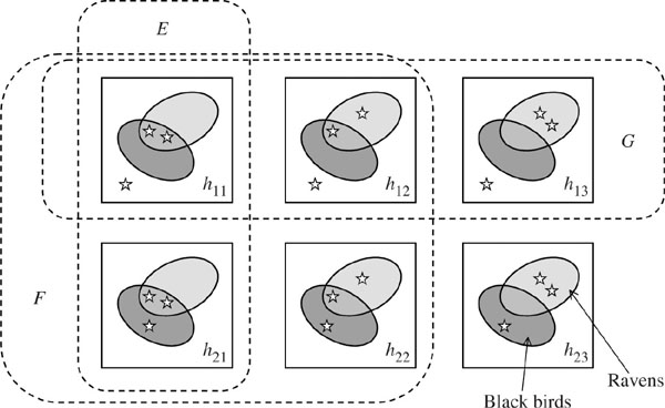
Figure 5.1. Hempel’s paradox. The stars represent three birds. Two of the birds are ravens and the other isn’t. Each square represents a possible state of the world labeled with its probability before any observation is made. The event E corresponds to the claim that all ravens are black. After observing a black raven, we learn that the event F has occurred. After observing a pink flamingo, we learn that the event G has occurred. What are prob(E|F) and prob(E|G)?

5.5.1 Justifying the Formula?

The confusion commonly engendered by Hempel’s paradox and our vulnerability to the base-rate fallacy suggests that we ought to think hard about Kolmogorov’s definition of a conditional probability when we seek to make use of his abstract mathematical theory in a particular context.

It is easy to justify Kolmogorov’s definition in the objective case when probability is to be interpreted as a naturally occurring frequency, like the rate at which uranium atoms decay. It is harder to justify the definition in the subjective case when probability is interpreted in terms of the odds at which someone is willing to bet on various events. It is still harder to find reasons why one should use Kolmogorov’s definition in the logical case when probability is to be interpreted as the rational degree of belief given the available evidence.

These interpretive issues are discussed at length in later chapters, but it is important at this stage to emphasize that the Kolmogorov theory itself offers no source of authority to those who advocate one interpretation of probability as opposed to another. The predictive success of the theory in physics certainly provides immense empirical support for the frequency interpretation where this applies, but one can’t parlay this into support for the aptness of Kolmogorov’s definition of a conditional probability when probability isn’t interpreted as a frequency.

Since Bayes’ rule is deduced from Kolmogorov’s definition of a conditional probability by a trivial algebraic manipulation, the same goes for Bayesian updating too. It isn’t written into the fabric of the universe that Bayes’ rule is the one-and-only correct way to update our beliefs. The naive kind of Bayesianism in which this assumption isn’t even questioned lacks any kind of foundation at all. A definition is just a definition and nothing more.

5.5.2 Independence

As in the case of conditional probability, Kolmogorov’s approach to independence is simply to offer a definition. Two events E and F are defined to be independent if the probability that they will both occur is the product of their probabilities. It then follows that

prob(E|F) = prob(E),

which is interpreted as meaning that learning F tells you nothing new about E.

Hempel’s paradox provides an example. We are surprised by Hempel’s argument because we think that the color of ravens is independent of the color of other birds. If we write this requirement into the model of figure 5.1, then h_ij = p_i × q_j and so

In this situation, sighting a pink flamingo therefore has no effect on the probability that all ravens are black.¹¹

5.5.3 Updating on Zero-Probability Events

Since we are never allowed to divide by zero, the definition (5.4) for a conditional probability is meaningless when prob(F) = 0. In 1889, Joseph Bertrand (1889) offered some paradoxes that illustrate how one can be led astray by failing to notice that one is conditioning on an event with probability zero. The versions given here concern the problem of finding the probability that a randomly chosen chord to a circle is longer than its radius.

One might first argue that the midpoint of a randomly chosen chord is equally likely to lie on any radius and that we therefore might as well confine our attention to one particular radius. Given that the midpoint of the chord lies on this radius, one might then argue that it is equally likely to be located at any point on the radius. With this set of assumptions one is led to the conclusion that the required probability is (section 10.3). On the other hand, if one assumes that the midpoint of the chord is equally likely to be anywhere within the circle, then one is led to the conclusion that the required probability is (section 10.3). Alternatively, we could assume that one endpoint of the chord is equally likely to be anywhere on the circumference of the circle, and that the second endpoint is equally likely to be anywhere else on the circumference, given that the first endpoint has been chosen. The required probability is then (section 10.3).

In such cases, Kolmogorov (1950) pragmatically recommends considering a sequence of events F_n with prob(F_n) > 0 that converges on F. One can then seek to define prob(E|F) as the limit of prob(E|F_n). However, different answers can be obtained by considering different sequences of events F_n. In geometrical examples, it is easy to deceive oneself into thinking that there is a “right” sequence, but we can easily program a computer to generate any of our three answers by randomizing according to any of our three recipes. For example, to generate a probability of approximately 0.87, first break the circumference of the circle down into a large number of equally likely pixels. Whichever pixel is chosen determines a radius that can also be broken down into a large number of equally likely pixels, each of which can be regarded as the midpoint of an appropriate chord.

One may think that such considerations resemble the cogitations of medieval schoolmen on the number of angels that can dance on the point of a pin, but one can’t escape conditioning on zero-probability events in game theory. Why doesn’t Alice take Bob’s queen? Because the result of her taking his queen is that he would checkmate her on his next move. Alice’s decision not to take Bob’s queen is therefore based on her conditioning on a counterfactual event—an event that won’t happen. I believe that the failure of game theorists to find uncontroversial refinements of Nash equilibrium can largely be traced to their treating the modeling of counterfactuals in the same way that one is tempted to treat the notion of random choice in Kolmogorov’s geometrical examples. There isn’t some uniquely correct way of modeling counterfactuals. One must expand the set of assumptions one is making in order to find a framework within which counterfactual conditionals can sensibly be analyzed (Binmore 2007b, chapter 14).

5.6 Upper and Lower Probabilities

Upper and lower probabilities can’t properly be said to be classical, but it is natural to introduce some of the ideas here because they are usually studied axiomatically. A whole book wouldn’t be enough to cover all the approaches that have been proposed, so I shall be looking at just a small sample.¹²

In most accounts, upper and lower probabilities arise when Pandora doesn’t know what probability to attach to an event, or doesn’t believe that it is meaningful to say that the event has a probability at all. I separate these two possibilities into the case of ambiguity and the case of uncertainty, although we shall find that the two cases are sometimes dual versions of the same theory (section 6.4.3).

5.6.1 Inner and Outer Measure

After the Banach–Tarski paradox, it won’t be surprising that we can’t say much about nonmeasurable events in Kolmogorov’s theory. But it is possible to assign an upper probability and a lower probability to any nonmeasurable event E by identifying these quantities with the outer and inner measure of E calculated from a given probability measure p.

We already saw how this is done in section 5.2.1 when discussing Lebesgue measure. The upper and lower probabilities will correspond to the outer and inner measures and m defined by (5.1) and (5.2) when the collection C consists of all measurable sets.

In brief, the upper probability of E is taken to be the largest number that is no larger than the probabilities of all measurable sets that contain E. The lower probability of E is taken to be the smallest number no smaller than the probabilities of all measurable sets that are contained in E.¹³ Since an event E is measurable in Kolmogorov’s theory if and only if its upper and lower probabilities are equal, we have that

whenever E is measurable and so p(E) is meaningful.

Hausdorff’s paradox of the sphere provides a good example. If we identify the sphere with the surface of Mars, we can ask with what probability a meteor will fall on one of Hausdorff’s three sets. But we won’t get an answer if we model probability as Lebesgue measure on the sphere, because each of Hausdorff’s sets then has a lower probability of zero and an upper probability of one (section 10.2).

Some examples of other researchers who take the line outlined here are Irving (Jack) Good (1983), Joe Halpern and Ron Fagin (1992), and Patrick Suppes (1974). John Sutton (2006) offers a particularly interesting application to economic questions.

5.6.2 Ambiguity

The use of ambiguity as an alternative or a substitute for uncertainty seems to originate with Daniel Ellsberg (1961), who made a number of important contributions to decision theory before he heroically blew the whistle on Richard Nixon’s cynical attitude to the loss of American lives in the Vietnam War by leaking what became known as the Pentagon papers. The Ellsberg paradox remains a hot research topic nearly fifty years after he first proposed it.

The Ellsberg paradox. Figure 5.2 explains the paradox. There is no way of assigning probabilities to the three possible events that is consistent with the choices most people make.

The standard explanation is that the choices people make reflect an aversion to ambiguity. They know there is a probability that a black ball will be chosen, but this probability might be anything between 0 and . When they choose J over K, they reveal a preference for winning with a probability that is certain to be rather than winning with a probability that might be anything in the range [0, ]. When they choose L over M, they reveal a preference for winning with a certain probability of to winning with a probability that might be anything in the range [, 1].

Bayesianism holds that rational folk are able to attach subjective probabilities to all events. Even if they only know that the frequency with which a black or a white ball will be chosen lies in a particular interval, they are still somehow able to attach a probability to each possible frequency. The behavior of laboratory subjects faced with the Ellsberg paradox is therefore dismissed as irrational. But I agree with David Schmeidler, who reportedly began his influential work on non-Bayesian decision theory with the observation that he saw nothing irrational in his preferring to settle issues by tossing a coin known to be fair, rather than tossing a coin about which nothing is known at all (see Gilboa and Schmeidler 2001).

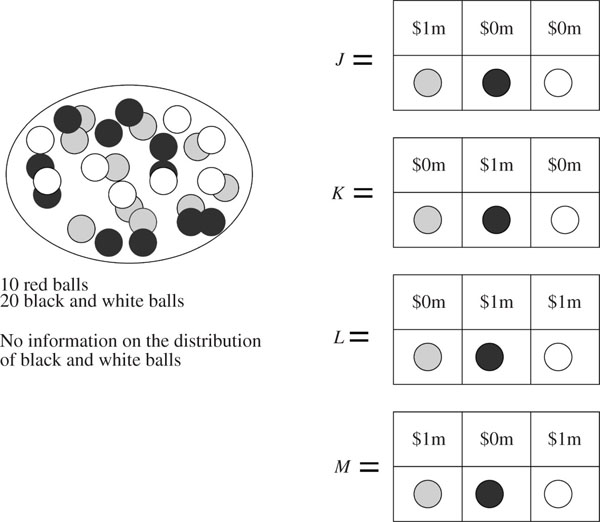
Figure 5.2. Ellsberg paradox. A ball is drawn from an urn containing ten red balls and twenty black or white balls. No further information is available on how many balls are black or white. The acts J, K, L, and M represent various reward schedules depending on the color of the ball that is drawn. Most laboratory subjects choose J rather than K and L rather than M. However, if the probabilities of picking a red, black, or white ball are respectively p, q, and r, then the first choice implies that p > q and the second choice implies that q > p.

5.6.3 Intervals of Probabilities

Ellsberg’s paradox makes it natural to think in terms of making decisions when the states of the world don’t come equipped with unambiguous probabilities, as in the Von Neumann and Morgenstern theory. What happens if we only know that the probability of a state lies in some range?

Quasi-Bayesian decision theory. One approach is to see what can be rescued from the Von Neumann and Morgenstern theory without adding any extra postulates. Giron and Rios (1980) undertook this task on the assumption that the class of probability measures that Pandora thinks possible is always convex. That is to say, if she thinks two probability measures over the set of states are possible, then she thinks that any probabilistic mixture of the two measures is also possible. The probabilities attached to any particular event will then lie in an interval.

If Pandora chooses a rather than b only when the expected utility of the act a exceeds that of b for all the probability measures she thinks possible, then we are led to an incomplete preference relation over the set of all her acts. In some cases, her criterion will leave the question of whether a or b should be chosen undecided.

In the spirit of revealed-preference theory, one can then seek to reverse the logic by asking what consistency postulates on an incomplete choice function ensure that Pandora will choose as though operating Giron and Rios’s quasi-Bayesian theory. However, I shan’t pursue this branch of revealed-preference theory any further. Walley (1991) is a good reference for the details.

The maximin criterion again. We really need a theory in which Pandora’s choices reveal a complete preference relation over the set of acts. One approach is to follow up a suggestion that originates in the work of Abraham Wald (1950)—the founder of statistical decision theory—who proposed a more palatable version of the maximin criterion of section 3.7.

When all that we can say about the possible probability measures over a state space is that they lie in a convex set, Pandora might first work out the expected Von Neumann and Morgenstern utility of all lotteries L(p) for each probability measure p that she regards as possible. She can then compute as the largest number no larger than each for all possible probability measures p. She can also compute as the smallest number no smaller than each for all possible probability measures p. However, only the lower expectation is treated as relevant in this approach, since the suggestion is that Pandora should choose whichever feasible action maximizes .

It can sometimes be confusing that the literature on statistical decision theory seldom talks about maximizing utility functions but expresses everything in terms of minimizing loss functions. What economists call the maximin criterion then becomes the minimax criterion. However, translating Walley’s (1991) work on what he calls previsions into the language of economics, we find that lower expectations always satisfy

where x and y are vectors of Von Neumann and Morgenstern utilities in which Pandora gets x_n or y_n with probability p_n, the vector e satisfies e_n = 1 (n = 1, 2, . . .), and . We shall meet these conditions again, but the immediate point is that if Pandora were observed making choices as though maximizing a utility function with these properties, than we could deduce that she is behaving as though applying the maximin criterion in the presence of a convex set of possible probability measures.

The (finite) superadditivity of (5.7) is always a straightforward consequence of taking the minimum (or infimum) of any additive quantity. One similarly always obtains (finite) subadditivity by taking the maximum (or supremum) of any additive quantity. The condition (5.8) that I have clumsily called affine homogeneity follows straightforwardly from the linear properties of expectations.

Gilboa and Schmeidler (2004) go much deeper into these questions, but, as with quasi-Bayesian decision theory, I shan’t pursue this line any further.

Nonadditive probabilities? There is another raft of proposals in which upper and lower probabilities are defined directly from a convex set of probability measures in much the same way as upper and lower expectations are defined from orthodox expected utility.

The upper probability of an event E is taken to be the smallest number that is no smaller than all possible probabilities for E. The lower probability of E is taken to be the largest number no larger than all possible probabilities for E. The difference between these concepts and the outer and inner measures of section 5.6.1 is that the problem is no longer that we may have no way to assign E any probability at all, but that we may now have many ways of assigning a probability to E.

Lower probabilities defined in this way have the following properties:

1. For any E, with equality for the impossible event E = Ø.

2. For any E, with equality for the certain event E = B.

3. If E and F have no state in common, then

The finite superadditivity asserted in (5.9) could be replaced by countable superadditivity when the probabilities from which lower probabilities are deduced correspond to (countably additive) measures, but only finite additivity can be asserted when the probabilities from which they are deduced correspond to (finitely additive) charges.

Upper probabilities have the same properties as lower probabilities, except that superadditivity is replaced by subadditivity. To see why, note that

where ~E is the complement of E (which is the set of all states in B not in E).

Set functions that satisfy properties additional to the three given above for are sometimes proposed as nonadditive substitutes for probabilities. David Schmeidler (2004) is a leading exponent of this school. One reason for seeking such a strengthening is that the three properties alone are not enough to imply that is a lower probability corresponding to some convex set of possible probabilities. Imposing the following supermodularity condition (also called 2-monotonicity or convexity) on an abstract lower probability closes this gap. Whether the events E and F overlap or not, we require that:

Schmeidler defends supermodularity as an expression of ambiguity aversion, but other authors have alternative suggestions (Gilboa 2004).

This discussion of nonadditive probabilities only scratches the surface of an enormous literature in which the notion of a Choquet integral is prominent. However, I shall say no more on the subject, since my own theory takes me off in a different direction.

¹ The spoof letters between Pascal and Fermat written by Alfréd Rényi (1977) are more entertaining than the real ones. Rényi’s potted history of the early days of probability is also instructive.

² American roulette wheels have a slot labeled 00, so they are more unfair than European wheels, since you are still only paid as though the probability of any particular slot coming up is 1/36.

³ There can only be a countable number of arcs in the collection, because each arc must contain a distinct point that makes a rational angle with a fixed radius. But there are only a countable number of rational numbers (section 1.7).

⁴ The full answer is that any Lebesgue measurable set is such a Borel set after removing a set of measure zero.

⁵ An acute angle lies between 0° and 180° inclusive.

⁶ If we are also willing to postulate the existence of “inaccessible cardinals.”

⁷ Formally, a probability space is a triple (B, , p), where B is a sample space, is a collection of measurable sets in B, and p is a probability measure defined on . Mathematicians express Kolmogorov’s measurability requirements by saying that must be a σ-algebra.

⁸ Nicholas Bingham (2005) provides an excellent historical survey of the views of mathematicians on finite additivity.

⁹ One only need consider sequences of sets that get larger and larger. Their limit can then be identified with their union.

¹⁰ If and 0 < prob(F) < 1, then it follows from the definition of a conditional probability that prob(E|F) > prob(E).

¹¹ In this analysis, p₁ is the probability that the bird which isn’t a raven isn’t black, and p₂ is the probability that it is. The probability that both ravens are black is q₁ = h₁₁ + h₂₁, the probability that one raven is black is q₂, and the probability that no ravens are black is q₃.

¹² Some references are Berger (1985), Breese and Fertig (1991), Chrisman (1995), DeGroot (1978), Dempster (1967), Earman (1992), Fertig and Breese (1990), Fine (1973, 1988), Fishburn (1970, 1982), Gardenfors and Sahlin (1982), Ghirardato and Marinacci (2002), Gilboa (2004), Giron and Rios (1980), Good (1983), Halpern and Fagin (1992), Huber (1980), Kyburg (1987), Levi (1980, 1986), Montesano and Giovannoni (1991), Pearl (1988), Seidenfeld (1993), Shafer (1976), Wakker (1989), Walley and Fine (1982), and Walley (1991).

¹³ If F stands for a measurable set, then