6

Frequency

6.1 Interpreting Classical Probability

Kolmogorov’s classical theory of probability is entirely mathematical, and so says nothing whatever about the world. To apply the theory, we need to find an interpretation of the objects that appear in the theory that is consistent with whatever facts we are treating as given in whatever model of the world we choose to maintain.

The literature recognizes three major interpretations of probability:

• Objective probability

• Subjective probability

• Logical probability

Donald Gillies’s (2000) excellent book Philosophical Theories of Probability surveys the literature very thoroughly from a perspective close to mine, and so I need only sketch the different interpretations.

Objective probability. We assume that probabilities are objective when making decisions under risk (section 3.1).

Theories of objective probability assume the existence of physical entities that generate sequences of outcomes about which one can say nothing useful beyond recording the frequency with which each outcome occurs in a very large number of trials. The length of time before a uranium atom decays is a good example.

Roulette wheels are an artificial device for generating the long sequences of trials that are necessary to make objective probabilities meaningful. I am particularly interested in such artificial randomizing devices, because they are needed in game theory to implement mixed strategies.

Subjective probability. We appeal to the theory of subjective probability when making decisions under uncertainty, although the circumstances under which this is legitimate remain controversial (section 3.1).

The subjective approach originates with the work of Frank Ramsey (1931) and Bruno de Finetti (1937). They invented what might be called a theory of revealed belief, in which Pandora’s beliefs are deduced from her behavior—just as her preferences are deduced from her behavior in the later theory of revealed preference.

If Pandora’s betting behavior satisfies certain consistency requirements, the theory of subjective probability argues that she will act as though she believes that each state of the world in B has a probability. These probabilities are said to be subjective, because Pandora’s beliefs may be based on little or no objective data, and so there is no particular reason why Quentin’s subjective probabilities should be the same as Pandora’s.

The theory of subjective probability is generally thought to have been brought to a state of perfection in Leonard (Jimmie) Savage’s (1951) much admired Foundations of Statistics. Chapter 7 describes how he succeeded in melding the ideas of Ramsey and de Finetti with those of Von Neumann and Morgenstern (section 7.2).

Bayes’ rule figures large in applications of the theory of subjective probability. Suppose, for example, that Pandora is observing the play at a roulette table. If she assigns each possible probability measure over the 37 numbers a positive prior probability, then Bayesian updating will always result in her subjective probabilities converging on the objective probabilities associated with the roulette wheel.¹

The emphasis on Bayes’ rule seems excessive to classical statisticians. It was presumably for this reason that Ronald Fisher dismissively referred to Savage’s synthesis as Bayesian decision theory. But the name stuck, and so people like me who see no problem in applying Savage’s theory to the small worlds in which he intended it to be used can nowadays be called Bayesians without any pejorative overtones.

Logical probability. A logical or epistemic probability for a proposition is the rational degree of belief it derives from the available evidence. Some authors speak instead of the credence or level of credibility of the proposition.

The logical interpretation of probability is the most difficult of the three considered in this book, but Rudolf Carnap (1950) and Karl Popper (1963) nevertheless thought it worthwhile to devote time to exploring its possibilities. The young John Maynard Keynes (1921) sought to establish his intellectual reputation with a book on the subject, but he was only the first of many who have found the project too ambitious. I think we are still so far from coming up with an adequate theory that I shall make no attempt to say anything systematic on the subject.

Not everyone agrees with this assessment. The prevailing orthodoxy in economics is Bayesianism, which I take to be the philosophical position that Bayesian decision theory always applies to all decision problems. In particular, it proceeds as though the subjective probabilities of Savage’s theory can be reinterpreted as logical probabilities without any hassle. So its adherents are committed—whether they know it or not—to the claim that Bayes’ rule solves the problem of scientific induction.

Outside economics, this kind of mindless Bayesianism is not so entrenched. One is faced instead with a spectrum of shades of opinion. I don’t suppose it is really possible to identify all the 46,656 different kinds of Bayesian decision theory that Jack Good claimed to identify, but there is certainly a whole range of views between the painfully naive form of Bayesianism common in economics and the bare-bones version of Bayesian decision theory that I defend in this book.

Let a thousand flowers bloom? Which is the right interpretation of probability? Fisher was firmly of the opinion that only objective probability makes sense. De Finetti was equally determined that only subjective probability is meaningful.

I subscribe to Carnap’s (1937) principle of tolerance. To insist either that there is a uniquely correct way to write a formal model of a particular intuitive concept or that there is a uniquely correct way to interpret a formal mathematical model is to venture into metaphysics. All three interpretations of probability therefore seem to me worthy of exploration. However, my own development of these interpretations doesn’t treat them as conceptually independent.

I think the three interpretations are more usefully seen as a system of expanding circles in which, for example, the randomizing devices that generate the data which determine objective probabilities are regarded as entities within the world in which Pandora makes the judgments that determine her subjective probabilities. Subjectivists may find it tiresome that adopting this point of view necessitates some hard thinking about Richard von Mises’ theory of randomizing devices, but that is the topic to which this chapter is devoted.

6.2 Randomizing Devices

Why do we need a theory of randomizing devices? In the case of a roulette wheel, for example, isn’t it enough to follow the early probabilists by simply assuming that each number is equally likely? In the case of a uranium atom, why not simply assume that it is equally likely to decay in any fixed time period, given that it hasn’t decayed already? There is a shallow answer, and what I regard as a deeper answer.

Osselots. When visiting India, I was taken to a palace of the Grand Mogul to see the giant marble board on which Akbar the Great played Parcheesi (Ludo) using beautiful maidens as pieces. Instead of dice, he threw six cowrie shells. If all six shells landed with their open parts upward, one could move a piece 25 squares—hence parcheesi, which is derived from the Hindi word for 25.

The Romans and Greeks liked to gamble too. Dice were not unknown, but the standard randomizing device was the osselot, which is the knee bone or heel bone of a sheep or goat. An osselot has six faces like a dice, but two of these are rounded, and so only four outcomes are possible when an osselot is thrown. Four osselots were usually thrown together. The venus throw required all four osselots to show a differently labeled face.

No two osselots are the same. The propensity of producing any particular outcome will therefore differ between osselots. Alfréd Rényi (1977) reports an experiment in which he threw an osselot one thousand times. The relative frequencies of each of the four faces were 0.408, 0.396, 0.091, and 0.105. A statistician would now be happy to estimate the probability of coming up with a venus in four independent throws of Rényi’s osselot as 24 times the product of these four relative frequencies (24 is the number of ways that four different faces can arise in four throws). The answer is 0.0371, which explains why the ancients used the throw of a venus as the exemplar of an unlikely event.

The point of this excursion into ancient gambling practices is that one can’t say anything accurate about the propensity of a particular osselot to fall on one of its faces without carrying out an experiment. It is true that, given a new osselot, one can appeal to experiments carried out on other osselots. For example, when estimating the probability of throwing a venus in the previous paragraph, it was assumed that Rényi’s osselot was typical of ancient osselots. But who knows what conventions governed the choice of the osselots in ancient Rome? What were the regional variations? How well could an expert estimate the probability of a face on a new osselot simply by examining it very closely? By how much has selective breeding changed domestic sheep and goats over two thousand years? Contemplating such imponderables makes it clear that 0.0371 can’t be treated as an objective estimate of the probability of throwing a venus in ancient times.

The necessity of doing empirical work with a particular osselot is plain, but the same is true of dice or roulette wheels if we are looking for real accuracy. It is true that modern dice are much more alike than osselots, but no two dice are exactly the same. Modeling dice as fair is therefore an idealization that is only justified up to a certain degree of accuracy. A million-dollar gambling scam in 2004 at London’s Ritz Casino illustrates the point. Bets could be placed after the roulette wheel was spun, but it turns out that one can do much better than guess that the outcome will be random if one comes equipped with a modern computer and a laser scanner that observes how and when the croupier throws the ball onto the wheel.

Philosophers of the skeptical school will go further and even ask how we know that a pair of perfectly symmetric dice will roll snake eyes (two 1s) with probability . Is it a synthetic a priori that a single perfectly symmetric dice will roll 1 with probability ?² Is it similarly a synthetic a priori that two dice rolled together are independent? When we ask the second question, are we saying that neither dice has any systematic effect on the other? If so, how are such considerations of cause and effect linked to Kolmogorov’s definition of independence?

The purpose of all this questioning is to make it clear that David Hume (1975) had good reason to argue that our knowledge of all such matters is based only on experience. If a work of philosophy tries to convince us of something, Hume suggests that we ask ourselves two questions. Does it say something about the logical consequences of the way we define words or symbols? Does it say something that has been learned from actually observing the way the world works? If not, we are to commit it to the flames, for it can contain nothing but sophistry and illusion.

The Vienna circle took this advice to an extreme that modern empiricists now largely disavow. It was thought, for example, that all definitions must be operational—that one can’t meaningfully postulate entities or relationships that aren’t directly verifiable by experiment. Nowadays, it is more usual to argue that a theory stands or falls on the extent to which its testable predictions are verified, whether or not all the propositions of the theory from which the predictions are deduced are directly testable themselves. This is the position I take in seeking to refine Richard von Mises’ theory, although he himself seems to have subscribed to the less relaxed philosophical prejudices of his time. However, von Mises’ insistence that objective probability must be based in principle on experimental data remains the foundation of the approach.

Living in sin? Von Neumann apparently said that anyone who attempts to generate random numbers by deterministic means is living in a state of sin. In spite of the random number generators that inhabit our computers and the success of internet casinos advertising randomizing algorithms that successfully mimic real roulette wheels, this attitude still persists. Traditionalists reject all algorithmic substitutes for a roulette wheel on the grounds that only physical randomizing devices can generate numbers that are “truly” random. But what does random mean? What tests should we apply to tell whether a device is random or not?

Kolmogorov (1968) was not a traditionalist in this regard. He was even willing to suggest a definition of what it means to say that a finite sequence of heads and tails is random. In recent years, the idea of algorithmic randomness has been developed much further by Greg Chaitin (2001) and others. To paraphrase Cristian Calude (1998), this computational school seeks to make precise the idea that an algorithmically generated random sequence will fail all effective pattern-detecting tests. Randomness is therefore essentially identified with unpredictability.

This idea is important to me because of its implications in game theory. Suppose, for example, that Alice is to play Bob at Matching Pennies (figure 9.5). In this game, Alice and Bob each show a coin. Alice wins if both coins show the same face. Bob wins if they show different faces. Every child who has played Matching Pennies in the playground knows the solution. In a Nash equilibrium, Alice and Bob will each play heads and tails with equal probability. How is the randomizing done? The traditional answer is that you should toss your coin before showing it.

If Alice plays Bob at Matching Pennies one hundred times in a row, she might toss her coin one hundred times in advance of playing. But what if it always falls heads? After ten games, Bob might conjecture that she will always play heads. When his conjecture fails to be refuted after ten more games, he might then always play tails and so win all the time. Alice will then wish she had chosen her sequence of heads and tails to satisfy some criterion for randomness like Kolmogorov’s.

A traditionalist will reply that an implicit assumption in rational game theory is that it is common knowledge that each player is rational. Bob will therefore know for sure that Alice chose her sequence randomly, and so her past play offers no genuine information about her future play. But I think that a theory that isn’t stable in the face of small perturbations to its basic assumptions isn’t very useful for applied work.

For this reason, I think it interesting to seek to apply von Mises’ theory of objective probability not only to natural randomizing devices but also to the kind of artificial devices that Von Neumann jocularly described as sinful.

6.3 Richard von Mises

Richard von Mises was the younger brother of Ludwig von Mises, who is still honored as a leading member of the Austrian school of economics. However, Richard’s espousal of the logical positivism of the Vienna circle put him at the opposite end of the philosophical spectrum to his brother.

His professional career was in engineering, especially aerodynamics. He flew as a test pilot for the Austro-Hungarian army in the First World War, but when the Nazis came to power, his Jewish ancestry made it prudent for him to take up a position in Istanbul. Eventually he was appointed to an engineering chair at Harvard in 1944. As with Von Neumann, his contributions to decision theory were therefore something of a sideline for him.

6.3.1 Collectives

In von Mises’ (1957, p. 12) theory, a collective is a sequence of trials that differ only in certain prespecified attributes. For example, the throws of pairs of dice in a game of craps are a candidate for a collective in which the attribute of a single throw consists of the pips shown on the two dice in that throw. The peas grown by Gregor Mendel in his pioneering work on genetics are a candidate for a collective in which the attributes of a single pea are the seven traits to which he chose to pay attention.

The probability of a particular attribute of a single trial within a collective is defined to be the limiting value of its relative frequency as more and more trials are considered. For example, in the sequence of heads and tails

the attribute of being a head has probability because its sequence of relative frequencies as we consider more and more trials is

which converges to .

However, we wouldn’t say that the coin that generated the sequence (6.1) has a propensity of one half to generate a head at every trial. Rather, it has a propensity to generate a head for sure at even trials and a tail for sure at odd trials. But von Mises wants to say that the same probability is to apply to an attribute no matter where in the sequence the trial we are talking about occurs. He therefore insists that his collectives are random.

What does random mean? Von Mises says that a collective is random if its probability remains unchanged when we pass from the whole sequence to a certain class of subsequences. For example, the sequence (6.1) isn’t random because the probability of the collective changes when we pass from the whole sequence of trials to the subsequence of odd trials.

Which class of subsequences do we need to consider when asking whether a collective is random? We can’t consider all subsequences because the subsequence consisting of all heads will have probability one whatever the probability of the original sequence may be.

Von Mises (1957, p. 25) tells us that the question of whether or not a certain trial in the original sequence should be allowed to belong to the subsequence must be settled independently of the result of that trial or future trials. Nowadays we would say that the subsequence needs to be defined recursively in terms of the outcomes only of past trials. Following work by Abraham Wald (1938) and others, Alonzo Church (1940) confirmed that nearly all sequences are random in this sense.

6.3.2 Von Mises’ Assumptions

Von Mises makes two assumptions about collectives:

1. The frequencies of the attributes within a collective converge to fixed limits.

2. The trials within a collective are random, so it doesn’t matter which trial you choose to look at.

He argues at length that these assumptions should be regarded, like any other natural laws, as summarizing experimental data.

Gambling systems. Von Mises defends his assumptions with an evolutionary argument (section 1.6). He points out that Pandora could be exploited if she tried to implement a mixed strategy using a randomizing device that failed his requirements for a collective. The next section suggests that she should be more picky still, but von Mises’ argument will still apply.

Suppose that the mixed strategy Alice is seeking to implement in Matching Pennies calls for heads to be played with probability . She plays repeatedly using a device that generates heads and tails with an overall probability of . However, she neglects to pay attention to von Mises’ second requirement. The result is that her sequence of heads and tails incorporates a recursively defined subsequence in which the probability of heads is . If Bob identifies this subsequence, he will play tails for sure whenever the next term of the subsequence is due. Alice will therefore end up losing on this subsequence.

Dawid and Vovk (1999) survey a substantial literature that interprets probability theory in such game-theoretic terms, but since my ultimate aim is to solve some game-theoretic problems by extending the scope of probability theory, I am unable to appeal to this elegant work.

Von Mises himself draws an analogy with perpetual-motion machines in denying the possibility of a gambling system that can consistently beat the bank at Monte Carlo. He then offers the survival of the casino industry as evidence of the empirical validity of his two requirements for roulette wheels. The survival of the insurance industry is similarly evidence for the fact that “all men insured before reaching the age of forty after complete medical examination and with the normal premium” is a collective if, for example, we take the relevant attributes to be whether or not an insured man dies in his forty-first year.

In such examples, von Mises repeatedly insists that his notion of an objective probability is meaningful only within the context of a properly specified collective. The same will be true of my attempt to refine his theory in the next section.

6.3.3 Conditional Probability

Section 5.5.1 emphasizes that Kolmogorov’s definition of a conditional probability is no more than a definition. When textbooks offer a reason for using his definition, they nearly always take for granted that probabilities are to be interpreted as frequencies. Von Mises’ theory of objective probability allows this explanation to be expressed in formal terms.

We need two collectives. A set F of attributes pertaining to the second collective determines a subsequence of trials in the first collective—those trials in which the outcome of the corresponding trial in the second collective lies in the set F. We then regard this subsequence as a new collective. If E is a set of attributes pertaining to the first collective, von Mises defines the conditional probability prob(E|F) to be the limiting relative frequency of E in the new collective.

To see why Kolmogorov’s formula (6.2) follows, we return to the baserate fallacy of section 5.5. The set I is the event that someone in a given population has a particular disease. The set P is the event that a test for the disease has produced a positive result. The numbers shown in figure 6.1 are consistent with the maintained hypothesis that the test gets the answer wrong 1% of the time.

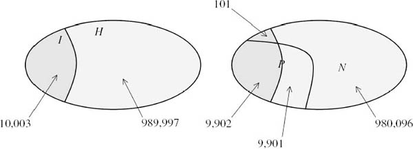
Figure 6.1. The base-rate fallacy. When laboratory subjects are given the actual numbers from an experiment, they make fewer mistakes (Gigerenzer 1996). The sample size in the figure is 1, 000, 000. The number of ill people is 10,003. The number of people who test positive and are ill is 9, 902. The number who test positive is 9, 902 + 9, 901. Thus #(P and I) = 9, 902, #(P) = 19, 803, and #(S) = 1, 000, 000. To realize that the probability of being ill having tested positive is about one half, one need only note that 9,902 is nearly equal to 9,901.

Nobody has any difficulty in seeing that the relative frequency with which people who tested positive are ill is

where #(S) is the number of people in the whole sample S, #(P and I) is the number of ill people who test positive, and #(P) is the number of people who test positive. If we let the sample size tend to infinity, the equation converges to

provided that the data conforms to von Mises’ requirements for a collective and prob(P) ≠ 0.

Independence. Von Mises’ theory also offers the following objective definition of what it means to say that two collectives are independent. If we confine our attention to a subsequence of one collective obtained by looking only at trials of which the outcome is a particular attribute of the second collective, then the probability of the subsequence must be the same as the probability of the original collective. That is to say, knowing the outcome of the second collective tells us nothing more than we already knew about the prospective outcome of the first collective.

Countable additivity? The objective probabilities defined by von Mises’ theory are finitely additive because the sum of two convergent sequences converges to the sum of their limits. However, as de Finetti (1974a, p. 124) gleefully pointed out, von Mises’ probabilities aren’t necessarily countably additive.

I don’t think that de Finetti was entitled to be so pleased, because it remains sensible to use countably additive models as simplifying approximations to objective probabilities in some contexts, just as it remains sensible to use continuous models in physics even though we now know that more can be explained in principle by treating space and time as though they were quantized (von Mises 1957, p. 37). On the other hand, de Finetti is right to insist that, within von Mises’ formal theory, we can’t hang on to countable additivity even if we allow the class of measurable sets to be very small—excluding perhaps all finite sets.

Consider, for example, the implications of defining the measure of a periodic set on the set of all integers to be its frequency. For each integer i, let P_i be a periodic set of integers with frequency that contains i. If we could extend our measure to be countably additive on some class of measurable sets, then the measure of would be less than the measure of the (countable) union of all P_i, which has been constructed to be no more than . But the measure of is 1.

6.4 Refining von Mises’ Theory

My own view of von Mises’ theory is that he is too ready to admit sequences as collectives. In particular, the relative frequency of an attribute of a collective should not simply converge on a limit p to be called its probability. The convergence should be uniform in a sense to be explained below.

6.4.1 Randomizing Boxes

In explaining why I think a new approach is useful, I shall stop talking about collectives and attributes to avoid confusion with von Mises’ original theory. Instead of a collective, I shall speak of a randomizing box whose name or label is an infinite sequence of real numbers belonging to an output set A. The label is to be interpreted as an idealized history of experimentation with a black box responsible for generating that output.

The output set A is the analogue of von Mises’ set of possible attributes. When the elements of the output set are probabilities, we can think of the randomizing box as an idealized implementation of a compound lottery. By reinterpreting heads and tails in such compound lotteries as and in Von Neumann and Morgenstern’s theory, we can think of randomizing boxes as acts among which Pandora may have preferences (section 9.2.1).

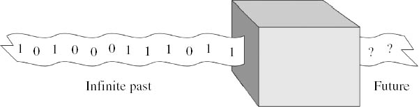
Figure 6.2. A randomizing box. The tape is to be envisaged as moving from right to left through the black box. When offered a new space, the box prints a 0 or a 1. It has printed an infinite sequence of such 0s and 1s in the past. This past history of the box serves as its label or name. What will be the next digit that emerges from the box?

In the simplest case, A = {0, 1} is the set consisting of only 0 and 1. The randomizing box is then a generalization of a coin-tossing device, with the fall of a head corresponding to the term 1 in the sequence and the fall of a tail corresponding to the term 0. Figure 6.2 represents this case as a traditional black box that has printed out an infinite sequence of 0s and 1s in the past, and the question is what we choose to say now about the next digit that it will print.

Skeptics argue that we waste our time trying to find an a priori reason why the next output of a randomizing box should be one thing rather than another. Didn’t David Hume teach us that we can’t even give an a priori reason to believe that the sun will rise tomorrow? However, the project here isn’t to find an a priori solution to the problem of scientific induction. As von Mises explained, the ultimate defense of his theory is experimental. Does it work in practice?

6.4.2 Uniform Convergence

When the attributes are heads and tails, von Mises requires of a collective that

where x_k = 1 if the kth trial is a head and x_k = 0 if it is a tail. The number p is then said to be the probability of heads within the collective.

This convergence requirement is to be compared with the outcome of a sequence of Bernoulli trials in which an unfair coin weighted to come down heads with probability p is tossed repeatedly. The strong law of large numbers then says that f_n → p as n → ∞ with probability one. It isn’t impossible that every trial might be a head (so that f_n → 1 as n → ∞), but the whole class of sequences that fail to satisfy (6.3) has probability zero.

An elementary proof of a version of the strong law of large numbers for the case when is to be found in Billingsley (1986, pp. 5–11). Following Émile Borel (1905), a real number x is first chosen from a uniform distribution on [0, 1]. The binary expansion of x is then taken to be the sequence of 0s and 1s whose limiting frequency is to be examined. A constructive argument is then given to show that the set of x for which (6.3) fails has Lebesgue measure zero.

This proof is easily adapted to show that the set of x for which

uniformly in m also has probability one.³ There is, of course, a sense in which this result must hold, since it would be very odd if throwing away a finite number of terms at the beginning of a sequence of independent trials could make a difference to limiting properties of the sequence that hold with probability one.

This fact seems a good reason for replacing von Mises’ requirement that f_n → p as n → ∞ by the requirement that f_n(m) → p as n → ∞ uniformly in m. The substitution has substantive consequences, but some mathematical preliminaries are necessary before they can be explained. A good reference for the mathematical details is Goffman and Pedrick (1965, pp. 62–68).

Extending linear functions. The set X of all bounded sequences x of real numbers is a vector space. In particular, given any two sequences x and y, the linear combination αx + βy is also a bounded sequence of real numbers. A subset Y of X that is similarly closed under linear combinations is a vector subspace of X. A linear function⁴ L : Y → always satisfies

L(αx + βy) = αL(x) + βL(y).

We can always extend a linear function L : Y → defined on a subspace Y to the whole of a vector space X. Given any z not in Y, the set Z of all x that can be written in the form y + γz is the smallest vector subspace of X that contains both Y and z. To extend L from Y to Z, take L(z) to be anything you fancy and then define L(x) for each x = y + γz in Z by

L(x) = L(y) + γL(z).

In this way, we can extend L step by step until it is defined on the whole set X.⁵

We can actually extend L from Y to X while hanging on to some of its properties. Suppose that λ : X → is (positively) homogeneous and (finitely) subadditive. This means that, for all α 0, and for all x and y,

1. λ(αx) = αλ(x);

2. λ(x + y) λ(x) + λ(y).

The famous (but not very difficult) Hahn–Banach theorem says that if L(y) λ(y) for all y in the subspace Y, then we can extend L as a linear function to the whole of X so that L(x) λ(x) for all x in X.

We noted one application in chapter 5. Lebesgue measure can be extended from the measurable sets on the circle as a finitely additive function defined on all sets on the circle. However, the application that we need in this chapter concerns the existence of Banach limits.

Extending probability? We now return to randomizing boxes in which the output set A consists of all real numbers in [0, 1]. Each such number will be interpreted as the probability of generating a head in a lottery that follows.

We are therefore talking about compound randomizing boxes that might implement the compound lotteries of section 3.4. However, in doing so we are getting ahead of ourselves, because we haven’t yet decided exactly what is to count as a randomizing box, nor whether such randomizing boxes will serve to implement the kind of lotteries we have considered in the past. In pursuing these questions, von Mises’ second requirement on randomness will be put aside for the moment so that we can focus on his first requirement. Why do I think this needs to be strengthened by appending a uniformity condition?

Suppose a randomizing box is labeled with a sequence x of real numbers x_n that represents its history of outputs. When can we reasonably attach a probability p(x) to this sequence that can be interpreted as the probability of finally ending up with a head on the next occasion that the randomizing agent offers us an output?

To be interpreted as a probability, we need the function p : X → from the vector space of all bounded sequences to the set of real numbers to satisfy certain properties. It must be linear, so that lotteries compound according to the regular laws of probability. We then insist on the following minimal requirements:

1. p(x) 0 when x_n 0 for all n = 1, 2, . . . ;

2. p(e) = 1 when e_n = 1 for all n = 1, 2, . . . ;

3. p(x) = p(y) when y is obtained by throwing away a finite number of terms from x.

It is easy to locate a linear function p that satisfies these requirements on some vector subspace of X. We need only set p(x) equal to the limit of any sequence x that lies in the subspace Y of convergent sequences. Is there an unambiguous way to extend p to a larger and more interesting subspace? Fortunately, this question was answered by a self-taught mathematical prodigy called Stefan Banach.

We can extend p from Y to the whole of X in many ways. Banach identified the smallest vector subspace Z on which all of these extensions agree. The sequences in the subspace Z are said to be “almost convergent.” The value of p(z) when z is an almost convergent sequence is called its Banach limit.

If the probability function p is to be extended unambiguously, we must therefore restrict it to the almost convergent sequences. This requirement entails appending our uniformity requirement (6.4) to von Mises’ assumption that the relative frequency of a sequence x should converge to p(x).

A finitely additive measure on the natural numbers. What intuition can be mustered for denying that a randomizing box necessarily has probability of generating a head, when its past history consists of a sequence y of heads and tails in which the relative frequency of heads converges to ? I think Banach teaches us that the distribution of the terms of y may be too wild for it to be meaningful to attach probabilities to its outputs. Von Mises’ theory therefore leaves us in an uncertain world rather than a risky world.

Waiting for a bus is a possible analogy. With the uniformity condition, Pandora is guaranteed that the frequency with which buses arrive will be close to the advertised rate, within a long enough but finite period. Without the uniformity condition, the bus frequency may balance out at infinity, but what good is that to anybody?

We can flesh out the bones of this intuition with the following construction. Given a set S of natural numbers, define a sequence x(S) by making its nth term equal to 1 if n belongs to S and 0 if it doesn’t. The function µ defined on certain subsets of the natural numbers by

is then finitely additive. Roughly speaking, the definition says that the number of elements of S in any interval of length can be made as close as we like to µ(S) by making sufficiently large.

Many authors would call µ a finitely additive measure, although it isn’t countably additive, and so it isn’t properly a measure at all. In section 5.3.1, we agreed that functions like µ would be called charges. The domain of µ can’t be all subsets of natural numbers, because p is only defined on sequences in Z. The sets on which µ is defined should perhaps be called chargeable, but I am going to call them measurable, although one can only count on finite unions of measurable sets being measurable when talking about charges.

The charge µ treats every natural number equally. We have seen that there is no point in looking for a proper measure that does the same (section 6.3). The best that can be said for µ in this regard is that it is countably superadditive.

Returning to a randomizing box that fails the uniformity test, we can now observe that the set of natural numbers corresponding to heads in the sequence y isn’t measurable according to µ. People who won’t wait for buses that arrive when y produces a head can therefore be regarded as uncertainty averse, because they don’t like events being nonmeasurable.

6.4.3 Objective Upper and Lower Probabilities?

What do we do when a randomizing box doesn’t have a probability? What action should Alice take, for example, if Bob deliberately uses such a randomizing box when choosing his strategies in a game they are playing together?

Within von Mises’ theory. Popper (1959) considered the possibility that the sequence f of relative frequencies given by (6.3) might not converge. His response was to draw attention to the cluster points of f, which he called “middle frequencies.”⁶ Walley and Fine (1982) explore this point of view in considerable detail.

A cluster point c has the property that we can find a subsequence of f that converges on c. As figure 6.3 indicates, the relative frequency f_n gets arbitrarily close to any cluster point c for an infinite number of values of n.

When x is a sequence of 0s and 1s, a Bayesian might hypothesize that a 1 occurs independently at each trial with probability p. If this were true, then updating by Bayes’ rule from a prior probability measure that attaches positive probability to both 0 and 1 generates a posterior probability measure that eventually puts all its weight on the correct value of p. But when we do the same with a sequence x for which the associated sequence f of relative frequencies doesn’t converge, then the posterior probability measure oscillates through all the cluster points of f, sometimes putting nearly all of its weight on one cluster point and sometimes on another.

This discussion suggests that a putative collective whose sequence of relative frequencies doesn’t converge might be treated as a problem in ambiguity, with the interval I of figure 6.3 taking on the role of the convex set of probability measures among which Pandora is unable to make a selection (section 5.6.3).⁷ The largest cluster point can then be taken to be the upper probability (x) of getting a head, and the smallest cluster point can be taken to be the lower probability (x). In mathematical notation:

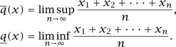
In the case when I contains only a single point because (x) = (x), the sequence x is a candidate for a von Mises collective because it satisfies his first requirement (6.3). Its von Mises probability q(x) is the common value of its upper and lower probabilities.

Refined upper and lower probabilities. For any > 0, we can find an N such that for any n > N

In fact, (x) and (x) are respectively the smallest and the largest numbers for which this assertion is true.

My theory of randomizing boxes requires that (6.6) be strengthened. For (x) and (x) to be upper and lower probabilities, we need them to be respectively the smallest and largest numbers for which the following uniformity condition holds.

For any > 0, we can find an N such that for any n > N

for all values of m.

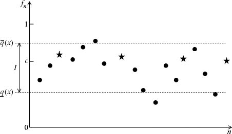
Figure 6.3. Cluster points. The figure shows a divergent sequence f of relative frequencies derived from a sequence x whose terms lie between 0 and 1. The starred terms of f are a subsequence that converges to the cluster point c. The interval is the set of all such cluster points.

Because (6.7) is a stronger condition than (6.6),

Notice that a sequence x may have and so have a probability in the sense of von Mises, but nevertheless not have a probability in the refined sense, because

Properties of upper and lower probabilities. Recall that x can be interpreted as a sequence of Von Neumann and Morgenstern utilities. It is therefore unsurprising that (x) behaves like a lower expectation (section 5.6.3):

where and e is the sequence whose terms are all 1.

Analogous properties for follow (with superadditivity replaced by subadditivity), because and so

Uncertainty. Section 5.6 briefly examined two ways of thinking about upper and lower probabilities. The first of these treated them as outer and inner measures (section 5.6.1).

Recall that (6.5) defines a charge (or finitely additive measure) on the set of natural numbers (section 6.4.2). For any set T of natural numbers, we construct a sequence x(T) whose nth term is 1 if n lies in T and 0 if it doesn’t. If the sequence x(T) has a probability p(x(T)) in our refined sense, we say that the set T is measurable (or chargeable) and that its charge is μ(T) = p(x(T)).

If S is nonmeasurable in this sense, we can define its inner charge (S) to be the largest number no larger than every µ(T) for which T is a measurable subset of S. Similarly, we can define its outer charge to be the smallest number no smaller than every µ(T) for which T is a measurable superset of S.

Do our definitions of and (S) accord with those of and (x(S))? In particular, is it true that = To see that the answer is yes, we need to return to (6.7).

We can approximate as closely as we like by the charge µ(T) of a measurable superset T of S. In the case when T is measurable, our definitions say that the number of elements of T in any interval of length can be made as close as we like to µ(T) × by making sufficiently large. Our problem in connecting this fact with the definition of is that (6.7) only tells us that the measurability requirement for the set S itself holds for an infinity of intervals of length , but not necessarily for all such intervals. However, we can replace 0s by 1s in the sequence x(S) until our new sequence x(T) satisfies the measurability requirement for all intervals. The resulting measurable superset T of S then supplies the necessary connection between and .

Ambiguity. In the refined version of von Mises’ theory, the uncertainty approach to upper and lower probabilities is mathematically dual to the ambiguity approach (section 5.6). There is therefore an important sense in which it doesn’t matter which approach we take. Personally, I find the ambiguity approach intuitively easier to handle.

The theory of Banach limits (section 6.4.2) depends heavily on the properties of and (x). Any Banach limit defined on the space of all bounded sequences is first shown to satisfy

So all Banach limits are equal when (x) = . It follows that there can be no ambiguity about how to define the probability p(x) that a randomizing box will generate a head when x is almost convergent (section 6.4.2). We have no choice but to take p(x) = (x) = .

But suppose that z isn’t almost convergent, so that (z) < . We can then extend p as a Banach limit from the space of almost convergent sequences so as to make p(z) anything we like in the range:

I = [(z), ].

Simply take the function λ in the Hahn–Banach theorem to be (x) (section 10.4).

This fact links my approach with the ideas on ambiguity briefly surveyed in section 5.6.3. If the set of all possible probability functions is identified with the set of all Banach limits, then (z) is the maximum of all possible probabilities p(z), and (z) is the minimum.

Alternative theories? Someone attached to von Mises’ original theory may reasonably ask why we shouldn’t append additional requirements to the three conditions for a Banach limit given in section 6.4.2, thereby characterizing what might be called a super Banach limit. The space on which such a super Banach limit is defined will be larger than the set of all almost convergent sequences, and so more sequences will be assigned a probability.

For example, we could ask that von Mises’ first requirement be satisfied, so that any x whose sequence of relative frequencies f converges to a limit p is assigned the value q(x) = p. The Hahn–Banach theorem with λ = can then be used to extend q to the set of all bounded sequences. The upper and lower probabilities of x would then be (x) and (x).⁸ But why not go further and require that p(x) = p whenever x is (C, k) summable to p? Why not allow some even wider class of summability methods for assigning a generalized limit to a divergent sequence (Hardy 1956)?

I don’t think that there is a one-and-only correct model. My refinement of von Mises’ theory is simply the version that carries the least baggage.

6.5 Totally Muddling Boxes

Von Mises second requirement is that a collective be random. Recall that his definition requires that a collective with probability q should have the property that every effectively determined subsequence should also have probability q.

If von Mises had permitted collectives with upper and lower probabilities and , he would presumably have asked that every effectively determined subsequence should also have upper and lower probabilities and .⁹ I don’t know whether Alonzo Church’s (1940) vindication of von Mises’ second requirement would extend to this case, but even if it did, it wouldn’t be of any direct help in dealing with the randomizing boxes introduced in section 6.4.1.

Randomizing boxes diverge from collectives not just in satisfying a uniformity requirement, but in being structured differently (section 6.4). A randomizing box isn’t envisaged as an ongoing process in which we seek to predict the probability that the next trial will be a head. The label x on a randomizing box is a full description of a countably infinite number of trials that have already been carried out.

Without changing anything that matters, one could therefore envisage the tape of figure 6.2 as being reversed, so that the first term of the sequence x lies infinitely far to the left of the box.¹⁰ The digit about to be printed then has no immediate predecessor. No algorithm that examines only a finite number of terms of x can therefore say anything relevant about the value of p(x), which depends only on the limiting properties of x. A randomizing requirement is therefore redundant.

This approach sweeps the randomness problem under the carpet by exploiting the fact that the label x of a randomizing box is idealized to be an infinite sequence. However, any attempt to produce a finite computer program that approximates the properties of a randomizing box wouldn’t be able to avoid ensuring that the next digit to be printed can’t ever be predicted in an appropriate sense by examining the digits already printed (Stecher and Dickhaut 2008).

Muddling boxes. A muddling box will be understood to be a randomizing box that offers Pandora no grounds for taking into account any of its properties other than the values of its upper and lower probabilities. For example, if it were meaningful to say that the terms of its sequence f of relative frequencies were only occasionally close to its lower probability, we would want to attach more importance to its upper probability. The weight we attached to the upper probability would then be an additional factor that would need to be taken into account when evaluating the randomizing box.

My suggestion for coping with this problem uses the explicit formulas:

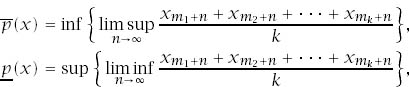
in which formulas the infimum and supremum range over all finite sets {m₁, m₂, . . . , m_k} of natural numbers (section 10.5).

In the case of the sequence x of (6.1) in which heads and tails alternate, we have that (x) = (x) = (counting a tail as 0 and a head as 1). However, taking k = 2, m₁ = 1, and m₂ = 3,

Looking at different sets {m₁, m₂, . . . , m_k} of natural numbers is therefore a way of eliciting the structure of a randomizing box.

The definition I propose for a muddling box is that for any > 0,

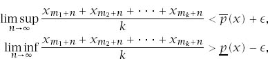
for all finite sets {m₁, m₂, . . . , m_k} of natural numbers whose cardinality k is sufficiently large. A totally muddling box is a muddling box for which (x) = 1 and (x) = 0.

¹ However, Diaconis and Freedman (1986) show that convergence on the true value of a parameter isn’t always guaranteed when the number of possible outcomes is infinite, even when the prior distribution is restricted in an attempt to eliminate the problem.

² Immanuel Kant (1998) claimed that some contingent facts about the world are known to us without our needing to consult our experience. His leading example of such a synthetic a priori was that space is Euclidean.

³ To say that f_n(m) → p as n → ∞ means that for any > 0 we can find N(m) such that |f_n (m) − p| < for any n > N(m). To say that f_n(m) → p as n → ∞ uniformly in m means that the same value of N will suffice in the definition of convergence for all values of m.

⁴ It is because we need to be precise about linearity at this stage that I was pedantic about calling affine functions affine in previous chapters.

⁵ To justify this claim, it is necessary to appeal to Zorn’s lemma (actually proved by Hausdorff) or some other principle that relies on the axiom of choice.

⁶ Cluster points are also called points of accumulation or limit points.

⁷ The set of cluster points of a sequence need not be convex in general, but if x is a bounded sequence, then the set of all cluster points of f is necessarily convex.

⁸ The argument of section 10.4 works equally well with p replaced by q.

⁹ Karl Popper (1959, appendix IV) offers an alternative to von Mises’ definition of randomness that allows for differing upper and lower probabilities, but it doesn’t seem adequate to me.

¹⁰ Thereby inverting Wittgenstein’s philosophical joke about the man he heard finishing a backward recital of the decimal expansion of π by saying . . . 95141.3.