Chapter 2

HOW TO DRAW A STRAIGHT LINE

The straight line is a stronger and more profound expression than the curve.

Piet Mondrian

 

 

This chapter heading comes from a book by A. B. Kempe, How to Draw a Straight Line: A Lecture on Linkages (Kempe 1877). The charm and gentle tone of the book suggest that the original lectures must have been a delightful experience. If you ask most people what a straight line is their answer will probably involve ‘the shortest distance between two points’. Of course they do not always mean this since the shortest distance to the Antipodes from Yorkshire is downwards through the centre of the Earth: these two places are at opposite ends of a diameter. What they probably mean is the arc of a path on the surface of the Earth which is a great circle. In this chapter we shall adopt the usual geometers’ convention and claim that the Earth is flat. By restricting ourselves in this way, we return to the usual idea of a straight line in a plane. The obvious way to draw such a straight line is to use a rule or straight edge but, of course, this argument is circular and Kempe (1877) makes much play of the need to make the ‘first’ straight line. More serious practical problems arise if the rule is simply not long enough or if it is needed not to guide a pen or pencil but a piece of heavy moving machinery. Here we focus the discussion on the application of linkages for this latter purpose although, to be true to the chapter heading, we include a section on how to make models of linkages that can be used to draw a straight line using a variety of techniques.

To appreciate fully the significance of linkages it is necessary to go back over 200 years to examine the development of steam power and, in particular, the beam engine, to see why these linkages played an essential part in the Industrial Revolution that led to the economic growth and prosperity of the United Kingdom in the eighteenth and nineteenth centuries.

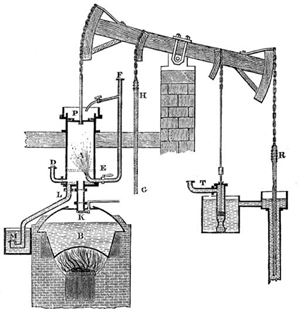
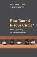
Figure 2.1. A chain used in beam engine transmission.

Figure 2.1 shows a very much simplified beam engine. The vertical cylinder, with its piston P and rod, transmits power to rock a beam at the other end of which there was commonly a long rod R driving a pump, typically to clear water from a mine. In very early beam engines, such as that shown, the steam in the cylinder condensed as the valve at E was opened to let in cold water. This created a vacuum in the cylinder and it was the force of atmospheric pressure that pushed the piston down. It was only later that the direct expansion of steam created the force which drove the piston.

In any case, the piston rod is designed only to take axial loads, that is to say a push or pull. Its generally slender form is not designed to resist sideways loading forces and so it must somehow be constrained to move in a straight line. However, the end of the beam to which it must be connected can only move in the arc of a circle. If the piston rod were connected directly to the beam then the piston rod would be subjected to sideways forces and the engine would rapidly wear out, assuming of course that it even worked in the first place.

To experience, literally first hand, some of the consequences of not sending the piston rod in a straight line take a cafetière and, to be on the safe side, fill it with cold water rather than hot coffee. If you can manage to depress the plunger carefully so as to keep contact between the rod and the hole in the lid to a minimum you have achieved the ideal: the rod has not been subjected to any lateral forces and the wear on it and the lid of the cafetière is at a minimum. Repeat the exercise, but this time do it more hurriedly: the rod will rub against the lid and often cause it to tip up or even come off the top completely. In extreme cases the whole body of the cafetière might tip and spill some of the contents. Now change some of the words in this paragraph; substituting ‘stuffing box’ for ‘hole in the lid’, ‘cylinder cover’ for ‘lid’, and ‘cylinder’ for ‘body of the cafetière’ and you have reproduced exactly what could happen in a beam engine. You will have demonstrated the need for some form of guidance for the piston rod. You will also have noticed that the diameter of the hole in the lid is slightly larger than the plunger rod. Aside from the fact that cafetières are mass-produced non-precision goods, this clearance, or play, illustrates an important aspect of design in all pivots: there must be some clearance, otherwise all joints would be too stiff to move and lubrication would be impossible. The significance of this apparently trite and obvious observation is that in any system of links there must inevitably be some play or tolerance in the movement of the pivot designed to provide the straight-line guide. This implies that the geometry of a linkage need not describe an exact straight line provided its theoretical departure from true linearity lies within the practical tolerances or play of the system to which it is being applied.

Incidentally, the need for straight-line linkages did not arise with beam engine design because the first engines were single acting: that is, power was developed only on the downstroke of the piston and the return upstroke was achieved by simply balancing the beam and pump to pull the piston up. When the piston was moving down it was pulling the beam, on the upstroke the roles were reversed and the beam pulled the piston. In this way the connection between the piston rod and the beam was always under tension and it was quite acceptable to use a chain; the end of the beam was in the form of a large circular arc, i.e. a sector (see figure 2.1). You can still see this mode of working in a ‘nodding donkey’, used for pumping oil from wells.

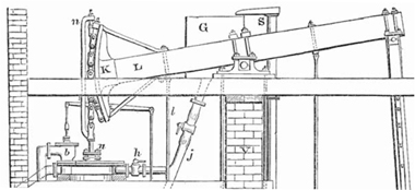
Figure 2.2. Francis Thompson’s opposed chains.

One of James Watt’s many innovations and improvements to engine design was to have double-acting engines. Power was then developed on both the upstroke and the downstroke and a chain connection between rod and beam was clearly no longer a possibility—you can pull a chain but you cannot push with it. One solution was to use two chains, and this option was taken by Francis Thompson in Ashover in around 1783. His atmospheric engine, part of which is shown in figure 2.2, had two separate and opposed cylinders. The two chains worked under tension in opposite directions.

Another solution was to fit teeth to the piston rod engaging with pegs on the beam. Neither of these solutions was entirely satisfactory, the additional chain increased the height of the engine and the rack was noisy. Workshop technology at that time, the 1780s, was not capable of producing long straight guides and although they could have been made in sections, their cost of manufacture and the cost of erection would have been so high that beam engines would have been totally uneconomic.

Figure 2.3. Teeth on the piston engaging with pegs on the beam.

This is a very brief introduction to the problem of producing straight-line guides to take advantage of the effectively doubled power output of double-acting steam engines. Although beam engines have long been superseded, the need for such linkages still exists in a variety of engineering applications, and linkages for other straight-line motions are part of everyday living. Look at the hinges on cars, modern windows and windscreen wipers. Rarely do they use simple hinges.

The original name for these was ‘parallel motion’ linkages for reasons that are not exactly clear, although this term was widely used as you will see if you ever look in an old book about steam power or mechanical engineering. No attempt is made here to try to describe the whole range of linkages that have been invented over the years, but rather we present a selection of the best known, practically important or geometrically most interesting. We have divided the linkages into three categories.

The first category is of approximate straight lines. Although the idea of an approximate straight line sits uneasily, as mentioned above it is often a perfectly acceptable solution to a real engineering problem. It should be emphasized that departures from a true straight line are inherent in the geometry of the linkage and not a consequence of either poor workmanship or deliberate play in the joints. In the second category of linkages the geometry is such that if they are correctly made they will generate an exact straight line.

The last category comprises guide linkages. These are hybrid linkages in the sense that they rely on one of their pivots being itself guided in a straight line. This may almost sound like cheating, but their importance is that they magnify this guided movement so that a part of one link moves in a straight line but over a much greater distance. It is much cheaper to make a short straight guide and use a linkage to increase its range than it is to machine a long guide.

2.1 Approximate-Straight-Line Linkages

James Watt (1736–1819) is remembered today for his pioneering work on steam engines, and his name is commemorated in the unit of power. His own view of his life’s work does not quite agree with current opinion: in old age he wrote to Matthew Boulton that

[a]lthough I am not over anxious after fame, yet I am more proud of the parallel motion than of any other invention I have ever made.

It was James Watt who invented the first straight-line linkage, and the idea of its genesis using links is contained in a letter he wrote to Boulton in June 1784.

I have got a glimpse of a method of causing a piston rod to move up and down perpendicularly by only fixing it to a piece of iron upon the beam, without chains or perpendicular guides ... and one of the most ingenious simple pieces of mechanics I have invented.

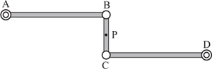
Figure 2.4. A schematic of Watt’s linkage.

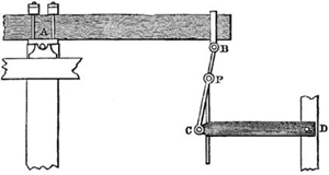
Figure 2.5. The general form of Watt’s linkage.

Watt published his linkage in a patent dated 24 August 1784, and it is important to remember that he did not claim it produced a true straight line. In a letter to Boulton on 11 September 1784 he describes the linkage as follows.

The convexities of the arches, lying in contrary directions, there is a certain point in the connecting-lever, which has very little sensible variation from a straight line.

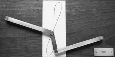
In its simplest form Watt’s linkage consists of just the following three bars, AB, BC and CD (see figure 2.4). Here A and D are fixed in space, but free to rotate, forcing B and C to move in arcs of circles, so that the two long arms AB and CD form the ‘arches’ to which Watt refers. Links AB and CD are the same length, and the centre of the short connecting link BC, labelled P, is the part that moves vertically in the approximate-straightline manner. It is worth noting that the length of AB does not have any particular relation to the length BC. Watt’s linkage also has a more general form with AB ≠ CD, illustrated in figure 2.5, in which P is positioned with the ratio

Figure 2.6. Watt’s linkage.

The longer the arms AB and CD are to BC, the better the path of P will approximate a straight line. Note that this result is only approximate, and only for small displacements of B, or equivalently C. The complete path taken by the point P is shown in figure 2.6.

Before going any further with Watt’s linkage we ought to look at the use of this linkage by Phineas Crowther (1763–1818). On paper it appears to be the same, and instead of drawing another figure, figure 2.6 showing Watt’s linkage is adequate. Crowther’s objective was to dispense with the beam by placing the crankshaft directly above the cylinder, the piston being constrained with a Watt-like linkage. The only real difference then is one of application: Watt’s was for beam engines whereas Crowther’s was constructed for conventional engines. He was an engineer from the northeast of England and the main application of his linkages was to winding engines, such as that shown in figure 2.7, made for hauling coal or ore wagons up inclines. We mention this because one of his working engines has been preserved and re-erected in the National Railway Museum in York and is routinely shown working, albeit with an electric drive, at frequent intervals throughout the day. According to Watkins (1953), such engines were popular and some were in continual use for decades.

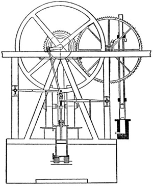
Figure 2.7. Crowther’s engine, from his patent (UK patent number 2378) of 1800.

The dimensions of this engine are known, so we use it as an example to show the movement of the piston rod, and in particular its departure from movement in a straight line. Since it is an old engine, the original imperial measurements have been used in the calculation. There is one slight difference from the Watt-type linkage shown in figure 2.4. At the centre of the stroke, when the arms AB and CD are horizontal, the centre link BC is not vertical but approximately = 5° from the vertical. The dimensions are as follows:

AB = CD = 132 in,

BC = 27 in, with P at the centre,

stroke   = 60 in.

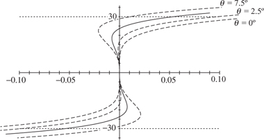
Figure 2.8. The path of the pivot in Crowther’s engine.

The horizontal distance between the fixed pivots at A and D is

2AB − BC sin (5°) ≈ 237.7in,

and the vertical separation is

BC cos (5°) ≈ 26.9in.

We can calculate the path taken by the point P as it travels through a complete stroke of 60 in, and this is shown in figure 2.8 with a solid line. We have repeated these calculations for values of ≠ 5° and included these using dashed lines for the purposes of comparison. Notice the vastly exaggerated horizontal scale of ± 0.1 units, compared with the vertical scale of ± 30 units. Hence, the path of P is actually quite a good approximation to a straight line, despite the appearance of figure 2.8.

What is clear is that the linkage is very sensitive to the positioning of the fixed pivots, and if the original 5° departure from vertical were to be rotated slightly, the departure of the path of P from a straight line would be greater at the ends of the stroke. Even so, the departure of ± 0.05 in at the ends of the stroke of 60 in, or 0.083%, is quite acceptable given the number of pivots and the amount of play in each.

The Crowther linkage is quite obvious on the engine, but on a beam engine it is sometimes difficult to distinguish the Watt linkage from the other parts. Furthermore, the beam is quite long and an arm of equal length would take up a prohibitive amount of space. To overcome this problem Watt developed the basic linkage into his ‘complete parallel motion’, also included in his original 1784 patent. While the original simple motion is rarely seen on beam engines, the complete parallel motion is much more common.

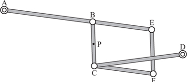
Figure 2.9. Watt’s complete parallel motion.

In the arrangement shown in figure 2.9 we have the main beam of the engine with its central pivot at A just as before. However, the point B is not at the end of the beam, which is E, but part way along. The rod CD, which is equal in length to AB and is known as the radius rod, is connected to the beam by a shorter link BC. The centre of this, P, will move in an approximate straight line. Here the link ABCD is exactly Watt’s or Crowther’s linkage as we had it before. The other links form a parallelogram BCEF, and the pivot F is connected to the piston rod. You are encouraged to consider the motion of F, which is of course critical. The most straightforward case is when the length AB equals that of BE, which is not the same as that illustrated in figure 2.9.

This figure also suggests why the term ‘parallel motion’ was used originally, because apart from having this more compact form, the two uprights in the parallelogram guide both the piston rod and the valve gears. An example of this is shown in figure 2.10. Here an extra vertical rod is attached to the driving rods of an air pump. Air in steam is a nuisance as it is not condensed and can therefore lead to a loss of power. Dickinson (1963) is a good starting point for more information about this and other practical aspects of steam engine history.

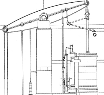
Figure 2.10. A beam engine with Watt’s linkage shown.

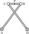
Figure 2.11. Chebyshev’s linkage.

Following Watt’s discovery a whole range of linkages was developed, and here we must limit the discussion to some of the more interesting. The first we consider was developed by the Russian mathematician Pafnuty Chebyshev (1821–94), who was fascinated by linkages. For many years he was of the firm belief that linkages could never be designed to produce exact straight lines. His best-known linkage is shown in figure 2.11.

In essence this consists of the three bars of Watt’s linkage with the radius arms crossed, but it is quite different in the strict requirement that the lengths of the links must be in the following proportions:

 

AD = 4,

AB = CD = 5,

CB = 2, with P at its centre.

In the mid position, as drawn, the linkage is symmetrical and the Pythagorean theorem can be used to show that P is 4 units above the baseline AD. When either of the linkages AB or CD is in the vertical position, P is again exactly 4 units above AB. It is well worth making a model of this linkage and looking at the complete path of P since there is an interesting curve between these positions. The complete curve traced is shown on the righthand side of plate 2, although you will immediately notice we have used a different linkage here. More on this in a moment.

For now notice that the curve appears to be made up of two parts, one of which appears to be straight, the other curved. The path of P does not actually follow a straight line, and figure 2.12 shows this part of the movement. Please note carefully that the vertical axis has been exaggerated wildly. The maximum deviation from the horizontal straight line y = 4 is less than 0.01 vertical units in a horizontal movement of 4 units, or 0.25%. Now, to put this departure from a true straight line in context, if we take the distance AD to be 100 mm, then the maximum departure from a straight line is 0.25 mm. Recall that we are forced to use broad lines in any sketch, and a common printed line width is around 0.2 mm. If you have a propelling pencil, this is likely to use graphite of 0.5 mm. If we draw the x- and y- axes on the same scale then the maximum theoretical deviation is about the same as the broad line used to draw it, so it will be hard to distinguish. We have tried to show this accurately in figure 2.12. The top is exaggerated and the bottom uses the same horizontal and vertical scales. Whether you can perceive a difference between the bottom two lines will depend to a large extent on the quality of the printing used to create this page!

There appears to be no connection between Chebyshev’s linkage and the arrangement of links shown in plate 2. However, we shall now show that the two arrangements produce identical curves, and we will show that the path of the second form can be calculated more easily and directly.

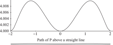
Figure 2.12. Chebyshev’s approximate straight line.

First draw Chebyshev’s linkage ABCD as before, as shown in the left-hand diagram of figure 2.13. Mark P as the midpoint of BC. Next draw a similar linkage A′B′C′D′ of half the size, with the same orientation, with D = D′, and with A′ on the line AD. Hence CP is parallel to B′C′ and these links are equal in length (one unit). Now draw a line through PB′ and extend this so the length equals CD. Then we have a parallelogram PCDE. In particular, as B and C move on a circle, with centre at P, E will move on a circle with a centre at D.

Conversely, if E moves on a circle of radius 1 with centre at D, then the three-bar linkage A′B′, PE, ED forces P to move along the midpoint of the line BC, where B and C are part of Chebyshev’s original linkage. Hence, if we construct an arrangement consisting only of DE, A′B′ and EP, we know that P will follow the path of Chebyshev’s original linkage. This is the alternative form shown in plate 2.

In the original form of the linkage the point P crosses over the two links AB and CD during one complete motion. In the second form the point P is unobstructed, and the motion of the linkage can be driven by a circular motion of E. Alternatively, the straightest part of the curve can be obtained by reciprocating the motion of E on a circular arc. Both of these aspects are significant practical considerations, making the second form much more useful. It is also easier to calculate the path of P from geometrical considerations in this second form, since we have that A′B′ = B′P′ = B′E.

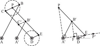
Figure 2.13. Chebyshev’s original and alternative linkages superimposed.

We begin our detailed examination of Chebyshev’s alternative linkage by providing a new diagram, without the original linkage in place. This is shown on the right-hand side of figure 2.13.

We recall that A′B′ = B′P′ = B′E. Furthermore, PA′E is a right-angled triangle with right angle at A′. If we drop a perpendicular from B′ onto A′E, and mark this point as F, then, by similar triangles,

So that

Extending the line A′E if necessary, mark P′ on A′E so that A′P = A′P′. We take the origin to be A′ and E to have coordinates (x, y), then P′ has coordinates

and by a direct transformation, P will have coordinates

By taking

E = (x, y) = (A′D + DE cos(s), DE sin (s)),

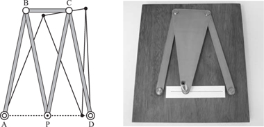
Figure 2.14. Roberts’s linkage.

and noting that (A′E)² = x² + y², we can put all the pieces together to obtain an explicit formula for the path P in terms only of the lengths of the links, and the angle s. As you can see, this does not result in a satisfying, simple formula. It is a great pity that mechanisms as simple as these linkages, in either original or more general forms, do not yield neat mathematical descriptions in elementary terms. Surprisingly there are many other arrangements of linkages which will also produce exactly this curve.

A further development was made by Richard Roberts (1789–1864). It is another example of a Watt-type linkage, and here the restrictions on link lengths can be relaxed. All that is necessary is that

AB = BP = CP = CD

and

BC = AD.

A model of Chebyshev’s crossed linkage can be modified by uncrossing the links and then adding an arm. An example is shown in figure 2.14, with an accompanying schematic.

The trace of P as it moves between A and D is a very close approximation to a straight line. For the purposes of comparison with Chebyshev’s straight line in figure 2.12 we take exactly the same linkages, supplemented with the extra bar in figure 2.14. Then, without details of the calculation, the path of P is shown in figure 2.15, showing a substantial improvement. Again, the vertical axis has been exaggerated wildly and the maximum deviation from the horizontal straight line y = 0 is less than 0.0022 vertical units in a horizontal movement of 4 units, or 0.06%.

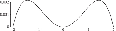
Figure 2.15. Roberts’s approximate straight line.

All these examples of Watt-type linkages involve two fixed points and three bars. In some sense the two fixed points lie on a fourth bar. Hence we refer to these as four-bar linkages. The free ends of the two fixed bars must move in circles, and so we consider a point P relative to the third bar. Notice the progression from a point P on the link between B and C, then on an extension arm in line with BC, and then in Roberts’s mechanism to an arbitrary point not on the line BC but in a position fixed relative to it. This is the most general situation possible without the addition of extra linkages.

2.2 Exact-Straight-Line Linkages

Historically, the first of these linkages was described by Pierre Frédéric Sarrus (1798–1861) in 1853. It differs from all the other linkages so far described in this chapter in that its parts move in three dimensions rather than just the two dimensions of planar linkages. Although it may not have been used in steam engines it is applied widely in jacks, elevating platforms and similar devices. The crude model in plate 3 shows that the pivots are more akin to hinges, making it look like a short section of a concertina. Although in its completed form it looks complex, the opened-out photograph shown illustrates how simple the mechanism is. A full description of Sarrus’s mechanism and other similar hinged systems is given in Dunkerley (1912).

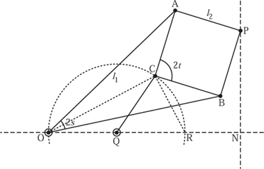
Figure 2.16. Peaucellier’s linkage.

The first planar linkage was invented by Charles Nicolas Peaucellier (1832–1913) in 1864 while he was a serving officer in the French army. Two forms of this linkage are shown in figure 2.16.

Without the link CQ we have an arrangement that has become known as the Peaucellier cell. The links are such that

 

OA = OB = l₁,

AP = BP = AC = BC = l₂.

For practical convenience, AC ≈ OA, which determines the maximum opening of the long arms:

Before we consider the entire linkage we shall consider carefully this cell, which itself can be broken down into the ‘kite’ OAPB and the ‘dart’ OACB shown in figure 2.17.

Using the Pythagorean theorem yet again we have that

(OM)² + (AM)² = , (PM)² + (AM)² = .

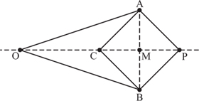
Figure 2.17. The Peaucellier cell.

Subtracting these gives

(OM)² − (PM)² = − ,

and rewriting the left-hand side as a product results in

(OM − PM)(OM + PM) = k²,

where k is a constant, and we have used k² = − for dimensional consistency. However, (OM − PM)(OM + PM) = (OC)(OP) and so we have

Hence we have shown that the product of the distances OC and OP is constant. So, if we choose OC, then OP = k²/OC. For this reason, if we have a curve along which OC moves, the curve which P follows is sometimes called an inverse of the original. We shall see in a moment that the inverse of a circle can be a straight line, thus solving our problem.

Now, to complete the linkage shown in figure 2.16 we add the final link QC with the condition that OQ = QC. We also ensure that O and Q are fixed points, so that the point C moves on a circle, centred at Q. Then, by theorem 1.1 we have that the triangle OCR is a right-angled triangle. Drop a perpendicular from P to the line OQ, and mark the meeting point N, then the triangles OCR and ONP are similar, so that

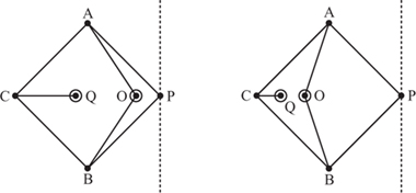
Figure 2.18. Alternative forms of Peaucellier’s linkage.

and so

Since the distance ON is constant, the motion of P must be a straight line, perpendicular to the line OQ.

In a more general case we must retain OQ = QC, but QC does not necessarily have to equal any of the short links l₂. It is a great convenience though in manufacture if the number of different lengths can be kept to a minimum. Peaucellier’s linkage is usually shown in the form of figure 2.16, but it can be made more compact by folding it in on itself. Using the same lettering we have the configurations shown in figure 2.18.

The geometry is unchanged, and according to Sylvester (1875a) it was in this folded form that the linkage was used to guide the piston rods on the ventilating engine in the old Houses of Parliament and by a wealthy resident of Southampton for the same purpose on the engine of a steam yacht.

The two key facts about Peaucellier’s cell are (i) that O, C and P remain in a straight line and (ii) that the product of the distances OC and OP is constant. This is sometimes called an inversor linkage. Any arrangement with these two characteristics will be sufficient to generate straight-line motion, for we can easily constrain C to move on a circle as before.

While Peaucellier’s linkage uses seven links, this number was reduced to just five by H. Hart in 1875, a model of which is shown in plate 5. Hart’s linkage uses a cell with just four bars and is shown in figure 2.19. This consists of a crossed parallelogram GHIJ, with GJ = HI and GH = IJ. This condition ensures that the (imaginary) lines GI and HJ remain parallel during the movement. Accordingly we shall take any other line parallel to HJ, and on each link we mark a point. We shall show in a moment that the marks on Hart’s linkage behave in such a way that the two important properties of Peaucellier’s cell are preserved. The diagram shows the case GH/GJ = . By similar triangles we have that

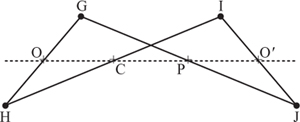
Figure 2.19. Hart’s inversor cell.

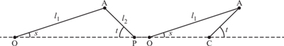
Figure 2.20. Hart’s ‘kite’ and ‘dart’.

If the linkage is moved then this property is preserved. Hence OP and CO′ will remain parallel with HJ. Since the distance of OP from HJ is GO/GH, and since this is also the distance of CO′ from HJ, the four points OCPO′ remain collinear during the motion of the linkage. This is the first important property of Peaucellier’s cell.

We are left to justify that OC · OP remains constant. One way to do this is to pull apart Peaucellier’s cell still further into two components (see figure 2.20). On the left of this figure we have half of a ‘kite’, and on the right half of a ‘dart’. It is then possible to match the dart with OHC and the kite with OGP, and we are done.

A direct argument can also be constructed from a result in geometry by noticing that the four points G, H, I and J of Hart’s cell all lie on a circle. In general three points determine a unique circle through them (or perhaps a straight line), so the fourth point being on this circle cannot be taken for granted. Hence, take the unique circle through HGI, then the perpendicular bisector of the chord GI passes through the centre of the circle, and by symmetry the point J also lies on the circle. A result known as Ptolemy’s theorem tells us, in the notation adopted for Hart’s cell, that

GJ · HI = GI · HJ + GH · IJ.

Since our links occur in two pairs we have that

GJ² = GI · HJ + GH²,

or

GI · HJ = GJ² − GH² = k²

for some constant k. By similar triangles, OC is proportional to GI and OP is proportional to HJ, so OC ·OP is also proportional to GI · HJ, and hence constant. These and other linkages have been given a case-by-case treatment. A general unified approach, in which these two occur as special cases, is given by Kempe (1875).

2.3 Hart’s Exact-Straight-Line Mechanism

We include one more mechanism invented by Hart which guarantees exact straight-line motion, and which moves in a most delightful way. It also uses only five bars, in two different lengths. Take five linkages with AC = BD = a, PC = PD = RS = b and attach the link RS to R and S so that the distance RC = DS = c, where b² = ac. The sketch in figure 2.21 shows the case where a = 8, b = 4 and so c = 2, which is a particularly convenient selection from a practical point of view. A model of this linkage is shown in plate 6.

Let us ignore the link RS for a moment. If we can arrange the other four links so that angle PCA equals PDB, then the two triangles APC and BPD will be congruent. Hence, AP equals PB and so point P will be found to move along the perpendicular bisector of AB. If we take RS = b and RC = DS = c, then we leave it to you to prove that the angle PCA equals PDB.

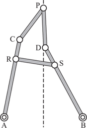
Figure 2.21. Hart’s straight-line mechanism.

Note that Peaucellier’s linkage can certainly be used to draw the ‘first’ straight line, since each link has only two pivots. However, to make either of the linkages shown in plates 5 and 6 it is necessary to create links with three collinear pivots. This presupposes the ability to place three points in a straight line.

2.4 Guide Linkages

This form of linkage relies on one of the pivots being itself guided in a straight line and the function of the other members is to magnify this movement so that one point on one of the links describes a much longer straight line. The point of this system is that although it requires a straight guide, this guide is considerably shorter and therefore easier and cheaper to make than a full-length guide. The best-known example is due to John Scott Russell (1808–82). He was an engineer and naval architect who, among many other activities, was associated with Brunel’s large steam ship the Great Eastern, a story told in more detail in Emmerson (1977). Scott Russell’s linkage is very closely related to the alternative form of Chebyshev’s linkage from section 2.1 and is shown in figure 2.22.

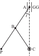
Figure 2.22. Scott Russell’s linkage.

Point A slides in a short straight guide GG, fixed point C lies on its centre line, and AB = BP = BC. Initially P is also on the line AC, and then moves so that AP is at some angle t to AC. Then P will have moved AP sin(t), while A will have moved only AP(1 − cos(t)). Of course, for this displacement of A, P can have swung from one side of AC to the other, giving a total of 2AP sin(t). The enhancement achieved is then

using a slightly old-fashioned trigonometrical term ‘versed sine’, equal to one minus the cosine. Putting some numbers in shows that for t =± 19° one foot of straight motion of P can be had from only about one inch of guide, a ratio of 12:1.

Scott Russell’s linkage occurs in all sorts of unexpected places once you start looking for it. Indeed, you may be carrying around an example in your car in the form of a car jack. In one popular design, the points C and P are connected by a long, threaded screw. The load of the car comes down on A. By rotating the screw, P is pulled closer to C, lifting the car. Here the mechanical advantage works in the opposite direction: a large horizontal movement of P causes a small vertical movement of A, making it easier to lift the car. A model of this linkage is shown in plate 7.

A slightly cautionary note here: suppose AP is a ladder resting against the side of a house, then the best way to stop it sliding down is to fix P. No matter how strong any rope securing B to C may be it is entirely useless.

Going back to the Scott Russell linkage we can see that the short guide GG could, in principle at least, be replaced by any of the linkages already described in this chapter. A Watt linkage for example gives a very close approximation to a straight line near to its centre of movement and would be quite suitable. Chebyshev experimented with arrangements, including those with his linkages. An engine using this arrangement was displayed at the Vienna Exhibition in 1873. Comments on this engine were reported in Engineering on 3 October (p. 284).

The motion is of little or no practical use, for we can scarcely imagine circumstances under which it would be more advantageous to use such a complicated system of levers, with so many joints to be lubricated and so many pins to wear, than a solid guide of some kind; but at the same time the arrangement is very ingenious and in this respect reflects great credit on its designer.

So, by the time of Scott Russell, in practice any gains that could come from replacing the guide by another Scott Russell linkage or other arrangement were not really worthwhile. There is one exception, though, that found application in medium-sized steam engines. It is based on the fact that a short arc of a large-radius circle does itself not deviate greatly from a straight line (shown in figure 2.23). In the form used in engines, D is fixed and a new link AD added. Point P guides the piston rod as it is driven by a vertical cylinder. It is known as the Grasshopper link because of the way link AD appears to vibrate when the engine is running. The place for this linkage should really be section 2.1 as P cannot move in a true straight line, but it is more appropriate to include it here with Scott Russell. A model of this linkage is shown in figure 2.13.

2.5 Other Ways to Draw a Straight Line

There are a variety of other ways in which a truly straight line can be drawn which do not involve link works. Just two are given here, the first of which involves one circle rolling around inside another. The second relies on two identical parabolas rolling around each other.

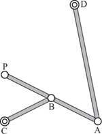
Figure 2.23. A Grasshopper linkage.

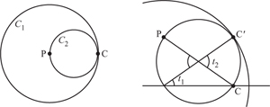
Figure 2.24. Rolling C₂ inside C₁.

Begin with two circles:C₁ of radius r₁ and C₂ which has half the radius, so 2r₂ = r₁. We roll the smaller circle around inside the larger one. Points on the perimeter of the smaller circle will be found to move in perfect straight lines. We begin in a configuration in which both horizontal diameters coincide. On the small circle mark two points: C where C₁ and C₂ touch, and P the point on the perimeter of C₂ which is also the centre of C₁. Note that C and P lie on the horizontal diameter of C₂. This is shown in the left-hand diagram of figure 2.24. Next we assume that C₂ has rolled around the inside of C₁, and this is shown, enlarged, in the right-hand diagram, so that the line which joins the centres of C₁ and C₂ makes an angle of t₁ with the horizontal.

We now have a new contact point, C′, between C₁ and C₂, and we consider the angle t₂ between the two radii in C₂ connecting the horizontal to C′. As we have assumed that there is no slipping between the two circles C₁ and C₂ as they roll, the arc length from C to C′ on C₁ must equal that from C to C′ on C₂. Arc length is the product of radius and angle, l = tr (measured in radians of course). Since r₁ = 2r₂ we have that

r₁t₁= l = r₂t₂,

or, since 2r₂ = r₁,

2r₂t₁ = r₂t₂,

so that t₂ = 2t₁.

From this it is clear in the diagram, and can easily be confirmed by elementary geometry, that the point C remains on the horizontal diameter of C₁. Since t₁ is arbitrary in this argument it follows that the path of C is a horizontal straight line. Indeed, an identical argument shows that the point P moves along a vertical straight line, and indeed each individual point on C₂ moves in a straight line. This observation has been used with a small cog wheel inside a larger one to generate straight-line motion. Such a contrivance is that patented by James White in 1801 (see figure 2.25). One problem with this mechanism is the great strain on the central bearing, and it was not particularly widely used.

The next method for drawing a straight line is, admittedly, somewhat contrived. Nevertheless it does illustrate one property of the parabola that we learned how to cut out in section 1.4. There we gave an algebraic equation of the parabola in the form y = x²/(4a). First we consider the parabola from a geometric, rather than an algebraic, point of view. Let us take a point P on the parabola, which of course has coordinates

Again, we use the Pythagorean theorem to find the distance of this point from the coordinate (0, a). This turns out to be

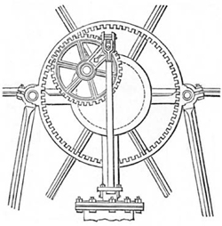
Figure 2.25. James White’s parallel mechanism.

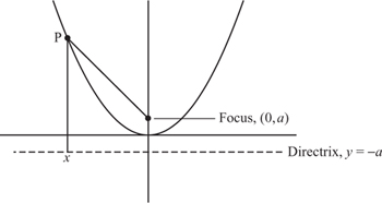
Figure 2.26. The focus–directrix approach to the parabola.

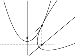
Figure 2.27. Two identical parabolas.

which is precisely the distance from P to the horizontal line y = −a. Hence, we can show that the parabola is the locus of points that are the same distance from a given fixed point (0, a) as they are, perpendicularly, from a line y = −a. The fixed point is called the focus of the parabola, and the line the directrix (see figure 2.26). Indeed, the parabola is more traditionally defined as the locus of a point which moves so that its distance from a fixed point is equal to its perpendicular distance from a fixed straight line. From this its equation is derived. This explains the slightly strange looking factor of 1/(4a) that we gave in the defining equation of the parabola.

What we now do is take two identical parabolas, one of which we assume is fixed. The second is made to roll around the first, with the condition that it does not slip. This configuration is shown in figure 2.27. There is a natural symmetry between the two parabolas, with the focus of one always lying on the directrix of the other. This means that if we place a pen on the focus of the moving parabola, it will draw a straight line as one parabola rolls around the other.

We have experience of trying to draw a line in this manner using the two parabolic plywood templates shown in plate 9. It is extremely difficult to do and is at least a three-hand job.