Chapter 11

PLENTY OF SLIDE RULE

Yet I confess I like it the better, because it pleaseth not your palate, to which nothing can savour, that is learned and Analyticall: but onely the superficiall scumme and froth of Intrumentall trickes and practices.

Oughtred (1634)

 

 

We want to ask you to imagine you are the captain of a supertanker that is docked in port and being loading with oil. Your tanker has a number of separate tanks, perhaps of different volumes, and oil is being pumped aboard. If you decide to fill one tank at a time then the ship will capsize, so you need to balance the ship by part-filling tanks around the vessel. Oil varies in density, and so you cannot rely on a set of pre-prepared tables since you may not know how heavy the oil is until you start the job. What you need to help you do this is a simple, reliable and quick method of performing these volume, density, flow rate calculations on the deck of your ship.

There has always been a need to perform such calculations: they were used by ships’ captains, carpenters and tax collectors, among others. Remember that space flight predates by some decades the cheap mass-produced electronic calculator. Most modern computers are digital; however, there are a number of devices for calculating that rely on continuously changing physical quantities. Such devices are known as analogue computers. These quantities might be water flow rates, electrical voltages or the physical position of a mechanism.

Such devices were widely used for practical calculations which did not need more than two or three significant figures of accuracy, and it is precisely one of these that William Oughtred dismisses above as ‘the superficiall scumme and froth of Intrumentall trickes’. Indeed, the quotation is one salvo in a bitter argument over the priority for the invention of analogue devices that use length and angle as the physical quantities. These are known as slide rules, and they rely on the relative physical positions of two scales. Such devices are the subject of this chapter.

Figure 11.1. Setting two logarithmic rulers to perform 2 × 3.

Have a look at the rules shown in figure 11.1, which are set up to perform the multiplication 2 × 3. The first thing to notice is that the scales themselves are not equally spaced. Actually they are drawn using logarithms and reading a logarithmic scale does take a bit of practice. Notice that the distances between the marks are uneven and that there are more marks between 1 and 2 than between 9 and 10. If you count, you will find that between 1 and 2 there are forty-nine marks but between 9 and 10 there are only nine.

We shall explain how to use the slide rule using examples, starting with the simple product 2 × 3, which may be calculated by using the two logarithmic rulers shown in figure 11.1. The two scales have been labelled C and D as these letters are traditionally used on slide rules for the scales shown here. Place them side by side so that the 1 on C is next to the 2 on D. Now look on C for the 3. The answer to the product 2 × 3 is the value that is opposite this 3 on the D scale, as shown in figure 11.1. What we have actually done is added the logarithm of 2 (on the D scale) to the logarithm of 3 (on the C scale), and this process will be fully explained in section 11.1. Notice that without moving the ruler we may calculate lots of other products. For example, we can read 2 × 4 and 2 × 5 off the slide rule without touching either ruler. This feature actually makes the slide rule quicker to use than the electronic calculator for some repetitive tasks, such as converting a student’s homework mark to a percentage, at a glance.

11.1 The Logarithmic Slide Rule

Just as in the above example, the most common use of a slide rule is to perform multiplication (or division) based on the laws of logarithms. If x > 0 then the logarithm of x to the base a > 0 is the unique number y that satisfies

a^y = x.

This is written as y := log_a(x). For example, 10³ = 1000, so log₁₀(1000) = 3, and 2⁶ = 64, so log₂(64) = 6.

From this it follows that

In practice a is taken to be 10 or the special number e ≈ 2.71828. This latter base gives what are called the natural logarithms, which become important mathematically from calculus onwards. They are often denoted by ln(x) rather than log_e(x).

Taking a = 10 is usual in practical calculation because of the following link with number bases in the place–value number system. If we work through the above definition of logarithm it is straightforward to see that

log₁₀(10y) = 1 + log₁₀(y).

Now, repeated use of this together with (11.1) gives

log₁₀(100) = 2, log₁₀(1000) = 3, ..., log₁₀(10^y) = y,

and so log₁₀() = −1. Often we simply write log in place of log₁₀ where there is no risk of ambiguity.

The crucially important property of logarithms derives directly from the law for exponents that

a^y a^z = a^y+z,

and they allow us to convert a multiplication into addition using the relationship

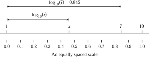
Figure 11.2. Drawing a logarithmic scale.

The invention of the logarithm by John Napier in 1614 was perhaps the most important advance in practical calculation since the introduction of the place–value (decimal) number system. Napier was a colourful and inventive character. Amongst his other writings, Napier published A Plaine Discovery of the Whole Revelation of Saint John in English in 1593. This contained proofs, in the style of Euclid, that the pope was the Antichrist and that the world was due to end in 1786. What we remember Napier best for is the small book, first published in 1614, entitled Mirifici Logarithmorum Canonis Descriptio (‘Description of the Wonderful Canon of Logarithms’). This book was a set of tables and a short description of how to use them. An explanation of the theory and the method of calculation was published posthumously in 1619 as Mirifici Logarithmorum Canonis Constructio (‘Construction of the Wonderful Canon of Logarithms’). This was translated subsequently by Henry Briggs and published in English. It should be noted that Napier’s concept of logarithm was quite different, although of course mathematically related, to (11.2). More details of this may be found in, for example, Edwards (1979).

Although logarithms now appear modestly as a button on an electronic calculator, their effect on the seventeenth-century scientific community was profound. In Napier’s time, the concept of a fractional exponent had not been developed and neither had the general concept of a function—it would therefore have been impossible for Napier to have given the synopsis of logarithms that we have done. Hence Napier’s definition differed from ours and was based on the continuous movement of two points. Without calculus this was the only way of considering continuously varying quantities. When Johannes Kepler (1571–1630) received a copy of Napier’s tables, he used them to assist him with the calculations that led to the formulation of his laws of planetary motion. Without the aid of logarithms these calculations would have taken many years, and Kepler published a letter addressed to Napier as the dedication to his Ephemeris of 1620 congratulating him. In turn, Kepler’s laws gave Newton evidence that was crucial to support his theory of universal gravitation. With this in mind we get some idea of the significance of Napier’s discoveries.

To implement the mathematical law (11.2) physically, we need to draw logarithmic scales. On such a logarithmic scale the physical length from the origin is proportional to the logarithm of the number marked on the scale. For example, log(1) = 0 and so the 1 is marked at the origin of the scale. To make a logarithmic scale, first draw a line and mark two points on it. These will correspond to the numbers 1 and 10. To mark a point on the scale, 7 for example, we measure a length proportional to the logarithm of 7 along the line. This is illustrated in figure 11.2. A completed logarithmic scale is show in figure 11.3.

In chapter 4 we made much of the difficulty in accurately constructing a scale by pure geometry, without any measuring whatsoever. Unfortunately, apart from the ends 0 and 1, none of the positions of the other points can be established by construction. The procedure undertaken by practitioners such as Stone (1753) began with dividing a scale up into equal parts, perhaps 1000. Once this was complete a table of logarithms was used to find the position of each mark. The positions of prime numbers could be used to establish the other marks. For example, if we mark out the positions of 2 and 3, addition of the physical lengths by geometrical construction allows us to find the positions of 4, 6, 8, 9 and so on. However, this procedure risks the introduction of cumulative errors when the slide rule is being marked out by hand by a craftsman. Rules would originally have been marked out in this way but craft production eventually gave way to mass production.

Figure 11.3. A logarithmic scale.

Figure 11.4. The principle of a slide rule.

In the opening section of this chapter we calculated the product 2 × 3 by using two logarithmic rules. In effect we had added the lengths, and hence added the logarithms of the numbers. Since (11.2) assures us that adding logarithms corresponds to multiplying the numbers, we can now see the principle of the logarithmic slide rule. This calculation is shown again in figure 11.4 to emphasize the addition of physical lengths.

Although it is possible to perform many other similar calculations immediately, it is impossible to calculate 2 × 6 because we run out of scale. If you ever run out of scale like this you need to divide by ten. This corresponds to moving the whole of the C ruler to the left so that the 10 on the C is where the 1 currently is, as shown in figure 11.5. The 6 on C is now above 1.2 on D but we divided by ten so the answer must be 12, which is, of course, 2 × 6. Similarly we can read off 2 × 7, 2 × 8, etc., the scale reading being multiplied by ten.

It is possible to design a circular slide rule in which the angle, not the length, is proportional to the logarithm—we shall examine circular rules in section 11.4. The problem of insufficient scale does not occur with a circular pattern rule, although the position of the decimal point must still be established by mental calculation. In fact, when using a slide rule the decimal point must always be established by mental arithmetic. Hence, the rules in figure 11.1 may just as readily be used to calculate 2 × 3, as 200 × 0.03.

Figure 11.5. Setting two logarithmic rulers to perform 2 × 6.

Division may be performed equally simply, essentially using the reverse process by noting that (11.2) may be rewritten in the form

log(y) − log(z) = log for all y, z > 0.

If we begin this time with y on the D scale and locate z on the C scale, the difference between these two logarithms will be the logarithm of y/z. Figure 11.4 can be reinterpreted to show the rule set-up for 6 divided by 3. Look at figure 11.5: in this, the 7 on the C scale is above the 1.4 on the D, so this configuration is precisely that needed to calculate 14 ÷ 7, and the 10 on C is indeed above the correct answer, i.e. 2, on the D scale.

The basic principle of the slide rule is simple—however, there are a number of subtleties in its practical operation that require skill together with manual and mental dexterity. Next we examine the history of the slide rule and then, in section 11.3, we explain how other common calculations are performed, often with the aid of different scales. This only scratches the surface of an extensive field, albeit a rapidly dying one.

11.2 The Invention of Slide Rules

The slide rule is an extremely good case study of how the development of technology progresses in small incremental steps rather than by large leaps. Originally, a single logarithmic scale was inscribed upon a rule by a craftsman using a table of logarithms to establish the positions of the individual marks. A pair of dividers was used to walk along this single scale to add lengths. Next, two rulers were placed side by side on a desk, just as in figure 11.1. From this a gradual refinement of the tool took place with the introduction of a sliding cursor, better scale layout and new materials. Every step represents a genuine improvement, although each one by itself seems rather unimportant. The sum total is a sophisticated, accurate and highly versatile instrument. One could expect a late-twentieth-century general-purpose slide rule to be inscribed with up to thirty different scales aligned on both sides.

The first scientific instrument to contain a logarithmic scale was the sector, which was discussed separately in section 4.6. This innovation is credited to Edmund Gunter, who became Gresham Professor of Astronomy in 1619. His most important book was his Description and Use of the Sector, which was first published in English in 1623. This was hailed by Cotter (1981) as ‘the most important work on the science of navigation to be published in the seventeenth century’. Now, Gunter’s sector is not a slide rule in any sense of the term. It contains a single logarithmic scale that is used in conjunction with a pair of dividers. Imagine that we wish to perform a multiplication calculation, for example. Begin by opening the dividers a distance corresponding to the logarithm of one number, as measured on the scale. Then place one point on the scale itself at the point corresponding to the other number and see where on the scale the other point comes into contact. We have added lengths by using the legs of the dividers.

The actual invention of the slide rule came next, and like many of the devices described in this book, its priority for invention is a complex issue, involving a controversy between two rival inventors: William Oughtred (1573–1660), whose detailed biography is Cajori (1916), and Richard Delamain (1610–45) (see Taylor 1954, section 122). It is generally accepted that Oughtred was the inventor of the first slide rule but that Delamain published first, and, furthermore, that the two probably independently invented their instruments (see Cajori 1920, p. 205). The first published account of a circular slide rule is to be found in Richard Delamain’s 30-page pamphlet Grammelogia of 1631. This was closely followed by William Oughtred’s The Circles of Proportion and the Horizontall Instrument (Oxford University Press, 1632). Note that the ‘horizontall instrument’ is a form of sundial not slide rule (Turner 1981). Translated and published for Oughtred by William Forster (Taylor 1954, section 164), the introduction attacks Delamain. Delamain’s expanded 113-page Grammelogia of 1632 replies to the attack contained in the introduction to Circles equally forcibly. In 1633 Oughtred published an edition of Circles with a section titled ‘Hereunto is annexed the excellent Use of two Rulers for Calculation’. This details the linear slide rule for which Oughtred has undisputed priority. The 1634 edition of Circles contains the 32-page section with the following title.

TO THE ENGLISH GENTRIE and all others studious of the MATHEMATIKS, which shall be Readers hereof. The just Apologie of WIL: OUGHTRED, against the slanderous insimulations of RICHARD DELAMAIN, in a Pamphlet called Grammelogia, or Mathematicall Ring, or Mirifica logarithmorum projectio circularis.

This section is referred to as Oughtred’s Apologie and we shall examine the argument between Oughtred and Delamain in more detail in section 11.9, since their views on using calculating instruments in teaching are fascinating, and still relevant.

The further development of the slide rule cannot really be isolated from that of other scientific instruments. Indeed, all instruments of this period were hand inscribed, making them very expensive and possibly inaccurate. Also, instrument makers in the early seventeenth century understandably guarded their trade secrets very carefully. Such secrecy not only reduced communication of ideas but inevitably led to independent reinventions. This sparked controversy, although both Oughtred and Delamain used the same instrument maker, Elias Allen. It was not until 1753 when Edmund Stone published his Construction and Principle uses of Mathematical Instruments that such information began to become available. The work of Hopp (1998) divides the history of slide rule manufacture into approximately two periods. The first was from the 1630s to the 1850s. This is characterized by individual instrument makers, each with their own patterns for the scale layouts and innovations in the physical design. From the 1850s onwards the patterns of scales became more standardized and manufacture and mass production became more common. The introduction of better materials, specifically printed celluloid scales and plastics, brought the costs down and improved accuracy, making the slide rule a useful and affordable tool. We shall sketch out some of these important innovations below.

Although an apparently obvious idea, it seems that it was not until 1654 that Robert Bissaker thought of placing a slide between two fixed stocks rather than simply placing two rules side by side on a desk. This is the first recognizable slide rule, although the name does not appear until 1662 when John Brown used the term in a book. During the later seventeenth century standard designs began to emerge, such as those of Coggeshall and Everard.

Physical innovations continued, as did different arrangements of scales until the pattern most commonly found on modern slide rules was first invented by Amédée Mannheim (1831–1906) around 1850. His rule also contained a cursor, which allows one to read scales that are not contiguous accurately. Although this was invented in England two centuries earlier by Newton, on the device examined by Sangwin (2002), it only became popular with Mannheim’s rule.

Mannheim’s rule is based around two logarithmic scales, one on the slider and one on the bottom of the stock, which are traditionally labelled C and D, respectively. In addition, two other scales marked A and B contain double logarithmic scales. That is to say, if a reading x is taken on the D scale, directly above this is the reading x² on the A scale. The other most common scales are K, a triple scale at the top of the rule, and the scale CI on the slider, which is an inverse scale. Trigonometrical relationships are generally given on the reverse side of the slider.

Following Mannheim’s rule innovations continued, including the addition of a magnifying glass to the cursor. Different physical designs became popular, including pocket watch circular calculators and cylindrical calculators. Other scales such as the log–log scale were introduced. The duplex rule—that is, a rule with scales aligned on both sides—was patented in 1891 by William Cox (US Patent 460930). The folded scales, which will be explained below, were introduced by Auguste Beghin in 1898. Development and mass manufacture of slide rules continued until the late 1980s, with the last rules produced designed for special applications. Some rules, such as the Moonstick, which as the name implies is used for calculations involving phases of the Moon, are still available.

Figure 11.6. A typical slide rule, the Faber Castell 67/87 Rietz.

11.3 Other Calculations and Scales

In addition to two simple logarithmic scales, an early twentieth-century slide rule traditionally came equipped with a number of others. These are designed to facilitate a variety of calculations, including trigonometrical ones. In this section we look at just a couple of the more common scales to give you some idea of the range possible. Most slide rules came with instruction manuals, which have the advantage of relating example calculations to the actual scales on the rule. In addition, there are many general instruction manuals: see, for example, Dobson (1972) and Snodgrass (1959).

In the multiplication calculations illustrated in figure 11.1 we soon ran out of scale, i.e. 2 × 6 cannot be found. One solution to this problem was first used by Auguste Beghin in 1898 and is known in its modern form as the folded scales. To use the folded scales we need to move away from two juxtaposed scales and imagine a number of different scales on both the fixed stock and the moving slider. In fact we imagine that the C and D scales are continued to the right. This would evidently solve the problem. The extensions to the C and D scales are cut off, and labelled CF and DF, respectively. These two new scales are displaced physically back to the left, so that the C and CF scales are on the slider and move together. The D scale is contiguous to C, usually on the bottom of the stock, whereas the DF scale is contiguous to CF on the top of the stock.

Figure 11.7. Using the scales CF and DF to perform 2 × 6.

However, the CF and DF scales do not begin at 1. In fact, they begin about halfway along the physical scale. Mathematically, half the physical distance along the scale corresponds to 10¹/2 = ≈ 3.1623. Actually, a more popular displacement for the folded scales is π ≈ 3.1416, which by chance is approximately , but more useful in calculations.

Since the C and CF scales are fixed together on the slider and the D and DF scales are fixed together on the stock, any calculation performed on the C/D scales will also be performed on the CF/DF scales. However, the portion of the scales that is visible will be different. So, if we return to our calculation of 2 × 6, we cannot read the answer by looking below the 6 on the C scale because we have run out of D scale. Instead, we can look above the 6 on the CF scale and find the 12 on the DF scale. This is illustrated in figure 11.7. In ways similar to this, we can use combinations of the C/D scales and the CF/DF scales to ensure that the result appears on one of the scales. This is difficult to describe in words, but is actually evident with a little practice.

Two other scales that commonly appear on slide rules are labelled A and B, with A fixed on the stock and B on the slider. Both of these fit two complete scales into the physical distances occupied by the C and D scales. Therefore, by the laws of logarithms, the A scale shows the square of the D scale, and similarly the B scale the square of the C. Since squaring and taking the square root of a number are very common functions, the usefulness of this is evident. However, since the A and B scales occupy only half the physical space, they have only half the accuracy. In using these scales for squares and square roots, real care is needed in determining the position of the decimal point.

The real power of this arrangement is when calculations on the C/D scales are combined with calculations on the A/B scales. To ensure the maximum overall accuracy, it is important to minimize the total number of slider movements and intermediate calculations. To achieve this a calculation must be planned in advance. The cursor can be used to ‘store’ an intermediate result, while the slider is moved. This removes the need to note down such a result on paper. On a late-twentieth-century rule both sides are used and the scales on each side are aligned. On both sides the C/D scales appear, with A/B scales on one side and CF/DF scales on the other. By turning the rule over and using both sides simultaneously in a calculation, the best use can be made of all the scales. In doing this the cursor is invaluable for transferring a number from one side to the other.

Some numbers, such as π, occur regularly in calculations. As in figure 11.7, such values are marked on a rule for speed and accuracy and are known as gauge points. Gauge points are specific values that are marked on the rule to help with specific calculations. Two other common gauge points are marked ′ and ″: these show, respectively, the factors for multiplying minutes and seconds of arc to turn them into radians. Which other gauge points are present depends very much on the intended user of the rule. For example, carpenters, tax officials and accountants all had their own gauge points for helping with calculations relevant to their professions.

Another common feature on slide rules is an extra hairline on the cursor of the rule. This is offset by a fixed distance and allows for a multiplication factor to be immediately calculated. The most common auxiliary hairline appears to the left of the cursor hairline for use with the A/B scales. This corresponds to a multiplication factor of π/4 ≈ 0.785. Since the area of a circle is (π/4)d², this auxiliary hairline is invaluable for this common calculation. To perform this, move the cursor to the diameter on the D scale, and read the square of this on the A scale above. Then, looking at the position of the auxiliary hairline, find the area on the A scale. Note that for this calculation the slider is not needed. Similarly, a tax inspector might have an auxiliary hairline at 1.175 to allow addition of a tax of 17.5% very accurately and swiftly.

There are also scales for trigonometrical calculations. For example, if one needs to calculate a × sin(t), then one adds the length corresponding to log(a) to that corresponding to log(sin(t)), which may be read directly from one of the other scales. Unlike an electronic calculator that copes with the periodicity of the circular functions, the user needs to do much more when using a slide rule. The sine of an angle is usually only given for 0 ≤ t ≤ 60^°, and a user would be expected to convert values of t into this range before picking up the rule. This can be done by using trigonometrical relationships such as sin (90^° − t) = cos(t).

11.4 Circular and Cylindrical Slide Rules

The linear slide rule is only one possible layout for the scales. Indeed, Oughtred’s original design was circular. Although significantly less common than the linear slide rule, both circular and helical cylindrical slide rules were produced. The helical slide rule in particular has a much greater scale length and hence is far more accurate than its linear counterpart. A circular slide rule with conversion tables, the ‘Concise Type E’, is shown in figure 11.9.

The most significant advantage of the circular design is that one does not run out of scale. The calculation continues around the circle, with the user keeping track of the decimal point as with the linear rule. Circular designs have another advantage: by wrapping a scale round a circle we get just over three times as much scale on a circle of given diameter as we do on a straight rule of that length, and the helical slide rules had an even greater scale length. For example, the Otis–King calculator, which was patented in 1922, has a scale length of 66 in wrapped around a cylinder approximately 2 in long and 1 in in diameter. Details of the scale are shown in figure 11.10.

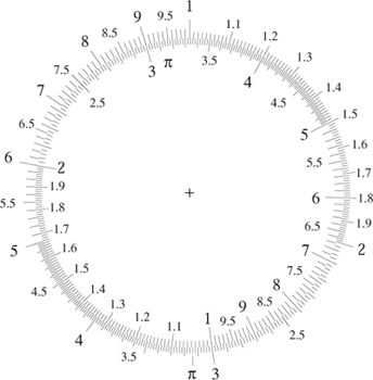
Figure 11.8. Circular rule set to multiply by three.

As an example of a circular layout, we can place one scale inside another. The two scales in figure 11.8 are set up in such a way that we can use them to multiply by three. The 1 on the inside is next to the 3 on the outside. Similarly, the 2 on the inside is next to the 6 on the outside. We can see that the advantage of a circular configuration is that we do not run out of scale when we come to 4 on the inside, which is next to the 1.2 on the outside. Since we have gone round the outside once this corresponds to 12, which is the correct answer. So, just as with a linear rule we still need to keep track of the decimal point.

11.5 Slide Rules for Special Purposes

As mentioned, most slide rules have gauge points that indicate constants to aid specific calculations, π being an example. A special slide rule is one that has whole scales inscribed in such a way that calculations relating to specific problems can be resolved quickly, simply and accurately. They have the advantage that a problem can be resolved almost as quickly and with little more trouble than it takes to write the numbers down. In some circumstances this can be very important: when a flight heading has to be corrected to account for prevailing winds, for example. Furthermore, a specific scale can be more accurate than using a general scale. For example, for a calculation involving barometric pressure at or around sea level, numbers in the range 710–770 (millimetres of mercury) will be used. This range is compressed into less than 15 mm on a general-purpose 300 mm rule. A slide rule is also less bulky than a chart or graph.

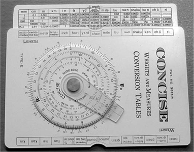
Figure 11.9. A circular slide rule with conversion tables, the ‘Concise Type E’.

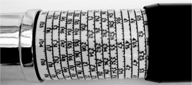
Figure 11.10. Detail of the helical scale on the Otis–King calculator.

Figure 11.11. A general slide rule schematic.

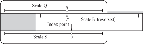
Figure 11.12. The usual scale layout on a special slide rule.

Of course, a special rule can be used for only one problem, or at most a very limited number. They are complicated and difficult to produce, especially when the scale markings are calculated by hand. This is a serious flaw and limited the range of applications in which special rules were used. Finally, suitable blank rules were difficult to obtain by non-specialist manufacturers. Despite these problems, many special rules were constructed and used. The following section briefly describes the theory and examines a particular case study: an oil tonnage calculator.

Special rules operate by adding lengths proportional to the values of the functions represented on their scales. For example, the scheme shown in figure 11.11 solves

where length Q = f₁(q), length R = f₂(r) and length S = f₃(s). The scales are marked with numbers q, r and s. If f₁, f₂ and f₃ are all logarithms, then (11.2) becomes precisely (11.3), and we have the usual configuration for multiplication.

In order to prevent confusion over which scales to use, we assume that scale S contains the unknown, which is to say the desired answer. It is then easiest to draw Q on the upper part of the stock and R contiguous with Q on the slider. The result is then read from scale S using a cursor or an index line on the slider. When constructing a special rule, we may not have a cursor available. If this is the case we have to use a fixed index point, rather than a moving cursor. To do this it is necessary to arrange the scales slightly differently. In particular, the scale R needs to be reversed. The r in figure 11.11 will then appear directly below the q, and the index point will be below scale R and directly above scale S: see figure 11.12. Apart from removing the need for a cursor, there are other advantages to this arrangement. Reversing the direction of scale R, and the flexibility we have in placing the index point, means that we are less likely to run out of scale S using this configuration. Taking a proportional scale for each of scales Q, R and S reduces (11.3) to

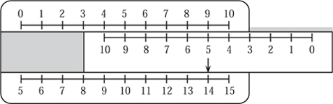
Figure 11.13. A slide rule for sums.

Q + R + S.

Now, taking S to be the unknown, we can devise a rule for adding numbers. This is shown in figure 11.13 and illustrates the reversed scale R. In this example, one immediately notices many different sums that total 14.

For an example of a reversed scale on a normal slide rule, look for the scale CI, which is usually drawn on the slider, often in red. This corresponds mathematically to 1/x, and since log(1/x) = −log(x), graphically this corresponds precisely to a reversed copy of the principal scale C. To multiply with this using the layout of scales illustrated in figure 11.12, imagine a copy of the usual D scale occupying the position of scale Q. Use the CI scale as scale R and take the 1 on the C scale as the index point.

The answer to normal multiplication of q and r can be read off directly using the index point and the D scale. What we have actually done here is divided by 1/x, as represented on CI, which is of course multiplication.

For another example, using the standard slide rule, take scale Q as the scale A (the squared scale, x²), R is the CI scale (1/x), and take π as the index point on the C scale. Setting the slider for numbers on scales Q and R, the answer on the bottom scale is s = πr .

This is not the place to explain the intricate arrangements of scales in more complex rules or the techniques for efficiently laying these scales out. Such details can be found in the work of Hoelscher, Arnold and Pierce (1952).

11.6 The Magnameta Oil Tonnage Calculator

As an example of a special rule, consider the Magnameta oil tonnage calculator, which is a slide rule specifically constructed to deal with the problems relating to the loading of oil tankers. Imagine trying to balance the ship as oil of a specific density flows into tanks of various sizes positioned in various places around the ship. The trick is not to capsize the boat during this process. As the instruction book says,

[i]t is intended primarily for use in handling loading problems, when the ability to estimate the weight per tank with speed and accuracy is of prime importance.

It continues as follows.

The rule, which in spite of its size is neither heavy nor cumbersome, carried under the arm, is the answer to this problem. The official figure must under these circumstances be worked out later.

The rule is of standard design, as shown in figure 11.12, with a single slider and a cursor. The instrument has five scales denoted A–E. The primary scales A and E are marked on the stock and measure 783 mm in length. The other scales are marked on the slider and measure 381 mm. Scale A is the tank capacity, calibrated from 15 000 to 50 000 cubic feet. Scales B and C are international specific gravity values from 0.6 to 1.08. These are reversed logarithmic scales running from 33.292 to 59.972 with markings giving the specific gravities. The reversal of these scales is exactly as in figure 11.12. The D scale is marked in American petroleum industry (API) specific gravity values, and E is calibrated in tons for values between 450 and 1500 tons per tank.

The cursor has three lines, marked I, II and III from right to left. Lines II and III correspond to multiplication by 1.015 and 1.12 and the three lines allow calculations in long or short tons or in metric tonnes, respectively. The cursor is also fitted with a clamping device that holds it in one place relative to the slider. Loading problems always involve oil of a fixed specific gravity so being able to accurately fix the cursor has obvious advantages. Essentially the moving cursor becomes a fixed index point.

To perform a calculation, the cursor is fixed at a specific gravity and then the slider, with fixed cursor, is moved to a corresponding volume on the top scale A. The weight is read directly off scale E using the appropriate index point. This is exactly as described in section 11.5 above. The rule can be used for tanks calibrated in water tons and cubic metres (metric water tonnes) by using lines II and III on the cursor. Weight to volume calculations are straightforward using the reverse process. Lastly, API specific gravities can be converted to International specific gravity units by allowing the cursor to run freely and reading across scales C and D.

United Kingdom Patent 919063 was granted to the inventor Guy William Farrier Sangwin, the complete specification having been published on 20 February 1963 (Sangwin 1963). The calculations for the scale and the printing of the plates took three years to complete. The prototype rule, with scales printed onto plastic and laminated onto a wooden base, survives although the leftmost 150 mm of scales A and E have been badly damaged by water (the rule was rescued from a garage). This is shown in plate 23. The introduction of cheap electronic calculators in the 1960s prevented this particular rule being produced commercially.

11.7 Non-Logarithmic Slide Rules

Slide rules and logarithms are inextricably linked, so it may come as a surprise to discover that to produce a slide rule capable of multiplying two numbers it is not necessary to use logarithms at all. We use this as another example of a special slide rule, since the construction exactly follows that in section 11.5. The original idea for this comes from Mills (1958).

Section 6.1 introduced the triangular numbers

1+ 2 + ··· + n = n(n + 1).

Instead of taking a whole number n, define for any positive number x the function

Δ(x) := x(x + 1).

Then, by elementary algebra, we have that

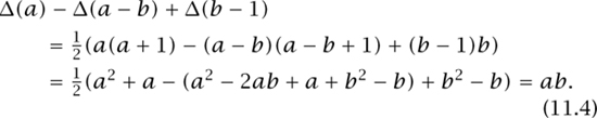
Given a and b, by calculating Δ(a) − Δ(a − b) + Δ(b − 1) we may calculate ab (notice the similarity with (11.3)). It is on this observation that the ‘Nelson rule’ relies. By drawing scales proportional to Δ(x) (instead of log (x) as in a logarithmic slide rule) we may design a slide rule. The scales are drawn as follows: the top scale is proportional to Δ(a), the top scale of the slider is proportional to Δ(a − b), the bottom scale of the slider is proportional to Δ(b − 1), and the bottom scale on the stock is a simple proportional (equal division) scale.

Such a rule, set up to multiply 8 by 3, is shown in figure 11.14. Set up the rule with the a − b = 8 − 3 = 5 on the top slider scale adjacent to the a = 8 on the top scale. Look at the b = 3 on the lower scale. This is above the answer, 24, on the proportional scale. That Nelson’s rule works for arbitrary positive numbers and not simply whole numbers is obvious if looked at from the point of view of the algebra in (11.4), rather then by viewing Δ(x) in terms of triangular numbers. Nelson’s rule may actually be simplified, since algebra also confirms that

Figure 11.14. Nelson’s rule.

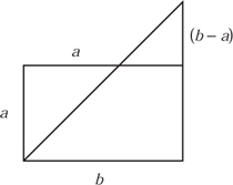
Figure 11.15. Geometrical interpretation of improvements on Nelson’s rule.

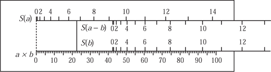
Figure 11.16. Improvements on Nelson’s rule: 11 × 5.

a² − (a − b)² + b² = ab.

Comparing the areas of the triangles and rectangles shown in figure 11.15 confirms this geometrically. By using an almost identical construction, this time using the function

S(x) = x²

in place of Δ(x), we arrive at the slide rule shown in figure 11.16. This rule is set up to calculate a × b = 11 × 5 by setting a = 11 on the top scale adjacent to the a − b = 6 mark on the slide. The answer is read below b = 5 on the lower scale. The symmetry between a and b in the product a × b is more evident in this construction than in Nelson’s. No doubt other relationships along similar lines are possible.

11.8 Nomograms

A related topic is that of nomographs, or alignment charts. These were frequently used for routine engineering calculations and the example we take is typical of the many that were in common use. It relates the volumetric flow rate of a gas to the nozzle diameter and the supply pressure. It consists of equispaced vertical logarithmic scales graduated in the accepted units: pressure in inches of water and flow rate in cubic feet per hour. The scale on the nozzle diameter axis looks more like an irregular arithmetic scale of numbers with no units on one side with a size in inches against each number on the other. Drills are available only in standard sizes and the number refers to those drills widely used for all sorts of purposes and still used by some model engineers. It would be pointless and prohibitively expensive to have to make a special drill to a calculated diameter for every nozzle.

As the name alignment chart suggests, it is used by placing a straight edge between the variables to find the value of the third. This is a quick and virtually foolproof way of doing a particular calculation.

An early example of a nomogram is a method devised by Sir Isaac Newton for approximating roots of polynomial equations using slide rules. It first appears in Newton’s ‘Waste book’ (see Whiteside 1961) around 1665. The method appears to have then been explained to John Collins in a letter of 1672. Collins was interested in finding the volume of liquid in a partially full barrel as a function of depth.

Wherefore since I understand your designe is to get a rule for guageing vessells, this Problem having so bad success for yt end I shall in its stead present you with this following expedient.

Turnbull (1959–61, volume 2, p. 229)

This was an important issue in gauging, i.e. the calculation of various taxes on liquids. Interestingly, slide rules were particularly popular amongst customs officials, for whom they provided an instant volume calculation, by visual inspection, and therefore instantly settled the question of how much tax or duty was due. It is reported in Whiteside (1961) that this method was incorporated by Collins into a general method for solving cubic equations. Collins then wrote In Answer to Mon^r Leibnitz’s Letter about Solving a Cubick Æquation by Plaine Geometry. This ‘answer’ was passed to Oldenburg, who, in the following letter dated 24 June 1675 (quoted in Cajori (1909, p. 21) but also in Horsley (1782, VI:520)), communicated the ideas to Leibnitz.

Mr. Newton, with the help of logarithms graduated upon scales by placing them parallel at equal distances or with the help of concentric circles graduated in the same way, finds the roots of equations. Three rules suffice for cubics, four for biquadratics. In the arrangement of these rulers, all the respective coefficients lie in the same straight line. From a point of which line, as far removed from the first rule as the graduated scales are from one another, in turn, a straight line is drawn over them, so as to agree with the conditions conforming with the nature of the equations; in one of these rules is given the pure power of the required root.

The theory is described briefly in Cajori (1909), and reference is made to Stone (1743) in which ‘Newton’s mode of solving equations mechanically is explained more fully and with some restrictions, rendering the process more practical’. Both the linear and circular versions are discussed in more detail in Sangwin (2002). We have used this technique, but it is not easy.

11.9 Oughtred and Delamain’s Views on Education

We digress slightly in this section and comment on Oughtred and Delamain’s views on education. We know something of these because of the priority dispute for the invention of the slide rule (discussed in section 11.2). Delamain, originally a joiner but later a ‘teacher of practical mathematics’, was eventually to become tutor to King Charles I. He was also employed by the Crown to make a number of mathematical instruments. These included sundials, perhaps even the silver sundial worn by Charles I at his execution.

Oughtred was a much-respected teacher of mathematics. A clergyman by profession, his skill as a teacher was well known and was sought out by his contemporaries. There is little doubt that Oughtred was the more competent mathematician. Isaac Newton, whose annotated copy of Oughtred’s book Clavis Mathematicæ (‘Key to Mathematics’) survives to this day, replied on 25 May 1694 to a request for a recommendation on a proposed mathematics course thus:

And now I have told you my opinion in these things, I will give you Mr Oughtred’s, a Man whose judgment (if any man’s) may be safely relied upon.

Turnbull (1959–61, volume 3, p. 364)

Oughtred emphasizes that mastery of the ‘art’, or theory, will lead naturally to the mastery of the practice, and in particular that instruments should not be introduced too early. The dedication to Sir Kenelm Digby contained in Circles was written by William Forster, a teacher of mathematics in London who was also a friend and pupil of Oughtred, who undertook to translate and publish Oughtred’s Latin notes. Of Oughtred’s attitude, Forster says the following.

He answered, That the true way of Art is not by Instruments, but by Demonstration: and that it is a preposterous course of vulgar Teachers, to begin with Instruments and not with the Sciences, and so instead of Artists to make their Schollers only doers of tricks, and as it were Juglers: to the despite of Art, losse of presious time, and betraying of willing and industrious wits unto ignorance and idlenesse. That the use of Instruments is indeed excellent, if a man be an Artist; but contemptible, being set and opposed to Art. And lastly, that he meant to commend to me the skill of Instruments, but first he would have me well instructed in the Sciences.

In the Apologie Oughtred emphasizes that a grasp of theory will lead naturally to the mastery of practice. This is entirely consistent with his experience: Oughtred had invented many mathematical instruments in addition to calculating devices (Turner 1973). Oughtred de-emphasizes the benefits of instrument use to such an extent that he claims not to regard his own invention highly. As he recounts in the Apologie:

The Instruments I doe not value or weigh one single penny. If I had been ambitious of praise, or had thought them (or better than they) worthy, at which to have taken my life, out of my secure and quiet obscuritie, to mount up into glory, and the knowledge of men: I could have done it many years before this pretender know any thing at all in these faculties.

This is, perhaps, somewhat contradictory on two counts: he felt strongly enough to pen the 32-page Apologie defending his position and he recounts using these instruments profitably in his own work. Furthermore, Oughtred was sufficiently content with his ‘quiet obscuritie’ in the period 1631–33 to also publish Clavis, Horizontall Dyall, Gauging Line, and an edition of his Mathematical Recreations. Given that one of his most enduring legacies to science is the slide rule, it is indeed a shame he did not hold it in high regard. Of course, it must be taken in the context of the dispute with Delamain, which by this time had become heated. The phrase ‘vulger teacher’ in Forster’s introduction to Circles could only apply to Delamain, to which he unsurprisingly took strong objection. Indeed, Oughtred described Grammelogia as follows.

I borrowed and perused that worthless Pamphlet, and in reading it (I beshrew him for making me cast away so much of that little time remaining to my declining years) I met with such a patchery and confusion of disjoynted stuffe, that I was stricken with a new wonder that any man should be so simple, as to shame himself to the world with such a hotch potch.

Oughtred goes further, clearly stating that a mastery of the principles involved inevitably leads to an ability to reinvent them for one’s self:

But Delamain was already corrupted with doing upon Instruments, and quite lost from ever being made an Artist: I suffered not William Forster for some time to so much as to speak of any Instrument,... And this my restraint from such pleasing avocations, and holding him to the strictness of precept, brought forth this fruit, that in short time, even by his owne skill, he could not onely use any Instrument he should see, but also was able to delineate the like, and devise others.

Richard Delamain, on the other hand, took a strikingly different view of the theory before practice debate:

But, for none to know the use of a mathematical instrument, except he who knows the cause of its operation is somewhat too strict, which would keep man from affecting the Art, which of themselves are ready enough everywhere, to conceive more harshly of the difficultie, then it deserves, because they see nothing but obscure propositions.

Furthermore, Delamain believed that theory and practice should coexist and in doing so would strengthen each other:

The beginning of a mans doctrinal precepts, and these precepts may be conceived all along in its use: and are so farre from being excluded, that they doe necessarily concomitate and are contained therein: the practike being better understood by the doctrinall part, and this better explained by the Instrumentall, making precepts obvious unto sense, and the Theory going along with the Instrument, better informing and inlighting the understanding etc.

Delamain also clearly acknowledges a distinction between different groups of students:

All are not of like disposition, neither all (as was sayd before) propose the same end, some resolve to wade, others to put a finger in onley, or wet a hand: now thus to tye them to an obscure and Theoricall forme of teaching, is to crop their hope, even in the very bud.

He continues with a plea which is strikingly familiar:

And me thinkes in this queasy age, all helpes may bee used to procure a stomacke, all bates and invitations to the declining studie of so noble a Science, rather then by rigid Method and generall Lawes to scarre men away.