Chapter 7
FOLLOW MY LEADER
And so no force, however great, can stretch a cord, however fine, into a horizontal line that shall be absolutely straight.
Whewell (1819)
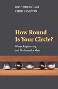
The principal characters in this chapter are two closely related transcendental curves, the tractrix and the catenary, with a strong supporting role being played by a conic section, the parabola. The ways in which the curves are formed are described by the Latin roots of their names: tractare, to pull or draw, and catena, a chain. The tractrix can be demonstrated most conveniently by pulling a weight across a horizontal table by means of a thread. The only way thread can exert any force on the weight is by traction, and in figure 7.1 if the weight starts from A0 and the length of the thread is a, we can see that it can only be moved in a direction directly towards the ‘tractor’ travelling along what we might as well take to be the x-axis.
Its path is a tractrix, with the x-axis as asymptote. The tractor could just as well have moved in the opposite direction, hence the curve is symmetrical about the y-axis, and a tangent from the curve to the x-axis is of constant length. The following derivation of the Cartesian equation refers to figure 7.2. For future reference, note that y/ sin (t) = a, and so is constant.
The length of PB (the tangent) is a, and applying the Pythagorean theorem to the triangle PBC we have ![]() and therefore
and therefore

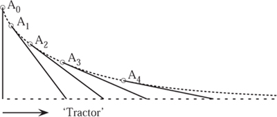
Figure 7.1. Pulling a weight with a thread.

Figure 7.2. Half of the tractrix.
or
This is a standard integral giving
![]()
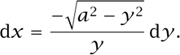
The solid of rotation about the asymptote is known as a pseudosphere. A model of half of this solid is shown in figure 7.2. The work done by friction on some small area A is proportional to Al sin (t). In fact, the work against friction is proportional to Al2πy per revolution, where the coefficient of friction and the axial loading are assumed to be constant. Therefore, to obtain our even-wearing bearing we require y to be proportional to sin(t), and, as we have already seen, this is true of the tractrix. In practice it is difficult to machine both male and female components of a bearing to be tractrices. Schiele approximated the curve by two straight lines producing a two-cone bearing. Notice the discontinuity between the angles to allow for easier grinding and polishing: the same technique was mentioned earlier with the vee-blocks. Both the thrust bearing and Schiele’s bearing are shown in figure 7.3.
Figure 7.3. (a) The thrust bearing and (b) Schiele’s bearing.

Figure 7.4. A tractrix as an orthogonal trajectory through a set of circles.
Returning to figure 7.2, it is clear that a circle of radius a centred at B cuts the curve orthogonally—this provides an alternative way of describing a tractrix as the orthogonal trajectory through a set of circles where the centres lie on a straight line. The axis itself is also an orthogonal trajectory. This suggests another way of drawing a tractrix. The more closely the circles are spaced the more closely the short straight-line segments will approximate to the true curve (see figure 7.4). Larger and more general tractrices are described by the path of the rear wheel when a bicycle is steered in different directions, and the same can be seen when a stretch limousine or long articulated lorry takes a sharp turn. The final example we give is of a lethargic dog being taken for a walk on the end of a long straight chain. This is just the same as pulling a weight if the dog walks slowly and the lead is always under slight tension. However, if you stop and the dog approaches you, the lead will slacken and form the next curve we describe: a catenary.
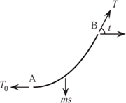
Figure 7.5. Forces on a section of hanging chain.
A catenary is the natural curve taken by a uniform flexible chain acted on only by gravity as it hangs between two supports. Its equation can be found by looking at half of the chain (see figure 7.5). Here, A is the midpoint of the curve, its lowest point, where the tension is T0. At some other point B on the curve, the tension is T, making an angle t with the horizontal. We assume that the mass of the chain is m per unit length, and the arc length from A to B is s. We can now resolve forces:
T0 = T cos(t) and ms = T sin (t),
giving
![]()
Define a = T0/m so that s = a tan(t). This is the intrinsic equation of the catenary, being independent of any coordinate axes. For our purposes, though, it is more convenient to be able to write it in the more common and applicable form of the Cartesian equation in x and y :
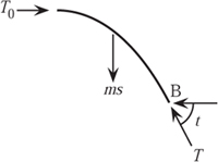
Figure 7.6. Forces on a section of an arch.

Figure 7.7. A suspension bridge.
![]()
and
![]()
These expressions may be integrated to give
x = a ln (tan ![]() π +
π + ![]() t)),
t)),
y = a sec (t).
The elimination of t gives
y = a cosh (x/a).
If we turn the diagram upside down to form an arch, the only changes are that what was in tension is now in compression and the directions of both arrows have been reversed. This leads to the conclusion that the inverted catenary is the natural, and best, form for an arch (see figure 7.6).
The main cables in a suspension bridge hang in a catenary, certainly before any decking is added, and this extra load has very little effect on its shape. In the crude sketch of figure 7.7 the two towers are being pulled towards each other because of the unbalanced loading. The obvious solution, seen in virtually all suspension bridges, is to extend the cables over the top of the towers to massive anchorages at the ends of the approach roads. This is possible only if the approach and centre spans lie in a straight line. This solution was not available to Isambard Kingdom Brunel when designing the Royal Albert Bridge to cross the River Tamar at Saltash. The lie of the land is such that the approaches to the main spans over the river had to be sharply curved, making it impossible to construct a conventional suspension bridge. The elegant solution he proposed, and built, was to use the catenary in two ways. One half of the load of the rail deck was suspended by chains, as in a suspension bridge, while the other half of the load was suspended from a beam in the form of an inverted catenary. In this way the loading of the three towers of the two main spans of the bridge was balanced so that no staying cables were needed. This is shown in figure 7.8.

Figure 7.8. Brunel’s Royal Albert Bridge across the River Tamar at Saltash.
Returning now to the geometry of the curve, we consider the evolute, which is the locus of the centres of curvature. The evolute of the tractrix is the catenary. This is shown in figure 7.9. AB is a tangent to the tractrix at B and CB is a normal to it whose length equals the radius of curvature at B. The locus of C describes a catenary. In fact, there is no need to know the radius of curvature as CB is a tangent at C so a series of normals will define the envelope of the same catenary. In the same way, the tractrix is the evolute of a catenary.

Figure 7.9. A catenary as the evolute of a tractrix.
We can now introduce the parabola—an algebraic curve—and show how it is related to a catenary. The first point to note is that near their vertices the curves are indistinguishable. As we have already seen, a catenary is the curve taken by a uniform flexible chain, so its loading is constant per unit length of arc. A parabolic curve results when the loading is constant per unit horizontal length.
In order to show that this is true we can repeat the analysis already used to derive the equation of the catenary with only a few small but significant changes. The principal change is that the curve has been drawn on Cartesian axes, and the loading is now m per unit horizontal length; tan(t) can be written dy/d x. After resolving forces,
![]()
Assuming that the curve passes through the origin, a solution is y = x2 /4 a, for a suitable choice of constant a. This curve is a parabola.
In a suspension bridge where neither the weight of the cable nor that of the decking can be neglected, the actual curve must be somewhere in between. The fact that the curves are very similar, almost indistinguishable, near their vertices is due to the fact that they are tangential to the horizontal. Here, the ratio between uniform horizontal loading and uniform loading per unit length is proportional to the cosine of a small angle, which is extremely close to one.
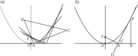
Figure 7.10. Generating a parabola from an envelope of lines.
A more fundamental relation between the two curves is that the locus of the focus of a parabola rolled along a straight edge is a catenary. This may appear strange at first sight because one is an algebraic curve while the other is transcendental. The link arises because the expression for the arc length of a parabola is given by a transcendental function: the logarithm. In order to simplify what follows we look first at a parabola. One way of drawing this curve, or rather its envelope, is shown in figure 7.10(a).
Take a straight edge and fix this to a drawing board and place a pin, F, a distance a above the edge to act as the focus of the parabola. As the 90° corner of a square is moved along the edge with side AB resting against the pin, AC is tangent to the parabola. For the purposes of cutting out a template an envelope is just as easy to work to as a single line obtained from plotting the curve.
While you have a straight edge and pin to hand a brief digression is permissible. What would happen if you used, say, the 30° or 60° corner of the square instead of the 90° corner? If the straight edge is replaced by a line, and the square by a template of an angle greater that 90°, what is the outcome? Defining curves as the envelope of a family of lines provides some very interesting and enjoyable problems. You can also make some curves yourself with card and thread, and these can make very interesting decorative patterns. We shall again make extensive use of curves defined as the envelope of a family of lines in section 10.9.
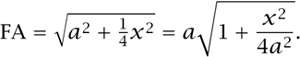
In figure 7.10(b) the parabola x2 = 4ay is shown with the tangent from P, which cuts the x-axis at A, and where PN is drawn perpendicular to the x-axis. With the focus at F, join F and A. By definition, angle FAP equals 90°. In the triangle PNA we have
![]()
and hence AN = ![]() x. Therefore, OA =
x. Therefore, OA = ![]() x and so
x and so

In the triangle FOA we have
Another way of looking at the diagram is that the parabola is stationary and the straight edge has rolled round until P is the point of contact. The origin O has now moved to a new position O′. The length of FA is then the new y-coordinate of the focus, say Y. The length of O′P must be equal to arc length OP. Calculating this arc length is a rather lengthy calculation, which we have chosen to omit since it adds little to our story. It is quite standard and can be found in many calculus books such as Maxwell (1954, volume II, p. 105). The result we need is that

Given that X = O′P - PA we have that
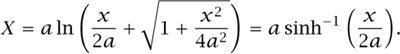
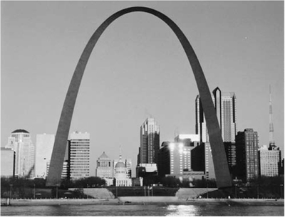
Figure 7.11. Jefferson National Expansion Memorial. Photo courtesy of the National Park Service, Jefferson National Expansion Memorial.
Or sinh (X/a) = x/2 a and
![]()
therefore e X/a = (x/2 a) + (Y/a). From this we have
![]()
which proves the relationship between the two curves.
The grand finale to this chapter is a catenary arch, the Gateway Arch, a striking part of the Jefferson National Expansion Memorial at St Louis, Missouri, in the United States. This stainless steel monument stands 630 feet high and is 630 feet wide at ground level. Its cross-section is that of an equilateral triangle whose side length tapers from 54 feet at the base to 17 feet at the top, where there is an observation room.
The form of the arch is defined by
![]()
This is not the equation of any curve seen by just looking at the arch, e.g. the outside boundary seen in figure 7.11. It is the more important equation defining the locus of the centre of gravity of the cross-sections of the tower. The derivation of the equation of a catenary given earlier in the chapter assumed a constant mass per length of curve, although this is certainly not the case with this arch.