Chapter 3
FOUR-BAR VARIATIONS
It is quite conceivable that the whole universe may constitute one great linkage, that is, a system of points bound to maintain invariable distances, certain of them from certain others, and that the law of gravitation and similar physical rules for reading off natural phenomena may be the consequences of this condition of things. If the Cosmic linkage is of the kind I have called complete, then determinism is the law of Nature; but, if there be more than one degree of liberty in the system, there will be room reserved for the play of free-will.
Sylvester (1875b)
Linkages are such an important topic that we cannot restrict our attention solely to drawing a straight line. The simplest linkage mechanism contains only three obvious bars, and a fourth if you count the fixed base. These found an application in generating an approximate straight line. Of course, applications of four-bar variations are not restricted to generation of approximate straight lines. We shall examine these linkages in more detail and consider the curves that four-bar linkages actually generate.
It is not possible to attempt to list all the other uses here, so instead we shall take a small sample for the purposes of illustration and suggest that you look around to see how often they are used. Sometimes they are not obviously linkages, as one or more of the links may form part of the whole structure, but nevertheless they are there. Look at pushchairs, long-handle loppers for pruning trees and much of the machinery used on large building sites. Indeed the modern area of robotics relies heavily on linkages and while we have concentrated here on some historical uses, this is a field which is very much alive.

Figure 3.1. Four bars in the form of a parallelogram.
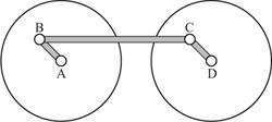
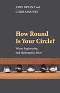
Figure 3.2. The coupling rod of a steam engine.
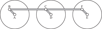
Figure 3.3. Coupling six wheels of a locomotive.
As a general comment on all linkages, and we can take Watt’s as an example, it may not always be apparent that the fixed link AD is itself a link. These fixed pivots could be on a base board as in figure 2.6, or fixed to the engine house of a beam engine, or on the frame of the engine itself. Nevertheless, they act as links. We start with a parallelogram where AD = BC and AB = CD (see figure 3.1). The parallel rule used for navigation is a clear example because each member looks like a link. AD and BC are the rules and the shorter sides are plainly links. The word ‘parallel’ in this context signifies that the outer edges of the rules remain parallel however widely the rule is opened. This contrasts with the same word being used by early engineers to signify movement along straight parallel lines some prescribed distance apart.
A far less obvious linkage could be seen almost anywhere on the United Kingdom’s steam railway system until the early 1960s, and may still be seen on preserved locomotives. It is the coupling rod used to transmit power from the driven axle to other axles to improve the performance of the locomotive. The coupling rod is the one element of the parallelogram which looks like a link; the other longer link is the frame of the locomotive itself, and AB and CD are parts of the hubs of the driving wheels. Figure 3.2 shows a ‘four coupled’ locomotive, and, as an aside, the coupling rods on each side of a locomotive would normally be 90° out of phase to avoid problems when starting on dead centres, i.e. when A, B, C and D lie in a straight line. It was common to have six coupled wheels on locomotives and power was transmitted by two parallelograms joined end to end as shown in figure 3.3. So far it has been possible to designate one or two of the pivots as being fixed, and in this instance the fixed points are obviously the axles A, D and E. However, this is not actually practicable as all axles are sprung, giving each axle some degree of vertical movement to allow for imperfections in the track. This implies that BCF cannot be a single link with pivot holes at B, C and F, as it would then be subjected to bending stresses. Instead the rod is made of two sections, often sharing a pivot at C.
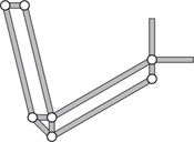
Figure 3.4. Parallelograms used on a drawing board.
Two parallelograms can be joined in a slightly different way to form a linkage commonly used on drawing boards. Two rules were joined to make an L-shape, the purpose of the linkage being to allow this form of square to be moved over the board preserving its orientation, so the horizontal leg is always parallel to the base of the board with the other leg square to it (see figure 3.4). The main difficulty in making a model linkage is deciding how the separate links should be pivoted, and here we offer some suggestions. If you have a fully equipped workshop with a lathe and a vertical mill, you will not need any advice on how to use them to produce a properly engineered metal linkage—but do not dismiss the rest of this section just yet. However you make a linkage, of whatever material, it is always a great help if you start by making a mockup using strips of cardboard, plywood or Meccano. It does not matter how crude it is or how well it works as its purpose is to find how the links should be arranged in the plane so that they do not foul each other unnecessarily. As an example we consider Watt’s linkage, and its more generalized form, where the distance between fixed pivots can be varied. The long arms of the Watt’s linkage in figure 2.6 are designed to move only some 20° either way from their central position, and the links can therefore be positioned as shown in figure 3.5.
Figure 3.5. Links from the side: no fouling.
![]()
Figure 3.6. Links from the side: extra vertical space to avoid fouling.
3.1 Making Linkages
Note the provision of spacers/washers. This arrangement would not be suitable for the general linkage as the long arms would foul each other when the fixed pivots are arranged close together, so a better scheme is shown in figure 3.6.
In any linkage the crossing of individual links cannot be avoided. So in general, it is not possible to draw a complete curve: narrow links are a real advantage. A simple method we have used to make linkages is based on press studs and the wooden sticks or spatulas that are often provided with ice cream or in cafes and coffee bars in place of teaspoons. Press studs are remarkably good pivots as they turn freely, yet they have little play and can easily be glued to the wood with an epoxy resin. They can also be taken apart and the links reused. Haberdashery shops and market stalls offer a wide range of sizes and designs, and the best for our purposes are those with raised centres on the base of the faces. The reason for this is that whenever a centre is marked on a link it is difficult to glue the stud in position accurately. It is better to define the centre with a small hole, say 1.5 mm in diameter, so as to provide a definite location for the stud. It also helps if the hole goes through the wood to provide a definite centre for another pivot or as an aid to further marking out. Glue the studs separately before joining the links. For those linkages where the tracing point is at a pivot point, Peaucellier’s linkage for example, a different technique is needed. The hole in the two links should be just big enough to take the capillary tube nib of a drawing pen, and the links should be held together with a paper clip glued in position. It looks somewhat inelegant, but it works. Photographic mount card is also a very useful material for a base board, and also for triangular sections such as that which occurs in Roberts’s linkage. An example is shown in figure 3.7, which allows Watt’s, Chebyshev’s and Roberts’s linkages to be demonstrated. This requires only two or three wooden sticks, seven press studs and one sheet of card.
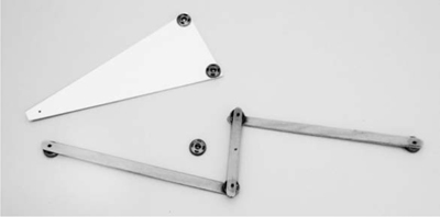
Figure 3.7. A simple model of linkages.
Metal linkages can be made without elaborate workshop facilities by using aluminium strips with pop rivets as the pivots and washers to act as spacers. The idea is to start to tighten the rivets so that the links can turn freely and there is no risk of them separating. Then cut off the wire piece that would usually have come out if the joint had been properly tightened. Care is needed, however, to avoid sharp edges.

Figure 3.8. Forms of the pantograph.
You may have other ideas for easy ways of making linkages—our only comment is that much more is gained by making a model linkage than static sketches.
3.2 The Pantograph
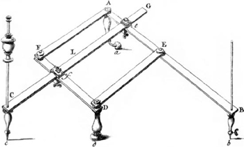
Another important simple linkage is a drawing instrument that is known as the pantograph and is used to enlarge or reduce drawings. Take a careful look at some of the photographs of linkages with engraved brass labels: the one in figure 2.14 for example. The engraving machine used stencils some eight times the size of the lettering and the reduction was achieved by means of a pantograph.
Its simplest form consists of the two rhombi shown on the left of figure 3.8. Imagine the point B fixed to the table. If the point C traces around a shape in the plane, then since ADBE has one-third of the dimensions of BFCG, the point A will trace around an identical shape, one-third the size and upside down. By extending the links AD and FC to intersect at H and then removing points E and G we obtain the usual form of the pantograph shown on the right of figure 3.8. In this new configuration the points all move as before. It is more useful to obtain a copy of a figure which is the same way up as the original. This can be achieved with the linkage shown, where instead of fixing B to the table, A is fixed. Many other configurations are possible, such as that given in Stone (1753), which is reproduced in figure 3.9.
An important application of the pantograph occurs in what is known as an engine indicator. During the nineteenth century and for the first half of the last century reciprocating steam engines were the principal sources of power for ships, locomotives, works and factories of all kinds. It is essential to know how effectively and efficiently the high-pressure steam is being used to generate useful mechanical power, and this is what an indicator does. Its function is to record the pressure of steam in the cylinder at all stages of its stroke and on the return stroke too when the steam is being exhausted from the cylinder. An experienced engineer can see from this when the valve events are taking place—that is to say, when the high-pressure steam valve opens and closes and when the exhaust valve opens and closes, all in relation to the position of the piston in the cylinder.
The first indicator was also an invention of James Watt, and an early schematic is shown in figure 3.10(a). The heart of any indicator is a small cylinder and piston at P, connected to the end of the engine cylinder, closed by a spring-loaded piston. The strength of the spring is chosen to meet the supply pressure of the steam and its piston moves up and down in response to the pressure in the engine. This causes the point R, at which is a pencil, to move up and down. In addition, a string moves the frame horizontally in time with the stroke of the engine. The result is a closed curve that gives the pressure inside the cylinder at any given point of the engine’s cycle. If correctly calibrated, the area enclosed by this curve is directly related to the work done by the engine in a single stroke, and from the stroke rate the indicated power output can readily be found.

Figure 3.10. Steam engine indicators: (a) James Watt’s; (b) Elliott Bros.
In Watt’s indicator above, the pencil is directly connected to the small cylinder. The design of the spring is such that the displacement of the piston is strictly proportional to pressure, and it is this that is recorded on the diagram. The actual movement is often too small to allow a legible diagram to be drawn so it must be magnified, hence the need for the guide linkage. The criteria for this linkage are more exacting than any we have mentioned before. First, the movement of the pencil must always be proportional to the movement of the piston: clearly a criterion not met by a Scott Russell linkage. Second, it must be light, with little friction, because the whole curve is drawn in one stroke of the piston. Many designs were on the market from different makers of indicators and in some, such as that of the Elliott Brothers (figure 3.10(b)), a pantograph was used. Notice the external spring in this design, which is not affected by the high-temperature steam.
So far we have established a linear scale for the pressure axis—the corresponding problem for the stroke axis consists of reducing the displacement over a stroke to a dimension suitable for indicator cards, say around 100 mm. Again, many options were available, the pantograph amongst them.
In addition to its diagnostic uses, such as spotting leaking valves and leakage around the piston, the area of the diagram shows the power developed in the cylinder. From this the mean pressure in the cylinder can be calculated. This leads to the easily remembered formula
power = PLAN,
where
P = mean pressure,
L = length of stroke,
A = area of piston,
N = rotational speed for a single-acting engine (or 2N for a double-acting engine),
all taken in appropriate units.
Indicator diagrams were drawn by their thousands each year when steam engines were the prime movers and this goes to explain why planimeters, the topic of chapter 8, were, and still are, so important.
We would also like to mention here, not so much for its usefulness but for its delightful name, the skew pantigraph (Sylvester 1875b). This can be used for copying drawings with the copy turned through some angle from the original and also rescaled.
3.3 The Crossed Parallelogram
If the parallelogram is crossed, a new range of applications is possible. The Hart inversor already mentioned can form the basis of an exact straight-line linkage. Another application of a crossed parallelogram is in the steering mechanism of a cart. If the front and back wheels are both steerable, and connected by a crossed parallelogram, then the turning circle of the cart is vastly reduced. In fact, the crossed parallelogram has some remarkable properties. The first remarkable property is that in all positions, the angles at A and C (see figure 3.11) are equal, as are the angles at B and D. We shall assume that A and B are fixed and that C and D move. The question to resolve is the path of the hypothetical point P, not marked on the diagram, where the lines AD and BC cross. We note by symmetry that the distances APB and CPD are equal in any position of the configuration and are hence constant. Imagine a piece of string of fixed length from A to P and back to B. The string constrains the position of P—you may be familiar with the string-and-pin method for drawing an ellipse. Indeed, if we view A and B as the foci, then the locus of P will be an ellipse. We shall leave the detailed examination of this topic until section 13.3, where it is compared with a variety of other methods. Notice, however, that it is clear how to find the tangent to the ellipse from this linkage. Although it would be hard to construct a device for drawing an ellipse from this idea, Artobolevsky (1976, volume 2, p. 93) does indeed propose such a linkage. Since C and D can be thought of as being the foci of another identical ellipse, this linkage configuration can be used as the basis for elliptical gears.

Figure 3.11. A crossed parallelogram.
Elliptical gears can be used to produce variation of speed between given limits. This has been used as a quick return motion, for example, and also in pumps, printing presses and other applications in which most of the work is done in one direction and it is important to return to the original position as quickly as possible. However, such mechanisms are not common. Creating circular gears is a difficult and specialist topic in itself, and the difficulty in measuring the perimeter of an ellipse adds to the complexities.
The practical uses of the elliptical gear are endless, and it would be in greater use and favor, if it were not for the fact that its production, by the means ordinarily in use for that purpose, is as difficult and costly as the resulting gear is unsatisfactory.
Grant (1907)
3.4 Four-Bar Linkages
In chapter 2 we looked in detail at four-bar linkages from the point of view of the generation of approximate straight lines. In fact, such linkages produce a variety of interesting curves. One way to see these is to use a model in which the distance between the fixed axes is adjustable. For example, in the models in plate 10 the longer arms are 5 units long and the short middle arm is 2 units long. In the positions shown the curve is close to Watt’s linkage and exactly equal to Chebyshev’s. All the intermediate positions are possible by moving the arms.
Taking an approach using only elementary trigonometry and algebra does not yield a simple description of the path of the point on the linkage—in this section we shall provide a formula. In particular we shall take the four-bar linkage ABCD, where A = (x1,y1), B = (x2,y2), C = (x3,y3) and D = (x4,y4). Simple applications of the Pythagorean theorem arrive at a system of equations such as
(x1 − x2)2 + (y1 − y2)2 = (r1)2,
where r1 is the length of AB.
If we take P = (x, y), and assume that P lies on the line BC, or on an extension of this line, then we arrive at the following weighted average for the position of P on the line BC, for some p1 and p2:
x = p1x2 + p2x3 and y = p1y2 + p2y3.
We then have a system of four quadratic equations and two linear equations. The prospect of solving such a system to obtain the position of P relative to the two fixed points A and D appears to be hopeless. However, with the aid of a modern technique, known as Gröbner bases, it is possible to solve systems such as this exactly. For the purposes of comparison with chapter 2 we shall assume that AB = CD = 5 and that CB = 2. If we assume that P is at the centre of CB, then p1 = p2 = ![]() . However, we shall position A = (−r,0) and D = (r,0), so that for r = 2 we have Chebyshev’s crossed linkage, and for r =
. However, we shall position A = (−r,0) and D = (r,0), so that for r = 2 we have Chebyshev’s crossed linkage, and for r = ![]() ≈ 4.898 we have Watt’s linkage. Solving the resulting systems of equations gives the path of P as
≈ 4.898 we have Watt’s linkage. Solving the resulting systems of equations gives the path of P as
r4(y2 + x2) + 2r2(y4 − 26y2 − x4 + 24x2) + (y2 + x2 − 24)2(y2 + x2) = 0.
Notice that for each particular r this gives not an explicit equation for y in terms of x, but rather an implicit relation between x and y.
If we solve this equation from a purely algebraic point of view, using numerical techniques if necessary, then we see that the curve for Chebyshev’s crossed linkage has two disconnected curves, not just the single portion shown in plate 2. Of course, this is because continuous movement of a mechanism might not allow all parts of the feasible curve to be reached. Usually, whenever we have the intersection of two circles, or a circle and a line, there are two equally valid solutions. Hence, from a mechanical point of view this results in ambiguity as to which solution should be chosen. In a physical mechanism such ambiguity is usually, but perhaps subconsciously, designed out. When it exists it can give rise to very interesting dynamics, an example of which we will examine in section 3.7.

Figure 3.12. The locus of Watt’s linkage for various separations r.
Figure 3.12 shows the variety of curves that can be generated by changing the distances between the fixed pivots shown in plate 10. They range from a point where all the links are in line with AD = 12, via Watt and Chebyshev linkages, to a circle where A and D coincide.
One particularly famous curve is known as the lemniscate of Bernoulli, shown in figure 3.13, which can also be drawn using a crossed parallelogram. If we take
AB = CD = 1,
BC = AD = ![]() ,
,
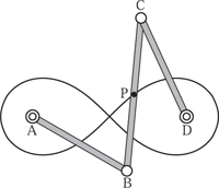
Figure 3.13. The lemniscate of Bernoulli.
with A and B as the fixed points
A = ( − ![]() ,0), B = (
,0), B = (![]() ,0),
,0),
then the path described by P is
(x2 + y2)2 = a2(x2 − y2),
where ![]() is a scale factor. The curve gets its name from the Greek lemniskos, a bandage or ribbon, via Latin.
is a scale factor. The curve gets its name from the Greek lemniskos, a bandage or ribbon, via Latin.
3.5 The Triple Generation Theorem
We conclude our work on four-bar linkages with a most remarkable result known as the triple generation theorem. You may recall that in section 2.1 we found two arrangements of linkages that resulted in one path for the point P. In this section we find three linkages that all result in generating the same path. It is deceptively simple to do this, and to start we draw an arbitrary triangle ABC and select any internal point P. If we draw lines through P parallel to the sides of ABC then we can create the three general four-bar mechanisms shown in figure 3.14. Here, just as with Roberts’s approximate-straight-line mechanism, the point P does not lie on the middle linkage.
Now, if we fix pivots A and B closer together to allow the point P to move, then C remains in one place as P moves. Alternatively, the three general four-bar mechanisms each constrain P to move along the same locus.

Figure 3.14. The triple generation theorem.
The mathematician will probably be wondering if an arrangement of linkages can be found which will generate any given curve. A paper by Kempe (1876) showed that for any algebraic curve there exists a linkwork which will generate it. The original paper is somewhat condensed and Yates (1949), who works up to this result through some 200 pages of carefully structured exercises on the subject, is probably more enjoyable to read.
3.6 How to Draw a Big Circle
It might seem strange to consider here how to draw a circle, since a rudimentary pair of compasses can be fashioned from almost any rigid object. However, drawing the arc of a circle with a very large radius is quite problematic in practice. Not only will the centre be a long way away, but constructing and moving a large rigid object is never easy. Draftsmen used a collection of template arcs of prescribed radii, known as railway curves. Although this is a practical solution when the radii are known, it is unsatisfactorily restrictive. While in chapter 1 we suggested constraining a wedge between two pins, this is hardly going to provide a technique sufficiently accurate for engineering purposes. Furthermore, in keeping with the rest of this chapter we would prefer to use rigid linkwork to constrain the motion.
Perhaps it is not surprising that Watt’s linkage can generate an approximate circular arc of large radius, and indeed this arrangement has been applied to cutting and polishing large stone blocks by Keady, Scales and Fitz-Gerald (2000). However, Peaucellier’s cell, which gave an exact straight-line motion, can easily be adapted to generate an exact circular arc of very large radius. The resulting device is compact and it is not necessary to be able to physically get to the centre of the circle.
To see why this is the case, we recall the fundamental relationship between the points O, C and P in figure 2.16. Peaucellier’s cell is an inversor, which is to say that OC • OP = k2. We shall forget temporarily about linkages and just concentrate on this mathematical relationship between points in the plane. We shall assume that a point C is a distance r from the origin and that the line OC makes an angle t with the horizontal. Then the point P is a distance k2/r from the origin, and OP is also at an angle t with the horizontal. The relation OP = k2/OC gives rise to the description of P as the inversion of C in the circle of radius k.
In general, if point C moves along a line through the origin, then the angle remains constant. Hence P will also move along the same line. If C moves along a circle through the origin, as we have already seen, P moves along a straight line. Conversely, if C moves along a straight line, P follows a circular arc, which is part of a circle through the origin. This might allow us to draw arcs of large circles, but we have already seen that constraining a point to move in a straight line is problematic. The last case is when C moves on a circle not through the origin. Here P also moves along a circle. Proving these statements using elementary trigonometry is not a pleasant task—a much more aesthetically appealing approach requires the slightly more sophisticated machinery of complex analysis, which we choose not to examine in detail in this book. See instead the elegant book of Needham (1997).
For us, if we change the length of the distance OQ in figure 2.16, then the circle on which C is constrained to move will no longer pass through O. As a result P will now move along a circular arc, and it is the radius and centre of this we now find using elementary methods. Notice at the top of plate 4 that the additional holes allow exactly this situation to be illustrated. We shall not find the extent of the circular arc which a configuration of linkages can generate. Although this is possible, the resulting formulae are not particularly enlightening.
We appeal to symmetry to argue that the centre of the circle along which P moves must lie on the x-axis. Although the inverse of the centre of the circle does not correspond with the centre of the inverted circle, we can find the centre by taking the average of two points on a diameter. Adopting the same notation as in figure 2.16, we now assume that OQ = l3 and QC = l4, where now it is no longer the case that all these links are of equal length. Assuming that P moves on a circle with centre at centre R = (l5,0) and radius l6 we have the two potential situations. The first assumes that l3 > l4, shown at the top of figure 3.15, and the second assumes that l4 > l3, shown at the bottom of the figure.
For the case in which l3 > l4 we have that
![]()
Solving these equations gives
![]()
The case in which l3 < l4 is very similar.
Notice that if l3 and l4 are very similar then the radius, l6, is very large indeed and the centre correspondingly far away. If l3 = l4 then we would need to divide by zero, giving an infinite radius, which is forbidden. In this case we already know that we have a straight line, although we shall again appeal to the fiction that a straight line is a circle of infinite radius in section 8.5.
3.7 Chebyshev’s Paradoxical Mechanism
We end this chapter with a most intriguing and remarkable mechanism which Artobolevsky (1976, section 601) describes as Chebyshev’s paradoxical mechanism. A model of this mechanism is shown in plate 11. It is described as ‘paradoxical’ since one revolution of the crank handle corresponds to two revolutions of the flywheel in the same direction, or to four revolutions in the opposite direction. This mechanism really is worth constructing, if only to confound your friends and colleagues. A schematic of the mechanism is shown in figure 3.16.

Figure 3.15. Using Peaucellier’s linkage to draw a large circle.
The lengths of the linkages must satisfy
AB = CB = MB = 1,
FC = 1.387, EA = 0.557, DM = 0.584,
CE = 1.324, FD = 0.123.

Figure 3.16. Schematic of Chebyshev’s six-bar paradoxical mechanism.
Furthermore, the angle FCE, shown as a dotted line in the diagram, must be a right angle. The crank handle is at A, and the flywheel is pivoted at F. In this diagram, the links BC, AE and AM form a four-bar linkage, which is very similar to the alternative form of Chebyshev’s approximate-straight-line motion shown in figure 2.12. The locus of the point M as the point A is moved around a circle is shown as a dashed line in the diagram.
There are two other links to complete Chebyshev’s paradoxical mechanism: these join F to a point D, and D to M. These are shown as lines, rather than links, in the diagram. Since the position of the point D is given as the intersection of two circles, one centred at F of radius FD = 0.123 and one centred at M of radius DM = 0.584, there are two choices for the position of the point D, shown as D1 and D2 on the diagram. It is precisely the ambiguity between these two choices that gives rise to the apparently paradoxical behaviour of the flywheel at F when A is rotated.
What is so unusual in this mechanism is the ability of the linkages to flip from one configuration to the other. In most linkage mechanisms such ambiguity is implicitly, or explicitly, designed out so that only one choice for the mathematical solution can give a physical configuration.