Chapter 13

FINDING SOME EQUILIBRIUM

If you throw a silver dollar down upon the ground, it will roll because it’s round.

Attributed to Jack Palmer and Clarke van Ness (1939)

 

 

The words of the song are true enough though eventually the coin will lose its rotational energy, fall to one side and stop. It rolls, as does any circular disc, cylinder or ball, because its centre of gravity remains a constant height above a horizontal surface independent of position.

Following on from the last chapter, which was all about balance, we consider a number of related rolling problems. The first involves two joined cones which appear to roll up a slope. Secondly we show a way of joining two identical discs so that they will roll with no preferred position. We then do something similar for ellipses, before finishing with a solid model based on a generalized ellipse, known as the ‘super-egg’.

13.1 Rolling Uphill

We shall begin with an experiment involving two rolling cones. Cones are a basic shape in solid geometry with which we hope you are familiar. Figure 13.1 shows two cones joined at their bases. The experiment is conducted by resting the cones on supports at the bottom of a slope. However, these supports are not parallel, and they can be arranged in such a way that when released, the roller appears to move uphill. The reason for this is simple. As the supports on which the roller rests are not parallel, the centre of mass of the cones actually descends, although the position on which the roller rests does rise. This illustrates an important principle: centre of mass will move downwards whenever possible.

Figure 13.1. A roller that moves up a slope.

Figure 13.1 is taken from Leybourn (1694), in which the author claims that the rollers are a novel invention. There are various ways to make a modern version. Two traffic cones together with scaffold planks make a slightly larger and equally compelling practical experiment.

The uphill roller is a three-dimensional problem, so in order to describe it we need to sketch the situation carefully. This has been done from three perspectives in figure 13.2. We take the origin O to be where the two support lines meet, the angles these support lines make with the horizontal as t and with each other as 2s. The centre of mass of the double cone, which has coordinates x and y, is labelled G, and the cones have a base radius of r and a height of h. From this it is clear in the end view that tan(u) = r/h. There is a natural symmetry in the problem, so that we only mark one point of contact of the cone with its support, which we call A.

Our task is to describe the height y in terms of x, and hence derive criteria for y to decrease as x increases—so that G goes down even if A goes up.

Figure 13.2. A sketch of the uphill roller.

From the plan view we have that

q = x tan(s).

From the end view,

BC = q tan(u) = x tan(s) tan(u).

Using the front and end views we have that

y = AD + CG

= AD + BG − BC

= x tan(t) + r − x tan(s) tan(u)

= r + x(tan(t) − tan(s) tan(u)).

From this it is clear that if tan(t) – tan(s) tan(u) = tan(t) – (r /h) tan(s) is negative, then the roller will move uphill.

13.2 Perpendicular Rolling Discs

Let us continue with another practical experiment in which we take two identical thin, uniform discs. The experiment involves slotting the two identical discs together. The most important thing from a practical point of view is to ensure that the discs are fixed together radially and are perpendicular. We shall assume, for the sake of argument, that the radius of both discs is one unit and we shall ensure that the distance between the centres of the discs is exactly units, which in practice is about 1.414.

You should now have two discs that look like those shown in plate 30. Now try rolling them along a horizontal table surface. They move in an intriguing way and do not seem to have a preference for any one orientation. In fact, in this section we will show that no matter what the orientation of this compound object, the centre of mass is indeed a constant distance from the table. Hence, the shape will roll along the table top without naturally moving towards, or resting in, one particular orientation.

What is particularly striking about the problem is that it is fundamentally three dimensional. Some problems, such as that of stacking dominoes, can easily be reduced to a two-dimensional problem that is much easier to solve. If you try to make these discs and roll them along a flat surface it will soon become apparent that there is a complex three-dimensional motion in play. Furthermore, the object we have made only makes contact with the surface of the table in two places, whereas when we talk about an equilibrium position of a solid on a plane we usually need at least three points of contact. Finally, there are obvious symmetries in the shape and in its motion. All these factors make modelling and describing the motion of this model quite an interesting problem.

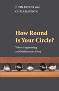
Let us begin by describing the problem in more detail. We have two thin uniform discs of radius 1, called D₁ and D₂, with respective centres O₁ and O₂. These are slotted together along diameters with the centres a distance x apart, and the planes of the discs are perpendicular. We assume that this object rests on a horizontal plane surface. The disc D₁ will touch the table at a point C₁ on its edge. The angle between O₁O₂ and O₁C₁ is called t₁.

By symmetry, the centre of mass of the object lies halfway along the line connecting O₁ and O₂. Our task is to choose x such that, no matter the orientation of the object, the centre of mass lies a constant distance above the surface of the table. Of course, it is by no means obvious that such a choice is possible. Our first task is to consider some simple cases that will help us establish what the value of x might be.

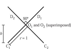
Figure 13.3. End view along O₁ O₂.

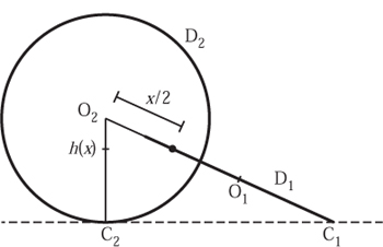
Figure 13.4. Side view when D₂ is vertical.

There are two ‘extreme’ positions for the object. The first occurs when t₁ is 90°, at which, by symmetry, the point of contact of D₂ with the table is also at t₂= 90°. In this configuration the line connecting O₁ and O₂ lies above, but parallel to, the plane of the table itself. Hence x does not affect the height of the centre of mass above the table. In this configuration, looking along the line connecting O₁ and O₂ we see what is shown in figure 13.3.

From this it is clear that h(x), the height of the centre of mass above the table, will be Since this does not depend on x, if h is to be kept constant then it must take this value.

Roll the discs to find the second ‘extreme’ position, which occurs when t₁= 0°, forcing D₂ to lie in a vertical plane. Looking from the side we see what is shown in Figure 13.4.

The distance from O₁ to C₁ is 1, and from O₁ to O₂ is x. Furthermore, the triangle O₂C₂C₁ forms a right-angled triangle. A simple application of similar triangles shows that h(x) is given by the equation

Since we are trying to find a configuration in which the centre of mass lies a constant distance above the table, we are trying to solve

Rearranging this equation to solve for x gives

x =

If the distance between O₁ and O₂ is chosen to be , then the centre of mass will be a distance above the table in both of the extreme positions. Physically, to achieve this we cut a slot 1 times the radius in each disc.

The height of the centre of mass is now guaranteed to be the same in two positions, and more mathematical work using three-dimensional geometry is necessary to determine whether or not this height is totally independent of the position of the discs.

An alternative experimental approach is to get two discs whose thickness is small in relation to their radii and see what happens. Our first trial was with two plastic discs of 20 mm radius and 1 mm thickness, which used to come with packets of potato crisps. They rolled beautifully and provided excellent experimental evidence.

In the elementary geometric analysis of figures 13.3 and 13.4 we assumed that the discs were thin, i.e. that they had no thickness whatsoever. Further thought shows that this need not have been assumed in the first place provided that the rims of the discs are thin: nothing has been assumed about the rest of the discs. In fact, discs of almost any thickness can be used provided the perimeters are chamfered to a knife edge and that they are symmetrical about their centre planes. Figure 13.4 shows that when D₁ is at its closest to being horizontal it makes an angle of to the horizontal: a chamfer at a sharper angle satisfies the condition that, as far as rolling is concerned, the discs are thin.

Figure 13.5. Slotting rings.

Unlike the solids of constant width described in section 10.3, there is some merit in using a dense material to make this model. The extra mass helps the discs roll along smoothly and overcome air resistance as well as providing stronger support around the slots.

The discs need not be complete circles and they make attractive toys. One possibility is to use the rings shown in Figure 13.5, where the inner radius is ( − 1) R.

For the minimalist they need not involve discs or rings at all, just a wire skeleton. Indeed, the outline of the shapes shown in plate 31 is sufficient. This form is difficult to make and to provide with strong joints. It does suggest that we are dealing with the skeleton of a solid the surface of which can be created from a flat sheet without any need to crease or stretch it in any way. The outline, or pattern, can be found mathematically or by experiment. Wipe some lipstick or engineer’s blue round the rims of the model, but only where they touch the surface when rolling otherwise it can be a messy job. Roll the model over a sheet of paper or card and there is the pattern ready to cut out. As with all solid models made from card it is difficult to glue the edges together, but it is worth a try. Failing this, the pattern can be transferred to cloth, making allowances for the hems. With suitable stuffing you can have a soft toy, although now it is hardly a mathematical model!

In the rest of this section we shall return to our mathematical analysis of the rolling discs to show in detail that the height of the centre of mass does indeed remain a constant distance above the table. In the next section we shall do something very similar with two ellipses.

In order to consider the general situation we shall consider the contact point of D₁ with the table: we label this point of contact C₁. We assume that the object is sitting on the table, with D₂ touching at the point, not shown, that we call C₂. Ignoring the symmetry of D₁ and D₂, the position of C₁ is enough to dictate the position of the object uniquely.

To help us consider the position of the point C₁, we shall draw a line through the centre of each of the discs. Note that this line also lies in the plane of the discs. To describe the position of C₁ we measure an angle from the line O₁O₂ to the line O₁C₁ in the plane of D₁, and we refer to this angle as t₁. This situation is shown in Figure 13.6, to which we shall refer in the forthcoming discussion. Note that the point C₂ is not shown, since this will be on the disc D₂, shown as a line in figure 13.6, and its position will depend on the angle t₁. We only need to consider values for angle t₁ that lie between 0° and 90°, since the other situations are dealt with by symmetry.

We wish to mathematically describe the object relative to the table, or equally the table relative to the object. Having obtained our mathematical description, we will use this to show that the distance of the centre of mass of the object from the table is constant, regardless of the angle t₁, and hence the position of the point of contact, C₁.

One way to describe a plane mathematically is to specify three points in space. However, we only have two points of contact, C₁and C₂, with the plane of the table—insufficient to describe the plane of the table. Another way to describe a plane is to find a line in the plane and another point that is not on that line. To use this second idea we need to take advantage of the following observation: the tangent line to D₁ at the point C₁ lies in the plane of the table. This line is labelled in figure 13.6 as l₁.

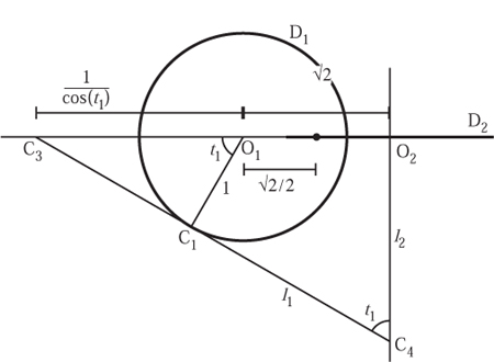
Figure 13.6. Looking in the plane of disc D₁.

By considering right-angled triangles we can also see immediately that the distance from O₁ to C₃ is 1/ cos(t₁). Note that since l₁ lies in the plane of the table, C₃ is the intersection of the line joining the centres of the discs and the plane of the table itself.

The next line we consider is that perpendicular to the plane of D₂ through the centre of D₂. We have labelled this line l₂. Since this line is also in the plane of D₁, it intersects the table where l₁and l₂ meet, a point we label as C₄. Again, simple considerations show that l₁ and l₂ intersect at an angle of t₁, and furthermore that the distance from C₄ to O₂ is given by

Note that we have already considered the case when t₁= 0°, in which l₁ and l₂ do not intersect.

Next we have to consider a different plane altogether: that which is defined by the three points O₂, C₂ and C₄. By considering these, we take account of the line l₁ and the point C₂, and these are sufficient to describe the plane of the table. These form a right-angled triangle at O₂, and since the line tangent to C₂ also lies in the plane of the table, the plane containing O₂, C₂ and C₄ is perpendicular to the table itself. Hence we can use this triangle to find the height,h₂, of O₂ from the table, as indicated by Figure 13.7.

Figure 13.7. O₂ C₄ is perpendicular to D₂;
C₂ C₄ lies in the plane of the table.

In part (a) of the figure we have the general situation. By considering similar triangles, and the Pythagorean theorem, we can easily calculate

Applying this to the situation we need to consider, shown in part (b), allows us to calculate h₂ using the length obtained above for the line C₄O₂. Note that a lengthy, but routine, calculation has been omitted here before we obtain

Thus we are almost there, but actually we did not want h₂ but the height of the centre of mass from the table. To calculate this we consider a third plane. This is a vertical plane passing through O₁ and O₂. We already have a number of points in this plane in our previous diagrams, and combining this information we arrive at Figure 13.8.

We are trying to find h, which is easily calculated as the average of h₁ and h₂. Again using similar triangles we see that

Figure 13.8. Calculating h, given t₁.

and so

The last equality shows that h₁ + h₂ does not depend on t₁ after all, and that the value of h is constant at , as claimed.

13.3 Ellipses

Although the above construction was actually very simple, the calculations provided which show that the construction really worked were quite involved. However, we can actually make this construction more general still and slot together identical ellipses in a similar fashion. Just as the word ‘circle’ refers to the boundary of a disc, so strictly speaking we need planar shapes with elliptical boundaries—we simply refer to them as ‘ellipses’ since the abuse should cause no confusion. Look ahead to plate 32 in which models are shown. However, before we can make such a model we will need to cut out ellipses. In light of section 1.4, some of you may be wondering how this can actually be done. One method, using an arrangement of linkages that assembles some of the components we have already described in chapter 2, is given by Yates (1938). Our goal is more modest, and we will be satisfied if we can draw an ellipse. Hence, we will remind you of some relevant properties of the ellipse and in doing so we will explain how to draw them.

An ellipse is generated by taking a slice through a cone in such a way that we produce a closed curve, much like a squashed circle. The usual form of the equation for an ellipse is

where a and b are positive constants. If b equals a then (13.1) simply reduces to x² + y² = a², which is the equation of the circle. It is a usual convention to assume that a > b and then refer to the longer axis as the major axis and the shorter as the minor axis. Two other points of importance on the ellipse are known as the foci. These lie on the major axis at the coordinates . While this looks complicated, actually locating the foci is simple in practice. Open compasses to half the length of the major axis. Place them on the intersection of the minor axis and the ellipse. The points at which these lines intersect with the major axis are the foci, which we shall refer to as points F and F´.

The foci are the key to many of the interesting properties of the ellipse, which we shall summarize now. Let us take any point P on the ellipse. Imagine a line from F to P and back to F´. This is shown in figure 13.9. The first important property is that the length of the line FPF´ is independent of the position of P. This gives us a first method of drawing an ellipse. Take two pins, a loop of string and a pencil. Place the two pins at the foci and keeping the string under constant tension we can draw an ellipse with the end of the pencil. This is actually rather hard to do, since the string slips off the pencil and the inevitable elasticity in the string causes observable errors. Even if the method could be perfected from a practical point of view, those who have followed chapter 1 should be suspicious since the pencil and pins have circular and not necessarily identical cross-section diameters and the string is broad. Hence we are not really at the foci, and are not really following the centre of the piece of string. If the string is inelastic, and the pins and pen have identical diameters, then in fact a true ellipse is drawn. But since the method is so frustrating anyway we shall not examine any theoretical errors that arise.

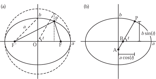
Figure 13.9. Important properties of an ellipse.

The next interesting property is that the normal to the ellipse at the point P is the bisector of the angle FPF´. This means, from a physical point of view, that an elliptical mirror will reflect light emitted from one focus back to the other—hence the origin of the term, perhaps. One way to find the tangent to the ellipse is to construct a line perpendicular to the normal. We take a more direct approach to give the explicit equation for the line tangent to the ellipse at the point (x´, y´). Since (13.1) holds, we have the gradient given using calculus as

From this it is possible to calculate that the tangent line at (x, y) is

Although this does not look much like the equation of a straight line, compare this with (10.1).

Another characterization of the ellipse is to take a parameter t to be any real number and consider (x, y) defined to be

Substituting these values for x and y into the left-hand side of (13.1) reduces to

cos² (t) + sin² (t),

which equals 1 by the Pythagorean theorem. That is to say, the points given by (13.3) all lie on the ellipse (13.1). A circle of radius a drawn around the ellipse is often called the auxiliary circle. The parameter t is then the angle shown in Figure 13.9 and is not the angle between OP and the major axis.

A second practical method for drawing an ellipse is sometimes referred to as the trammel of Archimedes. Take a line AP of length a and mark on the position B so that PB = b. Then constrain this line to move so that A is on the y-axis and B is on the x-axis. From Figure 13.10(a) to move in a vertical straight line. In this ellipsograph only half an ellipse can be drawn at once, and the device must be spun on its pointer to complete the curve. However, there is no trammel to obstruct the curve, making smaller ellipses a practical proposition. We have seen one alternative batch of Omicron model 17 ellipsographs in which the short straight guide in the Scott Russell linkage has been replaced by a single link. This is in fact exactly the grasshopper mechanism we already described in section 2.4. However, now the point A does not move on a straight line but on an arc of a large circle. As a result the path of the pencil is not a true ellipse but only an approximate ellipse.

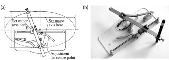
Figure 13.10. The Omicron model 17 ellipsograph.

13.4 Slotted Ellipses

Ellipses can be used in place of circular discs and, if positioned correctly, these roll equally well. Take two copies of the ellipse described by (13.1), and slot them together along the x-axis. If we repeat the analysis we undertook for the discs, then it is clear that the centre of mass will be a distance b above the table, regardless of the distance x. In the other extreme position an analogous analysis involving the tangent to the ellipse given by (13.2) can be used to show that the only possible value of x that also gives this result is

We have omitted details of these calculations and those that prove that using this configuration the height is maintained in all orientations of the ellipses.

Notice that we have not assumed that the x-axis is the major axis, although implicit in (13.4) is the assumption that

If a > b, so that the x-axis is the major axis, then this is satisfied. However, one particularly interesting case occurs when x = 0, which is to say when there is no displacement between the centres of the ellipses. This corresponds to b = a, and a model of this is shown at the top of plate 32. It exhibits a most intriguing rolling action that static pictures cannot hope to capture.

Its behaviour might have been expected though, since any slice through a circular cylinder is elliptical and the cylinder itself can roll. The particular ratio of a to b is such that the ellipses can be slotted together at right angles, and consequently rolling in two perpendicular directions is possible. The geometry is quite different from that of the previous examples, where the ability to roll smoothly was not so easily predicted.

The plywood models in plate 32 were made with b = 0.8 to give a reasonable depth of slot for each model. The most difficult part of making the models is cutting the slots. A saw is the obvious tool to use and the way the elliptical discs were made was to cut the slots first and then paste over a photocopy of the ellipses and finally finish to this shape. It is not worth expending effort and time cutting out two ellipses before slotting because success then depends entirely on the simple saw cuts in each disc. Start with wood that is slightly oversize, cut the slots overdeep and then, holding the wood to the light, paste on the patterns. This works well and rounding the edges improves the rolling performance.

13.5 The Super-Egg

We shall end this chapter with one last gravity-defying model. This is a direct generalization of the ellipse, where we have taken not the equation (13.1) but rather a generalization

where n > 2. To make an ‘egg’ rather than a flat object we shall form a solid of revolution about the vertical axis. That is to say, using the y-axis as an axle we rotate the egg out of the x, y- plane. For the ellipse this solid is known as an ellipsoid and when (13.5) is used we refer to the solid as a super-egg. To illustrate this discussion we take n = 2.5, a = 1 and b = 2. The points with y > 0 that satisfy (13.5) are plotted as a solid line together with an ellipse, as a dashed line, for comparison in Figure 13.11. Hardwood models of the corresponding super-egg are shown in plate 33. The larger egg to the left is made from the wood of the tulip tree, Liriodendron.

Figure 13.11. A super-egg.

For the purposes of our analysis we shall exploit this axis of symmetry, so it will be sufficient to consider the cross-section in only two dimensions.

Imagine placing an ellipse (or ellipsoid) on a horizontal table with the major axis also horizontal. It is intuitively clear that if the ellipse is tipped from this position then the centre of mass will rise, so this position is stable. Similarly, if the ellipse is moved so that the minor axis is now horizontal, then in theory at least there is a point of equilibrium. This will be unstable in the sense that any displacement, however small, will move the centre of mass closer to the table.

We can formalize this by applying the Pythagorean theorem to points that satisfy (13.1). It is easy to see that if r is the distance of the points from the origin then

Initially, if we have the resulting ellipse resting on the horizontal plane y =−b, then whether r increases or decreases for small x is determined by whether b/a > 1, which is equivalent to whether b > a. If a > b, which is the usual situation, then we have the major axis horizontal. It follows that (1 − (b²/a²)) > 0 and so r increases with x. The centre of mass is lifted, so the position is stable. Conversely, if b > a, then we have the minor axis horizontal and it follows that (1 − (b²/a²)) < 0 and so r decreases with x. The centre of mass falls giving an unstable equilibrium.

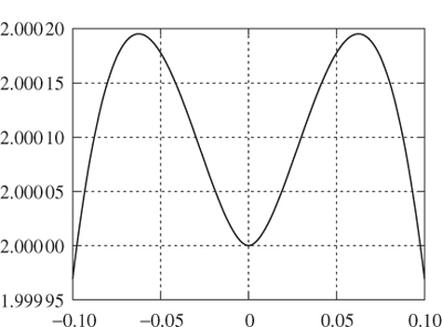
Figure 13.12. The distance from points on (13.5) to the origin for n = 2.5,a = 1,b = 2.

What about the super-egg? If we apply the Pythagorean theorem one last time to points that satisfy (13.5), then we are left to consider

The only case of interest is when b > a, and here it can be shown in general that the centre of mass rises initially. We shall give one numerical example with n = 2.5, a = 1 and b = 2. In this we have taken points (x, y) on (13.5) and plotted the distance from the origin against the x-coordinate for small values of x in Figure 13.12. Notice the exaggerated vertical axis, which indicates that the distance from the origin hardly changes at all, but more importantly it is clear that initially the distance increases. If the egg is displaced slightly from the upright position when the point of contact with the table is x = 0, then the centre of mass will fall by moving back towards this equilibrium. This well of stability allows the super-egg to apparently defy gravity by standing on its end.

Although an explanation of the result is beyond the scope of this book, try this final experiment. With your super-egg lying with its major axis horizontal on a flat table give it a good spin and watch its behaviour very carefully.