Chapter 8

IN PURSUIT OF COAT-HANGERS

Mathematical Instruments are the means by which those Sciences are rendered useful in the Affairs of Life. By their assistance it is that subtle and abstract Speculation is reduced to Act. They connect as it were, the Theory to Practice, and turn what was bare Contemplation, to the most substantial Uses.

Stone (1753)

 

 

In previous chapters we have examined how to draw a straight line and the problems concerned with marking a ruler. In each case we discovered some subtle features associated with these simple ideas. Now we turn our attention to the problem of ascertaining the area of a plane shape.

Area can certainly be measured with complex scientific instruments, such as those shown in figure 8.19 or in figure 8.25. Seeing the undoubted precision involved in their manufacture it may come as a surprise that we are able to begin this description of a hatchet planimeter with details of how to make one. Furthermore, the required raw materials and tools are found in most homes and there is no need for the facilities of a fully equipped workshop.

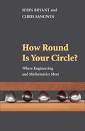
Start with a metal coat-hanger, although any soft wire will do equally well. Cut off a length of about 200–300 mm. Flatten one end to form the hatchet, taking care all the time to keep it symmetrical. A hammer and something to serve as an anvil are all that you need. Clean it up with a smooth file to give a nicely rounded knife blade. This should not be sharp enough to cut anything. The other end is filed to a blunted point with a smooth tip that will not scratch paper. Now bend this into the form shown so that the whole lies flat in a plane and the knife edge is in line with the point. The easiest way to check this is to draw the point along a straight line and see if the knife edge deviates from it. The direction of the knife blade can be tweaked using pliers if necessary. The length of the horizontal distance, marked l in figure 8.1, does not matter, but you will need to know what it is. A ruler is suffciently accurate to measure this to the nearest millimetre, and 100 mm is a good length to aim for.

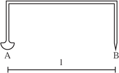
Figure 8.1. A simple hatchet planimeter.

The last job is to glue (or tape) a couple of washers or a nut and a bolt or even obsolete coins above the blade at A. This is not shown in figure 8.1 but is in figure 8.2. This adds a little mass above the knife blade and makes the device much easier to use in practice—the weight need not exceed 200 g.

You have made a hatchet planimeter and although you may think it looks crude and certainly nothing like a precision scientific instrument capable of accurate work, you are wrong. The prototype was made by a Danish blacksmith for its inventor Holgar Prytz.

To measure the area of an irregular plane shape estimate by eye where its centre of mass is and mark it. With a straight edge, draw a line through this point, extending it beyond the centre by at least a distance l. With the pointer B on the centre record the position of the knife edge A on the line by pressing it down lightly to make an indentation. Hold the planimeter loosely at B and drag the pointer along the line to the periphery, once round the region and finally back to the centre again. Mark the new position of the knife edge with another indentation. The displacement of the edge multiplied by the length of the planimeter l gives a very good approximation to the area.

When using the planimeter it is important to keep the whole device vertical and guide the pointer at B without applying any twisting force. It is vital that A does not slip sideways, only moving forwards and backwards in pursuit of B. The reasons for this will become apparent when we explain how it works.

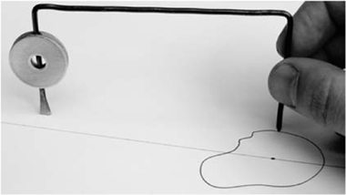
Figure 8.2. Using a hatchet planimeter.

What is the appropriate relation between the length of the planimeter and the maximum width of the shape whose area is to be measured? This is a practical question, and the general rule is that the maximum width of the shape should not exceed l, but this is a matter of compromise. The intrinsic mathematical error is reduced the greater the ratio l/ width is, but the penalty is that the proportional error in measuring the displacement is increased. If the width is too large, one option is to divide the shape into two or more parts and measure each separately. Conversely, if the shape is too small, trace around it twice before measuring the displacement.

The errors inherent in this planimeter will be discussed later. For now, it is interesting to start with a simple shape whose area is known. Try measuring the area of a square of diagonal width l or a circle of diameter l. The positions of the centres of mass are known, so start from there and then find out what happens if this starting point is deliberately misjudged. Record your results to get some feel for the accuracy of your planimeter and your own skill in using it.

It should be noted that the need to find the area of a plane shape is very common indeed, particularly in surveying and cartography. There are many other engineering applications where there is a need to calculate the area under a graph. For example, in calculating the work done by a steam engine a reading of pressure within the cylinder over time is drawn using what is known as an indicator, which we examined in section 3.2. The graph is drawn from a direct machine reading and the area under this graph needs to be measured accurately. For this to be practical it should be simple and quick.

The key to the operation of the hatchet planimeter is the observation that as the pointer traces around the curve, the knife blade follows in what is termed a pursuit curve. Recall that the tractrix of chapter 7 is an example of a pursuit curve. The blade does not slip sideways, but only moves forwards and backwards. This is why care is needed not to twist B and where some mass above A really helps. Actually, the theory behind this type of planimeter shows us that the measurements obtained give only an approximation to the area. Of course, there will be practical errors in any measurement, but those are different. There are planimeters that mathematically guarantee to measure the exact area and we shall describe two of these as well, together with the source of mathematical error in the hatchet planimeter.

8.1 What Is Area?

In order to understand how a planimeter works we really need to discuss what area actually is. In a similar way that length quantifies the extent of a one-dimensional line, area quantifies the space occupied by a two-dimensional plane shape. We usually only consider the lengths of straight lines, but many curves can in fact be measured by using a wheel to roll along the curve. The length of a straight line with the same total roll as the curve is said to be the length of the curve. This idea is used in a map measurer, which can be used with an appropriate scale to find the length of a proposed journey. Area is defined in terms of length using the following simple rules.

1. The area of a rectangle is the product of the lengths of the sides. So, the area of the rectangle in figure 8.3 is a × b
2. If we cut a shape into parts, the area of the original shape is the sum of the areas of the parts.

Figure 8.3. A plane rectangle.

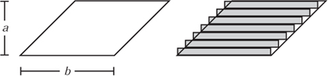
Figure 8.4. Dividing a parallelogram into small rectangles.

The first of these rules is the very basis of area and the second seems perfectly reasonable. However, with the second are you sure it does not matter how you decide to cut a shape up? It is a consequence of the second that the example in section 9.6 is impossible. Many of the properties that we expect from area are further consequences of these simple rules. For example, area is unaffected by rotation or translation in the plane. This means that we can move shapes around without changing their areas. The second rule holds even if one cuts a shape up into an infinite number of parts. For example, look back at figure 6.5. This shape is dissected into an infinite number of pieces and yet these sum to a finite area. The possibility for an infinite division gives area some very interesting and counter-intuitive properties.

Using these rules we will illustrate how to calculate the areas of various common shapes. Since area is based on rectangles, we shall start by using rectangles to calculate the areas of some simple and well-known shapes. The first of these is the parallelogram, which can be modelled very effectively with blocks or identically sized books.

Let us take a parallelogram, as shown in figure 8.4. We shall approximate this area by n thin rectangles of width b and height a/n. Immediately we notice that this approximation is not perfect. Small triangles stick out on one side and other small triangles are missing on the other. In this case these errors cancel out, although we certainly cannot take this for granted. What is important is that as n increases, which is to say as we take more and more strips, we get a better and better approximation to the parallelogram.

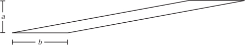
Figure 8.5. A stretched parallelogram.

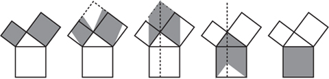
Figure 8.6. The Pythagorean theorem via parallelograms.

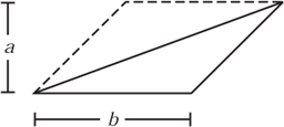
Figure 8.7. Area of a triangle via parallelograms.

This model is easy to assemble from n identical blocks. Once assembled, slide them horizontally until they are all one above each other. Since area is preserved by translation in the plane we immediately see that the area of the parallelogram is equal to the rectangle of width b and height a. This means that however far we slide the blocks, the area of a parallelogram remains constant. The parallelogram in figure 8.5 has the same area as those in figure 8.4. Manipulations of parallelograms can be used to provide another demonstration of the Pythagorean theorem, which is shown using the five pictures in figure 8.6. Notice the use of shears and translations to turn squares into parallelograms, move them, and then shear them back into a single square.

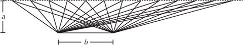
Figure 8.8. Moving the vertex of a triangle parallel to the base.

Figure 8.9. The Pythagorean theorem via triangles.

The next simplest shape is the triangle, such as that shown in figure 8.7. This can be seen as sitting inside a parallelogram which in fact contains two identical triangles. Therefore, the area of a triangle is half the product of the base b and the height a. That is ab. Again, we may move the apex of the triangle in a way that is parallel to the base without altering the area. All the triangles in figure 8.8 have identical area.

The previous demonstration of the Pythagorean theorem relied on shears and translations of parallelograms. The actual proof given by Euclid in book I, proposition 47 is different, and relies on shears and rotations of triangles. What he does is prove that half of the areas of each of the squares on the two sides combine to give half the area of the square on the hypotenuse. The argument given by Euclid relies on labelling the various points and justifying each step carefully using previously proved propositions. This proof amounts to the sequence of pictures in figure 8.9.

Another vitally important mathematical shape is the circle. Next we shall use shears, translations and rotations of triangles to show that the area of the circle of radius r is πr ². To do this, begin with a circle of radius r, which by the definition of π has circumference 2πr. This circle is divided up into n identical sectors (see figure 8.10). Next we cut up the circle into sectors and arrange these along a straight line as shown in figure 8.11. This does not affect the area. Now, the length of this line is, for large n at least, approximated very well by the circumference of the circle. Furthermore, the height of each sector is practically the radius of the circle. We shall approximate the area of each sector by such a triangle. You would be well advised to retain a suspicious attitude towards the cavalier way we forge ahead with approximations such as these. This notwithstanding, we can now move the apex of each triangle horizontally and gather these together in one place (see figure 8.12). Such a displacement of the apex does not alter the area. The area of this large triangle is clearly πr². Remember that this triangle is formed from the circle cut up into sectors, rearranged and with the individual triangles gathered together. Thus, we have the area of the circle also being πr².

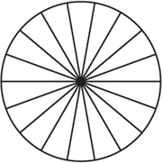
Figure 8.10. A circle divided into sectors.

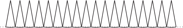
Figure 8.11. Sectors of a circle arranged on a line.

Figure 8.12. Gather the sectors to form a triangle.

It was Archimedes of Syracuse (287–212 B.C.E.) who first found this formula for the area of the circle and he gave it in his work Measurement of the Circle. He used a much more careful argument involving two sequences of regular polygons, one inside and one outside the circle. These sequences had an increasing number of sides and so approximate the circle with successively greater accuracy. In this way the circle is trapped between the inscribed and circumscribed polygons. It is possible to calculate the area of each polygon, so we also have two sequences of areas. These sequences both converge to the same quantity which must also be the area of the circle.

Many shapes can be decomposed into rectangles, triangles, circles and other regular shapes, and the areas of these shapes can therefore be calculated by summing the areas of their component parts. But what of an irregular shape, such as that shown in figure 8.2? How can we measure, or better still calculate, the area of such a shape? This problem appears to be much more difficult.

To illustrate why area is a difficult subject we give an example that begins to show how subtle the concept of area actually is. This shape, known as Koch’s snowflake curve, is constructed in stages, starting with an equilateral triangle with sides of length 1. Next construct a star of David shape, which is made by putting an equilateral triangle of side length onto each of the sides of the original triangle. This is shown in figure 8.13.

We extend this idea to construct a sequence of progressively more complicated shapes by putting an equilateral triangle onto the middle third of each of the sides. If this is continued indefinitely, the limiting shape is known as Koch’s snowflake. The first few stages in the construction are illustrated in figure 8.13.

The first shape has perimeter P₁ = 4. At every stage each side is replaced with four short sections, each one-third the length of the side they are replacing. Thus, if P_n is the perimeter of the nth stage, then

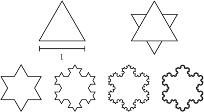
Figure 8.13. Koch’s snowflake curve.

An induction argument gives

This sequence increases indefinitely and becomes unbounded. So the limiting shape has an infinite perimeter.

As for the area, it is clear that this will fit into a large circle and hence is finite. However this is not good enough and we prefer to calculate it exactly. We noted in (1.1) that an equilateral triangle of side l has area . We started with l = 1, and at each stage we add 3.4^n-1 small equilateral triangles, each with sides of length 1/3ⁿ. The total area added gives the formula for the area A_n+11 as

Solving this, we have

Using (6.6) with r = we see that the total area of the limiting shape is

Thus, by constructing Koch’s snowflake we have produced a shape which encloses a finite area but which has an infinite perimeter! In fact such shapes appear to be excellent mathematical models for naturally occurring shapes such as coastlines, fractures and clouds.

Figure 8.14. Cantor’s set.

Area has some even stranger properties that the following example will help to reveal. We start with a solid filled-in square with sides of length 1. We shall remove vertical strips from this shape using the following scheme. We begin by removing a vertical strip of width . From the remaining two strips we remove two strips of width . This leaves four strips and from each of these we remove strips of width . This process is made to continue forever and at each stage we remove 2^n-1 strips of width . Hence, the total area removed at each stage is

If we continue this process indefinitely, it is clear that we will end up with a loose bundle of fibres. It is not clear that anything will remain; however, if two points with different x-coordinates are left, they will certainly end up on different fibres. The first seven stages of such a construction are shown in figure 8.14, in which the vertical height has been squashed severely for clarity.

In fact, the total area of material removed after n stages is only

which is another geometric progression. Using (6.6) again, this time with , we see that the total area removed is only

So the remaining bundle of fibres has an area of , even though it consists of an infinite collection of disjoint widthless vertical strips. Actually, we can repeat this process again and remove horizontal strips in exactly the same pattern. That is to say, beginning with a solid unit square, at each stage we shall remove 2^n-1 horizontal and vertical strips each of width . In doing this we shall remove at most a third of the remaining area leaving at least a third of the original area behind. However, this is now like a dust since any two distinct points remaining will be separated by previously removed vertical or horizontal strips or both. So a very fine and totally disconnected dust-like set of points can have a positive area!

8.2 Practical Measurement of Areas

Calculus is often encountered as a set of manipulations for doing such things as ‘differentiation’ and ‘integration’. Using integration to find the area under a graph is elegant, powerful and accurate. These techniques can be extended to other shapes in the plane where the boundary is described by a tidy mathematical equation. What about the data obtained when measuring the power output during the stroke of an engine cycle? This kind of experimental data certainly cannot be described exactly using perfect mathematical curves. Yet can we still measure the area under a graph such as this with mathematical accuracy?

The experiment at the beginning of the chapter claimed to relate an arbitrary plane area to a measurement obtained by tracing around the perimeter. Certainly this would be enough to measure the area under a graph: just trace around it. But what connection, if any, exists between area and perimeter? That a circle encloses the largest possible area for a fixed perimeter is a famous result known as the isoperimetric theorem. In the other direction, squashing a circle shows that a given perimeter may enclose a very small area. Next take a fixed area. Adapting the construction used for figure 8.13 demonstrates that there is no upper limit on the perimeter which can enclose this. Furthermore, a collection of separate widthless fibres, or a collection of specks of dust, can possess a significant positive area! Hence, there appears to be little or no connection between area and perimeter.

Given these subtleties, planimeters are extremely surprising. Note that we did not measure the perimeter in the experiment, we only traced around the boundary. This physical movement induced a displacement in the hatchet blade. So that these devices work we shall restrict ourselves to plane shapes: those that are a single connected piece, with no holes, and which have a smooth boundary, except at a finite number of corners. This removes the pathological examples such as those of figure 8.13 and similar monsters but, since a smooth boundary can wiggle an awful lot, we are still left with a particularly surprising, not to mention useful, result.

In fact, we shall discuss three different planimeters. The first is known as the linear planimeter, an example of which is shown in figure 8.19. The second kind is known as the polar planimeter or sometimes as the Amsler planimeter after its inventor. This was the most successful and common kind and many examples survive. Indeed, this type of planimeter may well still be in use. An example of such a planimeter is shown in figure 8.25, and an enlargement of part of it is shown in figure 8.26. The third planimeter is known as the hatchet planimeter or sometimes the Prytz planimeter, again after its inventor. After the complexity of the polar and linear planimeters it is disarmingly simple. However, the mathematics of the hatchet planimeter assures us only of an approximation to the area, whereas the mathematics of the polar and linear planimeters guarantees an exact result.

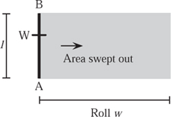
Figure 8.15. The area swept out by a line.

The basic operation of all planimeters is the same. To obtain a direct measurement of the area of a plane shape trace around the perimeter once in a clockwise direction. On the linear and polar planimeters the area is then read directly from a graduated counter that is part of the device. With the hatchet planimeter a separate ruler is needed. A comprehensive study of the types of planimeters available prior to 1894 can be found in Henrici (1894). The following geometrical explanations are based in part on this report.

8.3 Areas Swept Out by a Line

To start our discussion of the planimeter, consider a line AB of length l which moves a distance w to the right. As it moves, this line will sweep over a rectangle of area lw (see figure 8.15).

Suppose that a graduated wheel W is fixed using this line as an axle. As the line moves, the wheel will roll along. The total ‘roll’ of this wheel, given appropriate graduations and no slippage, will be the length w, just as with a map measurer. If the wheel is calibrated with l in mind, the area swept out may be read directly off this wheel.

In effect we have constructed a very simple planimeter, although since we can only measure areas of rectangles of length l this is practically useless. If the rod now moves vertically, no area will be swept out and the wheel will not roll. Again, the roll of the wheel gives the area swept out. Now consider the line moving diagonally across a parallelogram. The crucial observation is that the wheel will only record the component of the motion in the direction perpendicular to the line AB. As we showed above, the area of such a parallelogram is the product lw. Again, the roll as recorded on the wheel multiplied by the length gives us the area swept out by the line (see figure 8.16).

Figure 8.16. Moving the line across a parallelogram.

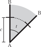
Figure 8.17. The rotating line.

Note that we have taken movement to the right to be positive roll. Similarly we take movement to the left to be negative roll and so consider the areas generated by a moving-line segment to be oriented. This means that we give area either a positive or a negative sign, and when adding such areas they can cancel each other out. Next consider the situation when we fix one end of the line at A and rotate the rod an angle t from B to B′ say (see figure 8.17). The roll recorded on the wheel will be the arc length w = ct. The area swept out by the rotating line will be

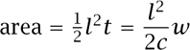
(as usual in mathematics we measure t in radians). Note that the area swept out is again proportional to the roll and also to the distance of the wheel from one end of the line.

In general, a line segment moving in the plane will sweep out an area and the direction of motion will dictate whether this area is considered positive or negative. Such a motion will contain both rotation and translation components. The fact that the three planimeters we discuss below work is justified by considering the areas swept out by moving-line segments. Of course, the justification above only applies to shapes with length l, so this is not much use. We shall remove this restriction in the next section.

Before we give an explanation of the mathematics behind the planimeter we comment on the wheel actually used on linear and polar planimeters. It is mounted on a short axle which is parallel to but slightly offset from AB. The wheel is connected by a worm gear to a counter and the wheel itself is read using a Vernier scale (discussed in section 4.5). The mechanism from an Allbrit 6000 planimeter is shown in figure 8.26. On this particular model the whole wheel mechanism can be moved along the line AB and positioned with the aid of another Vernier scale. This is to change a constant of proportionality, effectively changing l, so that when correctly set a direct reading of area can be taken in square centimetres, square inches or from a variety of scale diagrams. A detachable magnifying glass, not shown, is provided to help in accurate reading of the scales.

8.4 The Linear Planimeter

The linear planimeter incorporates the line AB, just as above, with a wheel at W. This time the point at A is constrained to run in a straight line, perhaps in a track or groove, such as that in the schematic of figure 8.18. Although this design was not as popular as the polar planimeter that we shall discuss in detail in section 8.5, commercial devices were based on this configuration (see, for example, Snow 1903). More popular commercially were designs that mounted a pivot for point A on a trolley, again constraining A to move in a straight line. This overcomes the difficulties with large maps and plans where a track, such as that shown in figure 8.18, gets in the way of B and so obscures part of the area to be measured. An example of such a trolley is shown in figure 8.19. Here the trolley moves in a straight line and the point A can be found at the end of the arm that is perpendicular to the axle. The point B can be seen as a small circle in the magnifying glass and the wheel is enclosed in the rectangular box, together with a counter.

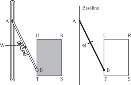
Figure 8.18. The linear planimeter.

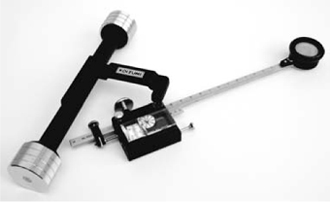
Figure 8.19. An example of a Koizumi linear roller planimeter.

To begin in a very simple way we shall measure the area of the arbitrary rectangle RSTU, shown in figure 8.18. We shall assume that the point B traces around the perimeter of this rectangle in a clockwise manner and that the point A is constrained to move in a line parallel to UT. Note that the dimensions of the rectangle are now arbitrary and the only restriction is that the length l, of the arm AB, must be sufficiently long to trace around the rectangle with A running in the track.

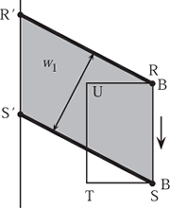
Figure 8.20. The motion of B from R to S.

During this motion, which is assumed to begin at R, B moves from R to S, then from S to T, and so on until B returns to R. We consider in detail the relationships between the roll as recorded on the wheel W and the area swept out by the line AB, and show that the total roll is proportional to the area exactly as before.

Consider first the motion of B along the edge from R to S. Since this is parallel to the track on which A is constrained, A will move in the same direction and it will move the same distance. During this motion the line AB sweeps out the shaded area shown in figure 8.20, and the wheel records a roll that is proportional to the normal component of the motion. That is to say, perpendicular to the line AB. This is the distance w₁ shown in figure 8.20. Since w₁ is the height of the parallelogram RSR′S′ and the base is the length AB, which is l, the area swept out by this motion is lw₁.

Next the point B moves from S to T and, during this motion, the point A moves vertically, as shown in figure 8.21(a). For now we denote the roll as w₂. Next, assume that B moves from T to U. Once again, the line AB is translated and sweeps out a parallelogram, just as during the motion of B from R to S. This time the roll w₃ will be in the opposite direction and will therefore be negative. The area swept out will be -lw₃. This is shown in figure 8.21(b).

Lastly, we move B from U back to the initial position R. This roll is denoted by w₄. Notice that the movement from U to R is exactly the opposite of the movement from S to T but translated vertically. Thus, by appealing to symmetry, we see that the roll w₂ must be equal to −w₄. Thus, the total recorded roll must be

Figure 8.21. The motions of B from S to T and from T to U.

w₁ + w₂ + w₃ + w₄ = w₁ + w₃.

If we multiply this reading by l, the length of AB, we have

lw₁ + lw₃ = lw₁ − (−lw₃) = area(RSR′S′) – area(TUT′U′).

Exactly as before we may slide the base of the parallelogram RSR′S′ along the baseline, along which A is constrained to move, without changing its area. If we transform both parallelograms RSR′S′ and TUT′U′ into rectangles, we can more easily see that the difference between these two areas is exactly the area of RSTU shown in figure 8.22. This shows that, by moving B round RSTU and multiplying the total roll recorded on W by the length of AB, we have the area of RSTU.

Of course, we have only succeeded in showing that our plan-imeter works for certain rectangles. Next we consider a compound shape consisting of two joined rectangles, as shown in figure 8.23. If we trace around the perimeters of RSTU as before and then round XTVW, we will be able to calculate the total area. Notice that in doing this we trace along the line TX twice, but in opposite directions. So the rolls recorded along this line cancel each other out. This leaves a total roll exactly the same as if we traced round the perimeter of the compound shape. Hence the total roll recorded by tracing the perimeter is exactly the roll recorded by tracing the two shapes separately.

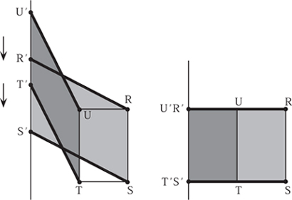
Figure 8.22. Translating the bases of the two parallelograms leaves their oriented areas unchanged.

Figure 8.23. Two adjacent rectangles.

Assume that a complicated shape can be cut up into adjoining rectangles. If we trace around each one separately, the roll along interior lines will cancel leaving us with the roll round the perimeter. Thus the area will be this reading multiplied by l. The only difficulty is when a shape with a smooth curved boundary, which cannot be dissected into a finite number of rectangles, needs to be considered: see, for example, figure 8.24. The usual approach is to say that ‘infinitely small’ rectangles make up the smooth shape, and so, strictly speaking, our argument breaks down here. However, in the case of a smooth boundary our planimeter still works. In fact we can cope with a finite number of kinks in the boundary but not a shape like the limiting form of the sequence generated by figure 8.13, which is decidedly unsmooth! In the case of a smooth, or finitely kinky, boundary the area will be found by reading the total roll and multiplying by the length l.

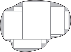
Figure 8.24. Tracing round a smooth boundary.

Figure 8.25. An example of a polar planimeter.

8.5 The Polar Planimeter of Amsler

The polar planimeter is very similar to the linear planimeter considered in the previous section. This design was first invented by Jacob Amsler (1823–1912) in the 1850s. This type of planimeter consists of two hinged arms, with the line AB as before, but this time A is fixed to another arm and so is constrained to move in a circle rather than a straight line. A schematic is shown in figure 8.27 and an actual planimeter in figure 8.25.

Figure 8.26. Details of the scales from an Allbrit 6000 planimeter.

Figure 8.27. The polar planimeter.

To use the instrument, place the pointer on the boundary of the shape, trace around the boundary of the shape in a clockwise direction and read off the total roll from the counter as before. We shall show in a moment that the total roll multiplied by the length of AB gives the area of the shape.

To justify why the polar planimeter works we shall use a similar geometrical argument. Let us consider the motion around the curved ‘rectangle’ RSTU shown in figure 8.28. This is again made up of four sections and just as before we consider the motion during each.

Figure 8.28. Tracing round a curved rectangle RSTU.

1. When moving from R to S the line AB slides and the roll recorded on the wheel will be w₁, the perpendicular component.
2. From S to T the line rotates about the angle t. We do not know what the roll recorded here will be but as before this will cancel out in a moment.
3. Next, from T to U we have a sliding motion and the roll recorded is the perpendicular distance w₂. This is in the opposite direction to w₁.
4. Finally, as the pointer moves from U to R we have the line rotating back in the opposite direction to its original position, i.e. through an angle of –t. During this motion the roll cancels out any roll during step 2 above.

Thus, just as before, the total roll recorded will be w₁ – w₂, and the area swept out will be this multiplied by the length of the line AB. The line passes over each point of the curvilinear parallelogram exactly once in the positive sense—any other points that it passes over it does so once forwards and once backwards. Hence the area of RSTU is the total roll multiplied by the length of AB. This argument, adapted from Cundy and Rollet (1961), is concluded by noticing that

[s]ince any area can be supposed divided into elementary curvilinear parallelograms of this type, the result is general.

This is analogous to dividing a shape into rectangles, as we did for the linear planimeter. Interestingly, our argument shows that the radius OA of the circle on which A is constrained to move does not enter into the equations which give us the area of the shape. Hence, we could (on very shaky ground indeed) connect the theory of the polar and linear planimeters by suggesting that a linear planimeter is nothing more than a polar planimeter in which the arm OA is infinitely long. Of course, this requires a huge leap of faith but does provide a conceptual link between the two, seemingly different, devices.

8.6 The Hatchet Planimeter of Prytz

So at last we come to the planimeter that was examined at the beginning of the chapter. This is known as the hatchet planimeter and was invented in 1875 by the Danish cavalry officer and mathematician Holgar Prytz, whose biography is given in Pedersen (1987). The device itself is disarmingly simple, really only consisting of a bent piece of metal, as shown in figure 8.2. As we shall see, the hatchet planimeter does not give the exact area but only an approximation. This is unlike the other planimeters detailed above, which are mathematically exact. Indeed, it is these errors that make this mathematically much more complex and interesting.

In practice if the distance l is sufficiently long compared with the width of the shape being measured and the starting line passes through the centre of mass of the shape, the mathematical error is very small indeed. Although the mathematical error may be reduced in this way, this improvement is more than cancelled out by the very much increased proportional error in the measurement of the displacement.

On the one hand we have mathematically exact but very complicated devices like the polar planimeter, and on the other a simple device that contains a small mathematical error. Superficially, the former would appear to be better, but since all physical devices contain some error in practice, which one results in the smallest overall practical error is far from obvious. For example, the linear and polar planimeters rely on the slip–roll interaction of the wheel. Many things can upset this. Friction in the wheel bearings, worm gears, etc., will certainly reduce the actual roll recorded. Corrosion on the wheel surface or the frictional qualities of the paper will introduce other, hard to quantify inaccuracies. Some planimeters solved this latter problem by providing a prepared surface on which the wheel rolls. The wheel and Vernier scale are marked out to allow readings to within 0.001 of a roll, and the whole carefully balanced roller spindle must be mounted exactly parallel to the line AB. Hence the simple hatchet planimeter, with a blade which can be easily sharpened at home, may well be a much more accurate solution. It is certainly the most economical, since Farthing (1985) quotes the starting cost of a polar planimeter as being £165 in 1982, which with inflation is equivalent to £400 in 2006.

The sources of the errors in the hatchet planimeter was a matter of much controversy, which was discussed in the journal Engineering during the period 1894–96. The discussion begins with a paper on ‘Integrating instruments’ by Henrici, which was read at the Physical Society on 23 March 1894. This was followed on 25 May 1894 by an article on p. 687 of Engineering giving a geometrical explanation of how the hatchet planimeter is able to measure a plane area. On 22 June 1894 Prytz gave a mathematical explanation of the source of error in the hatchet planimeter and on the same day various planimeters were discussed at another meeting of the Physical Society. This meeting is reported on pp. 26–27 of the 6 July issue of Engineering. There seems to have been some confusion as to the source of this error and in the 14 August 1896 issue of the journal (p. 205) Ernest Scott published some ‘improvements’. Actually, these amounted to little more than (i) being able to alter the length of the instrument and (ii) adding a wheel to record the final displacement by rolling the wheel back to its starting point, just like the recording wheel of the Amsler planimeter in fact. These modifications are illustrated in Scott’s figure 5 in his journal article. One of his other innovations was to replace the pointer with a rotating disc. Scott claims that in its original form the instrument, which he calls a stang planimeter, has ‘certain physical defects, which have probably been to a great extent the cause of the vague and erroneous statements one hears with regard to its theoretical accuracy’. He goes on to say that ‘the faults of the original stang planimeter were purely physical, and the writer ventures to think he has overcome these at a very slight extra expense by means of the above described improvements’. Actually, Scott was incorrect in asserting that the faults were physical: there are mathematical reasons why the hatchet planimeter only gives an approximation to the area.

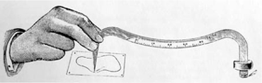
Figure 8.29. Goodman’s planimeter.

A week later, on 21 August 1896, there appears on pp. 255–56 an article titled ‘Goodman’s hatchet planimeter’. This claims to be another improvement on the hatchet planimeter that eliminates the sources of the errors. Goodman does eliminate one of the two sources of error in the hatchet planimeter by measuring arc length rather than linear displacement by means of a curved scale placed on the back of the instrument. This can be seen in figure 8.29. Of course, if the angle is small then the chord is an excellent approximation to the arc length. However, in this article he states that the starting point is chosen ‘somewhere near the centre of the figure; the exact position is, however immaterial’. This latter statement is incorrect since one source of error is only eliminated if the centre of mass is the initial point. Two letters appeared on p. 308 of Engineering on 4 September 1896 discussing the relative merits of Goodman’s and Scott’s ‘improvements’. However, a week later Prytz entered the fray with a reply. In this he criticizes Scott, saying that he ‘goes too far’ in his claim that the hatchet planimeter is ‘as accurate [as], if not more so than, the Amsler’. More importantly, he reasserts that the hatchet planimeter is not mathematically correct. He discusses the practical problems of using a very long hatchet planimeter to measure small areas and suggests that ‘this inconvenience may be removed by circumscribing the area two or more times before the end mark is set, as is indicated in the short explanation that accompanies every instrument’. For large areas he recommends dividing the area and measuring the parts. These two simple techniques completely remove the need for a changeable length planimeter. He also comments on the use of a wheel rather than the knife blade or keel.

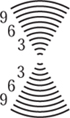
Figure 8.30. Prytz’s displacement scale.

I must remark that when the edge of the keel is grown dull, it is easy for any one to sharpen it a little. A wheel must ever be more sensible to dust and rough usage, and the more, the sharper and more accurately constructed it is.

Prytz goes on to complain further:

I wonder why Mr. Scott puts his name to the instrument instead of mine. He has on no point changed the principles for its use as a planimeter, and all the ‘improvements’ that he proposes are not new.

In an adjacent letter on p. 347 Prytz then rounds on Goodman, ending his letter with the following plea (see figure 8.30).

I must council the engineers, rather than use the ‘improved stang planimeters’ to let a country blacksmith make a copy of the original instrument, and, if they wish to avoid the measuring or calculating after a common rule, then, themselves to draw on the paper whereupon the keel glides a scale.

A week later on p. 337 of the 18 September edition of Engineering Goodman replies to both Scott and Prytz, ‘with the hope of easing their troubled minds’. His tone is far from conciliatory, and his letter closes as follows.

I have very good reasons for using the ‘bad form’ of the tracing points I do, and I think I know what I am about. I happen to have one of Captain Prytz’s planimeters, which I can quite believe may have been made by a country blacksmith; for my own part though, I prefer having mine made by a mathematical instrument maker, for curiously enough, I find the latter usually works more accurately that the former. Possibly in Denmark things are different.

Practical men have no time to waste in calculating the mean square of the radii of all the figures they require the area of. They want an instrument which gives a close approximation to the truth, without any calculation whatever. Such is mine. Let those who doubt get one and try for themselves.

So perhaps we should now explain why with the aid of the hatchet planimeter you are able to calculate a good approximation to the area of a plane shape. This will take a similar informal geometrical approach, using much that has been developed for the linear and polar planimeters. In doing this we shall point out the mathematical source of the discrepancy between what is measured by the hatchet planimeter and the true area of the shape being traced around. This will explain exactly what Prytz, Scott and Goodman were arguing about.

8.7 The Return of the Bent Coat-Hanger

To begin our discussion we shall return to our friend the line AB. In order to explain how the experiment at the beginning of the chapter is connected with the linear and polar planimeters we shall consider the line AB moving more generally in the plane.

To be more definite we assume that A and B each move once around a closed curve and return to their original positions. We assume further that during this motion the line does not make a complete revolution. We also assume that the situation is essentially that shown in figure 8.31, where B is always to the right of A. As before, we fix a wheel to the line using AB as an axle and at various points consider the roll recorded. To understand motion such as this we shall consider the moving line in two ways.

Figure 8.31. The area swept out by a line.

1. First we consider the microscopic, or rather infinitesimal, movement of the line and appeal to calculus.
2. Second we consider the macroscopic case, by application of pure geometry.

By relating these we will justify why the Prytz planimeter works. We sketch an informal argument that appeals to some simple ideas from calculus.

To begin, then, let us take a small motion, shown in figure 8.32, as the line moves from AB to A′B′. During any such very small motion the area swept out can be decomposed into two portions. The first is a rotating motion during which one end is fixed at A and the other moves from B to C. The second is a sliding motion from A to A′ when the other end moves from C to B′. We can approximate the total area swept out as the sum of the two components and, using previous calculations from section 8.3, we arrive at

infinitesimal area swept out	= area(ABCB′A′)
	= area(ACB′A′) + area(ABC)
	= ldw + l2 dt.

What we shall do is take infinitely small movements and sum these to calculate the area swept out during the whole motion shown in figure 8.31. By integrating such infinitesimally small dw and dt it is possible to show that the area swept out by the line AB is

Figure 8.32. A small motion of the line.

Moving A and B simultaneously around R_A and R_B, respectively, and returning them to their original positions, we have assumed that the line AB does not make a full revolution. Furthermore, the total angle sums to zero. Compare this argument—that the total angle is zero—with the symmetry of the rolls w₂ and w₄ in the argument for the linear planimeter. A consequence of no overall rotation is that the total roll recorded is due only to the sliding of the arm AB. Thus, the formula (8.1) reduces to

area swept out = l ∫ dw.

So, if w is the total recorded roll, then the total area swept out by the arm during the entire motion is lw, as before.

Turning to the macroscopic motion of the line we consider which areas of the plane are actually swept out during our motion. This is illustrated in figure 8.31, which you should compare with figure 8.22. The point B traces around the region R_B once. During this motion the line sweeps over the region once in a positive sense. Simultaneously, as the point A traces around R_A, the line sweeps over this region once in a negative sense. What about the region in between? It turns out that this is swept over as many times in the positive sense as in the negative sense so that, during the entire motion, the remaining area is exactly

This purely geometrical argument can be used in conjunction with the calculus argument to obtain the crucial relationship

Figure 8.33. A pursuit curve.

Notice that (8.3) is general for a line of fixed length in the plane when the end points move and return to their original positions and the whole line does not perform a complete revolution. Now we relate (8.3) to planimeters.

First we consider how the point A moves in a linear or polar planimeter. For the linear planimeter, A moves along a straight line, while for the polar planimeter, A moves forwards and backwards on an arc of a circle. In both cases the area of R_A, the region enclosed by the motion of A, is zero. Hence, (8.3) reduces to give area(R_B) equal to lw: the total recorded roll multiplied by the length of AB. What about the hatchet planimeter?

To help with the discussion, let us take the region R_B as shown in figure 8.33. The pointer begins its motion at the point B inside the region R_B as near as possible to the centre of mass of R_B. Begin the motion by moving along the straight line on which AB lies and then move around the boundary of the region R_B once in a clockwise direction. Finally, return along the line to the original position B. The key to the hatchet planimeter is the observation that as the pointer traces around the boundary of the region the knife blade follows in a pursuit curve. This curve of pursuit is a zigzag path arriving at A′ when the pointer returns to its original position. Imagine a wheel W fixed at the point A itself, using the line AB as an axle as before. Since the hatchet blade cannot move in a direction perpendicular to AB the total roll recorded along the pursuit curve from A to A′ will be zero.

Now, to use the formula (8.3) we must have a closed curve enclosing R_A. Therefore, to create a closed curve we imagine the hatchet blade being forced back to its original position A along a circular arc centred at B. This violates the non-slip condition. However, when we force the blade back to A, the roll recorded will be the arc length from A′ to A. Now if, as we have assumed, this angle is small, we can approximate the curve length AA′ well by the straight-line distance between A and A′.

We are now in a position to apply our formula (8.3), since A and B have completed their motion and returned to their original positions. Estimating the total ‘roll’ as the straight-line distance AA′ we have

area(R_B) − area(R_A) = area swept out ≈ lAA′.

Hence

area(R_B) ≈ lAA′ + area(R_A).

Now we see two sources of error:

1. the line AA′ approximates the circular arc AA′, with centre at B;
2. area(R_A) may not be zero.

To make sure that the first of these is small we take the length of AB to be long in relation to the maximum diameter of the shape we are trying to measure.

The area of R_A is a much more difficult problem. For the plan-imeter to work we must be able to ensure that this is very small. Draw a circle of radius l centred at the centre of mass of B. Part of R_A will be inside this and will have positive oriented area and part of R_A will lie outside this and will have negative area. Indeed, it can be shown that if the starting point of B is the centre of mass, then the area of R_A will be zero! However, finding the centre of mass is just as hard as calculating the area and so in practice one needs to make an educated guess and estimate the position.

The justification given here that each device works is not rigorous mathematics, rather it seeks to give an intuitive geometrical explanation. The polar planimeter can be justified rigorously using some advanced vector calculus and a result known as Green’s theorem—material that is often only encountered midway through a university mathematics degree. The details of this theory can be found in, for example, Gatterdam (1981). The error analysis of the hatchet planimeter is examined by Farthing (1985) and Crathorne (1908). That given by Foote (1998) employs even more advanced differential geometry.

8.8 Other Mathematical Integrators

Before the invention of the digital computer ingenious inventors devised mechanical instruments which performed a whole range of other calculations. These included finding the centre of mass, moment of inertia and so on. Some of these were based on the following disc integrator.

Imagine that we have a function f(x) that we wish to integrate. That is to say, we want to calculate f(x) dx. Imagine a horizontal disc which is spinning at a constant speed: one revolution per second, say. Riding on top of this is a vertical disc which is driven by the horizontal one. The axes of these two discs intersect and the distance of the vertical disc from the centre of the horizontal disc can be varied.

We build an input–output mechanism from this arrangement by taking the distance of the vertical disc from the centre of the horizontal disc as the input. We take t as a time variable and the output g(t) as the total rotation of the vertical disc. Now, the speed of rotation g′(t) will be proportional to the distance of the vertical disc from the centre of the horizontal disc. Since our input, f(t), is this distance, we have

g′(t) = kf (t),

where k is some constant of proportionality. Using the fundamental theorem of calculus we can solve the above equation to give g(t) as

g(t) = g(0) + k f(x) dx.

The device essentially integrates the input. Of course, there are many subtleties associated with such a device. Errors occur due to the very subtle slip–roll interaction and other physical problems—see Hele Shaw (1885) for more explanation. To do anything useful the force or movement needs to be amplified, perhaps with a configuration of linkages as in chapter 2. However, before the invention of the digital computer, such integrators were being chained together to solve complex differential equations. This is itself an application about which whole books have been written. You could construct models of such devices. In a straightforward survey article on this subject, Hartree (1938) comments as follows.

My first impression on seeing the photographs of Dr Bush’s machine was that they looked as if someone had been enjoying himself with an extra large Meccano set. This suggested the possibility of trying to build . . . a model version of the machine. . . . The result was successful beyond expectation; we found it possible to build almost entirely in Meccano, a model differential analyser, which would work not only qualitatively but quantitatively to an accuracy of about 2 per cent.

Indeed, Hartree mentions the construction of such devices as school projects.