A common cause of slow SQL Server performance is a heavy database application workload—the nature of the queries themselves. Thus, to analyze the cause of a system bottleneck, it is important to examine the database application workload and identify the SQL queries causing the most stress on system resources. To do this, you use the SQL Profiler and Management Studio tools.
In this chapter, I cover the following topics:
How to analyze SQL Server workload and identify costly SQL queries using SQL Profiler
How to combine the baseline measurements with data collected from SQL Profiler
How to analyze the processing strategy of a costly SQL query using Management Studio
How to track query performance through dynamic management views
How to analyze the effectiveness of index and join strategies for a SQL query
How to measure the cost of a SQL query using SQL utilities
SQL Profiler is a GUI and set of system stored procedures that can be used to do the following:
Graphically monitor SQL Server queries
Collect query information in the background
Analyze performance
Diagnose problems such as deadlocks
Debug a Transact-SQL (T-SQL) statement
Replay SQL Server activity in a simulation
You can also use SQL Profiler to capture activities performed on a SQL Server instance. Such a capture is called a Profiler trace. You can use a Profiler trace to capture events generated by various subsystems within SQL Server. You can run traces from the graphical front end or through direct calls to the procedures. The most efficient way to define a trace is through the system procedures, but a good place to start learning about traces is through the GUI.
Open the Profiler tool from the Start
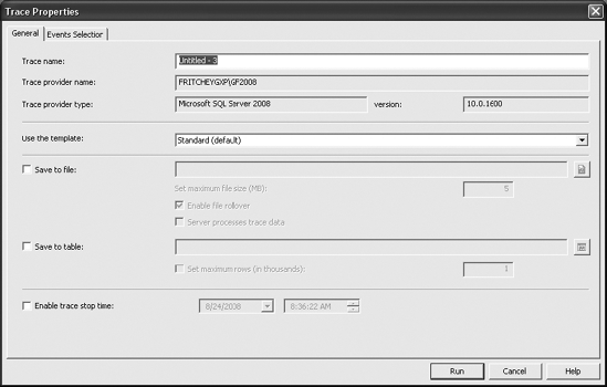
You can supply a trace name to help categorize your traces later when you have lots of them. Different trace templates are available that quickly help you set up new traces for different purposes. For the moment, I'll stick with the Standard trace. Without additional changes, this trace will run as a graphical trace, but from the Trace Properties dialog box you can define the trace to save its output to a file or to a table. I'll spend more time on these options later in this chapter. Finally, from the General tab, you can define a stop time for the trace. These options combine to give you more control over exactly what you intend to monitor and how you intend to monitor it within SQL Server.
With the initial setup complete, click the Events Selection tab to provide more detailed definition to your trace, as shown in Figure 3-2.
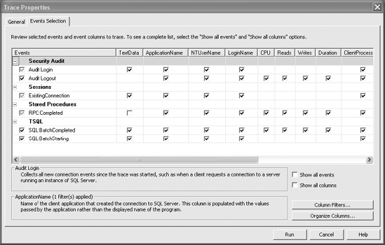
An event represents various activities performed in SQL Server. These are categorized for easy classification into event classes; cursor events, lock events, stored procedure events, and T-SQL events are a few common event classes.
For performance analysis, you are mainly interested in the events that help you judge levels of resource stress for various activities performed on SQL Server. By resource stress, I mean things such as the following:
What kind of CPU utilization was involved for the SQL activity?
How much memory was used?
How much I/O was involved?
How long did the SQL activity take to execute?
How frequently was a particular query executed?
What kind of errors and warnings were faced by the queries?
You can calculate the resource stress of a SQL activity after the completion of an event, so the main events you use for performance analysis are those that represent the completion of a SQL activity. Table 3-1 describes these events.
Table 3.1. Events to Trace Query Completion
Event Class | Event | Description |
|---|---|---|
|
| An RPC completion event |
| A stored procedure completion event | |
| A SQL statement completion event within a stored procedure | |
|
| A T-SQL batch completion event |
| A T-SQL statement completion event |
An RPC event indicates that the stored procedure was executed using the Remote Procedure Call (RPC) mechanism through an OLEDB command. If a database application executes a stored procedure using the T-SQL EXECUTE statement, then that stored procedure is resolved as a SQL batch rather than as an RPC. RPC requests are generally faster than EXECUTE requests, since they bypass much of the statement parsing and parameter processing in SQL Server.
A T-SQL batch is a set of SQL queries that are submitted together to SQL Server. A T-SQL batch is usually terminated by a GO command. The GO command is not a T-SQL statement. Instead, the GO command is recognized by the sqlcmd utility, as well as by Management Studio, and it signals the end of a batch. Each SQL query in the batch is considered a T-SQL statement. Thus, a T-SQL batch consists of one or more T-SQL statements. Statements or T-SQL statements are also the individual, discrete commands within a stored procedure. Capturing individual statements with the SP:StmtCompleted or SQL:StmtCompleted event can be a very expensive operation, depending on the number of individual statements within your queries. Assume for a moment that each stored procedure within your system contains one, and only one, T-SQL statement. In this case, the collection of completed statements is pretty low. Now assume that you have multiple statements within your procedures and that some of those procedures are calls to other procedures with other statements. Collecting all this extra data now becomes a noticeable load on the system. Statement completion events should be collected extremely judiciously, especially on a production system.
After you've selected a trace template, a preselected list of events will already be defined on the Events Selection tab. Only the events you have selected will be displayed. To see the full list of events available, click the Show All Events check box. To add an event to the trace, find the event under an event class in the Event column, and click the check box to the left of it. To remove events not required, deselect the check box next to the event.
Although the events listed in Table 3-1 represent the most common events used for determining performance, you can sometimes use a number of additional events to diagnose the same thing. For example, as mentioned in Chapter 1, repeated recompilation of a stored procedure adds processing overhead, which hurts the performance of the database request. The Stored Procedures event class of the Profiler tool includes an event, SP:Recompile, to indicate the recompilation of a stored procedure (this event is explained in depth in Chapter 10). Similarly, Profiler includes additional events to indicate other performance-related issues with a database workload. Table 3-2 shows a few of these events.
Table 3.2. Events to Trace Query Performance
Event Class | Event | Description |
|---|---|---|
|
| Keeps track of database connections when users connect to and disconnect from SQL Server. |
|
| Represents all the users connected to SQL Server before the trace was started. |
|
| Indicates that the cursor type created is different from the requested type. |
|
| Represents the intermediate termination of a request caused by actions such as query cancellation by a client or a broken database connection. |
| Indicates the occurrence of an exception in SQL Server. | |
| Indicates the occurrence of any warning during the execution of a query or a stored procedure. | |
| Indicates the occurrence of an error in a hashing operation. | |
| Indicates that the statistics of a column, required by the optimizer to decide a processing strategy, are missing. | |
| Indicates that a query is executed with no joining predicate between two tables. | |
| Indicates that a sort operation performed in a query such as | |
|
| Flags the presence of a deadlock. |
| Shows a trace of the chain of queries creating the deadlock. | |
| Signifies that the lock has exceeded the timeout parameter, which is set by | |
|
| Indicates that an execution plan for a stored procedure had to be recompiled, because one did not exist, a recompilation was forced, or the existing execution plan could not be reused. |
| Represents the starting of a stored | |
|
| Provides information about a database transaction, including information such as when a transaction started/completed, the duration of the transaction, and so on. |
Events are represented by different attributes called data columns. The data columns represent different attributes of an event, such as the class of the event, the SQL statement for the event, the resource cost of the event, and the source of the event.
The data columns that represent the resource cost of an event are CPU, Reads, Writes, and Duration. As a result, the data columns you will use most for performance analysis are shown in Table 3-3.
Table 3.3. Data Columns to Trace Query Completion
Data Column | Description |
|---|---|
| Type of event, for example, |
| SQL statement for an event, such as |
| CPU cost of an event in milliseconds (ms). For example, |
| Number of logical reads performed for an event. For example, |
| Number of logical writes performed for an event. |
| Execution time of an event in ms. |
| SQL Server process identifier used for the event. |
| Start time of an event. |
Each logical read and write consists of an 8KB page activity in memory, which may require zero or more physical I/O operations. To find the number of physical I/O operations on a disk subsystem, use the System Monitor tool; I'll cover more about combining the output of Profiler and System Monitor later in this chapter.
You can add a data column to a Profiler trace by simply clicking the check box for that column. If no check box is available for a given column, then the event in question cannot collect that piece of data. Like the events, initially only the data columns defined by the template are displayed. To see the complete list of data columns, click the Show All Columns check box.
You can use additional data columns from time to time to diagnose the cause of poor performance. For example, in the case of a stored procedure recompilation, the Profiler tool indicates the cause of the recompilation through the EventSubClass data column. (This data column is explained in depth in Chapter 10.) A few of the commonly used additional data columns are as follows:
BinaryDataIntegerDataEventSubClassDatabaseIDObjectIDIndexIDTransactionIDErrorEndTime
The BinaryData and IntegerData data columns provide specific information about a given SQL Server activity. For example, in the case of a cursor, they specify the type of cursor requested and the type of cursor created. Although the names of these additional data columns indicate their purpose to a great extent, I will explain the usefulness of these data columns in later chapters as you use them.
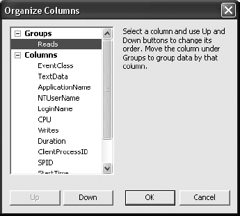
Column data can be rearranged to make the screen more pleasing, and they can be grouped to provide aggregates of the data collected. To control the column data placement, click the Organize Columns button. This opens the Organize Columns dialog box shown in Figure 3-3.
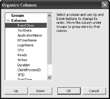
You can change the position of a column by clicking the Up and Down buttons. Moving a column into the Groups category means it will become an aggregation column.
In addition to defining events and data columns for a Profiler trace, you can also define various filter criteria. These help keep the trace output small, which is usually a good idea. Table 3-4 describes the filter criteria that you will commonly use during performance analysis.
Table 3.4. SQL Trace Filters
Events | Filter Criteria Example | Use |
|---|---|---|
|
| This filters out the events generated by Profiler. This is the default behavior. |
|
| This filters out events generated by a particular database. You can determine the ID of a database from its name as follows: |
|
| For performance analysis, you will often capture a trace for a large workload. In a large trace, there will be many event logs with a |
|
| This is similar to the criterion on the |
|
| This troubleshoots queries sent by a specific database user. |
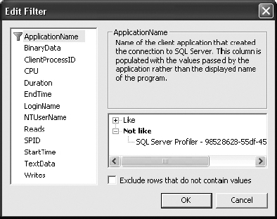
Figure 3-4 shows a snippet of the preceding filter criteria selection in SQL Profiler.
Note
For a complete list of filters available in SQL Profiler, please refer to the MSDN article "Limiting Traces" (http://msdn.microsoft.com/library/default.asp?url=/library/en-us/adminsql/ad_mon_perf_6nxd.asp).
In the previous section, you learned how to define a new Profiler trace to monitor activities using SQL Server. However, instead of defining a new trace every time you want to use one, you can create a trace template with your customized events, data columns, and filters and then reuse the trace template to capture a trace. The procedure for defining a new trace template is similar to that of defining a new trace:
Create a new trace.
Define the events, data columns, and filters the same way as shown earlier.
Save the trace definition as a trace template from the File

After you've defined a trace, clicking the Run button will begin capturing events and displaying them on your screen, as shown in Figure 3-5. You will see a series of events scrolling by, and you can watch your system perform in what I've always called SQL TV. You have control over the trace more or less like a DVD player, so you can pause, start, and stop the trace (sorry, no fast-forward) using the buttons on the toolbar. You can even pause the trace and make changes to it as you work.
Once you finish capturing your SQL Server activities, you can save the trace output to a trace file or a trace table. Trace output saved to a trace file is in a native format and can be opened by Profiler to analyze the SQL queries. Saving the trace output to a trace table allows the SQL queries in the trace output to be analyzed by Profiler as well as by SELECT statements on the trace table.
Profiler creates a trace table dynamically as per the definition of the data columns in the trace output. The ability to analyze the trace output using SELECT statements adds great flexibility to the analysis process. For example, if you want to find out the number of query executions with a response time of less than 500 ms, you can execute a SELECT statement on the trace table as follows:
SELECT COUNT(*) FROM <Trace Table>
WHERE Duration > 500
You will look at some sample queries in the "Identifying Costly Queries" section later in the chapter, but first I'll describe how to automate Profiler and simultaneously reduce the amount of memory and network bandwidth that the Profiler process uses.
The Profiler GUI makes collecting Profiler trace information easy. Unfortunately, that ease comes at a cost. The events captured by the Profiler tool go into a cache in memory in order to feed across the network to the GUI. Your GUI is dependent on your network. Network traffic can slow things down and cause the cache to fill. This will, to a small degree, impact performance on the server. Further, when the cache fills, the server will begin to drop events in order to avoid seriously impacting server performance. How do you avoid this? Use the system stored procedures to generate a scripted trace that outputs to a file.
You can create a scripted trace in one of two ways, manually or with the GUI. Until you get comfortable with all the requirements of the scripts, the easy way is to use the Profiler tool's GUI. These are the steps you'll need to perform:
Define a trace.
Click the menu File
You must select the target server type, in this instance, For SQL Server 2005/2008.
Give the file a name, and save it.
These steps will generate all the script commands that you need to capture a trace and output it to a file. You can also script trace events that will be used with the new 2008 Data Collector service, but that functionality is beyond the scope of this book.
To manually launch this new trace, use Management Studio as follows:
Open the file.
Replace where it says
InsertFileNameHerewith the appropriate name and path for your system.Execute the script. It will return a single column result set with the
TraceId.
You may want to automate the execution of this script through the SQL Agent, or you can even run the script from the command line using the sqlcmd.exe utility. Whatever method you use, the script will start the trace. If you have not defined a trace stop time, you will need to stop the trace manually using the TraceId. I'll show how to do that in the next section.
If you look at the scripts defined in the previous section, you will see a series of commands, called in a specific order:
sp_trace_create: Create a trace definition.sp_trace_setevent: Add events and event columns to the trace.sp_trace_setfilter: Apply filters to the trace.
Once the SQL trace has been defined, you can run the trace using the stored procedure sp_trace_setstatus.
The tracing of SQL activities continues until the trace is stopped. Since the SQL tracing continues as a back-end process, the Management Studio session need not be kept open. You can identify the running traces by using the SQL Server built-in function fn_trace_getinfo, as shown in the following query:
SELECT * FROM ::fn_trace_getinfo(default);
Figure 3-6 shows the output of the function.
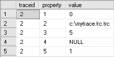
The number of unique traceids in the output of the function fn_trace_getinfo indicates the number of traces active on SQL Server. The data value of the column value for the property of 5 indicates whether the trace is running (value = 1) or stopped (value = 0). You can stop a specific trace, say traceid = 1, by executing the stored procedure sp_trace_setstatus:
EXEC sp_trace_setstatus 1, 0;
After a trace is stopped, its definition must be closed and deleted from the server by executing sp_trace_setstatus:
EXEC sp_trace_setstatus 1, 2;
To verify that the trace is stopped successfully, reexecute the function fn_trace_getinfo, and ensure that the output of the function doesn't contain the traceid.
The format of the trace file created by this technique is the same as that of the trace file created by Profiler. Therefore, this trace file can be analyzed in the same way as a trace file created by Profiler.
Capturing a SQL trace using stored procedures as outlined in the previous section avoids the overhead associated with the Profiler GUI. It also provides greater flexibility in managing the tracing schedule of a SQL trace than is provided by the Profiler tool. In Chapter 16, you will learn how to control the schedule of a SQL trace while capturing the activities of a SQL workload over an extended period of time.
Note
The time captured through a trace defined as illustrated in this section is stored in microseceonds, not milliseconds. This difference between units can cause confusion if not taken into account.
In Chapter 2, I showed how to capture Performance Monitor data to a file. In the preceding section, I showed how to capture Profiler data to a file as well. If you automate the collection of both of these sets of data so that they cover the same time periods, you can use them together inside the SQL Profiler GUI. Be sure that your trace has both the StartTime and Endtime data fields. Follow these steps:
Open the trace file.
Click the File
Select the Performance Monitor file to be imported.
Performing these actions will open the dialog box shown in Figure 3-7, which allows you to pick Performance Monitor counters for inclusion.
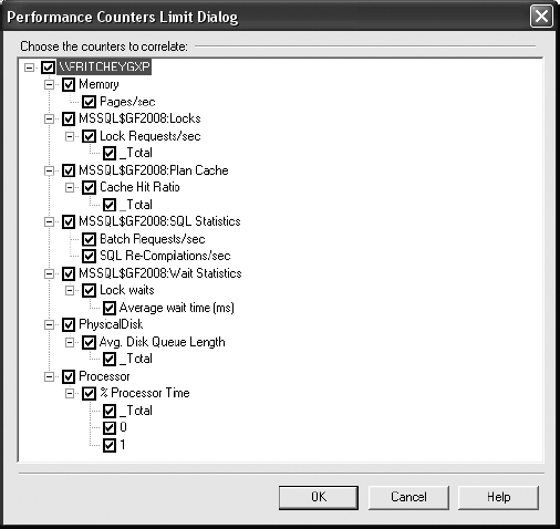
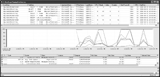
Once you've selected the counters you want to include, clicking OK will open the Profiler and Performance Monitor data together, as you can see in Figure 3-8. Now you can begin to use the trace data and the Performance Monitor data together. If you select an event in the top window, it will place a red line within the Performance Monitor data, showing where the event occurred within the time frame of that data. Conversely, you can click within the Performance Monitor data, and the event that represents that time frame will be selected. These capabilities work so well together that you'll be using them regularly during tuning sessions to identify the bottlenecks and stress points and to determine which specific queries are causing them.
You have already seen how to set some filters on a trace to help minimize the impact of Profiler on system resources. To further minimize the impact, consider the following suggestions:
Limit the number of events and data columns.
Discard start events for performance analysis.
Limit trace output size.
Avoid online data column sorting.
Run Profiler remotely.
In the following sections, I cover each of these suggestions in more depth.
While tracing SQL queries, you can decide which SQL activities should be captured by filtering events and data columns. Choosing extra events contributes to the bulk of tracing overhead. Data columns do not add much overhead, since they are only attributes of an event class. Therefore, it is extremely important to know why you want to trace each event selected and to select your events based only on necessity.
Minimizing the number of events to be captured prevents SQL Server from wasting the bandwidth of valuable resources generating all those events. Capturing events such as locks and execution plans should be done with caution, because these events make the trace output very large and degrade SQL Server's performance.
It's important to reduce the number of events while analyzing a production server, since you don't want the profiler to add a large amount of load to the production server. On a test server, the amount of load contributed by Profiler is a lesser consideration than the ability to analyze every activity on SQL Server. Therefore, on a test server, you need not compromise so much with the information you might be interested in.
Some events come with added cost. I mentioned earlier in the chapter that the statement completion events can be costly, but other events could negatively impact your system while you're attempting to capture information about that system.
The information you want for performance analysis revolves around the resource cost of a query. Start events, such as SP:StmtStarting, do not provide this information, because it is only after an event completes that you can compute the amount of I/O, the CPU load, and the duration of the query. Therefore, while tracking slow-running queries for performance analysis, you need not capture the start events. This information is provided by the corresponding completion events.
So, when should you capture start events? Well, you should capture start events when you don't expect some SQL queries to finish execution because of error conditions or when you find frequent Attention events. An Attention event usually indicates that the user cancelled the query midway or the query timeout expired, probably because the query was running for a long time.
Besides prefiltering events and data columns, other filtering criteria limit the trace output size. Again, limiting size may cause you to miss interesting events if you're looking at overall system behavior. But if you're focusing on costly queries, a filter helps. From the Edit Filter dialog box, accessed by clicking the Column Filters button on the Events Selection tab, consider the following settings:
Duration – Greater than or equal: 2: SQL queries with a
Durationequal to 0 or 1 ms cannot be further optimized.Reads – Greater than or equal: 2: SQL queries with number of logical reads equal to 0 or 1 ms cannot be further optimized.
During performance analysis, you usually sort a trace output on different data columns (such as Duration, CPU, and Reads) to identify queries with the largest corresponding figures. If you sort offline, you reduce the activities Profiler has to perform while interacting with SQL Server. This is how to sort a captured SQL trace output:
Capture the trace without any sorting (or grouping).
Save the trace output to a trace file.
Open the trace file and sort (or group) the trace file output on specific data columns as required.
It is usually not a good practice to run test tools directly on the production server. Profiler has a heavy user interface; therefore, it is better to run it on another machine. Similar to System Monitor, Profiler should not be run through a terminal service session, because a major part of the tool still runs on the server. When collecting a trace output directly to a file, save the file locally where Profiler is being run. This is still a more resource-intensive operation than running Profiler through the system stored procedures as a server-side trace. That remains the best option.
Some events are more costly than others. As I mentioned previously, depending on the nature of the queries being generated, the statement completion events can be very costly. Other events to use judiciously, especially on a system that's already experiencing stress, are the Showplan XML events Performance:Showplan XML, Performance:Showplan XML for Query Compile, and Performance:Showplan XML Statistics Profile. Although these events can be useful, keep them off the production machine.
Setting up a trace allows you to collect a lot of data for later use, but the collection can be somewhat expensive, and you have to wait on the results. If you need to immediately capture performance metrics about your system, especially as they pertain to query performance, then the dynamic management view sys.dm_exec_query_stats is what you need. If you still need a historical tracking of when queries were run and their individual costs, a trace is still the better tool. But if you just need to know, at this moment, the longest-running queries or the most physical reads, then you can get that information from sys.dm_exec_query_stats.
Since sys.dm_exec_query_stats is just a view, you can simply query against it and get information about the statistics of query plans on the server. Table 3-5 shows some of the data returned from the query.
Table 3.5. sys.dm_exec_query_stats Output
Column | Description |
|---|---|
| Pointer that refers to the execution plan |
| Time that the plan was created |
| Last time the plan was used by a query |
| Number of times the plan has been used |
| Total CPU time used by the plan since it was created |
| Total number of reads used since the plan was created |
| Total number of writes used since the plan was created |
| A binary hash that can be used to identify queries with similar logic |
| A binary hash that can be used to identify plans with similar logic |
Table 3-5 is just a sampling. For complete details, see Books Online.
To filter the information returned from sys.dm_exec_query_stats, you'll need to join it with other dynamic management functions such as sys.dm_exec_sql_text, which shows the query text associated with the plan, or sys.dm_query_plan, which has the execution plan for the query. Once joined to these other DMFs, you can limit the database or procedure that you want to filter. These other DMFs are covered in detail in other chapters of the book.
Now that you have seen what you need to consider when using the Profiler tool, let's look at what the data represents: the costly queries themselves. When the performance of SQL Server goes bad, two things are most likely happening:
First, certain queries create high stress on system resources. These queries affect the performance of the overall system, because the server becomes incapable of serving other SQL queries fast enough.
Additionally, the costly queries block all other queries requesting the same database resources, further degrading the performance of those queries. Optimizing the costly queries improves not only their own performance but also the performance of other queries by reducing database blocking and pressure on SQL Server resources.
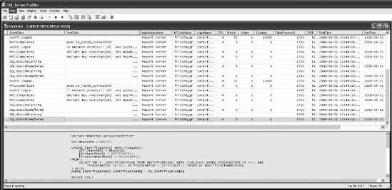
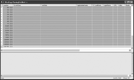
You can use Profiler to capture the SQL Server workload, as explained previously in this chapter. Define a trace. Then run the queries in trace_queries.sql. Figure 3-9 shows a sample trace output. On a live production server, the trace output may be quite large; the solution is to use filter criteria, as explained in the earlier "Filters" section, to limit the size of the trace output.
Once you have captured the set of SQL queries representing a complete workload, you should analyze the trace to identify two sets of queries:
Costly queries that are causing a great deal of pressure on the system resources
Queries that are slowed down the most
The goal of SQL Server is to return result sets to the user in the shortest time. To do this, SQL Server has a built-in, cost-based optimizer called the query optimizer, which generates a cost-effective strategy called a query execution plan. The query optimizer weighs many factors, including (but not limited to) the usage of CPU, memory, and disk I/O required to execute a query, all derived from the statistics maintained by indexes or generated on the fly, and it then creates a cost-effective execution plan. Although minimizing the number of I/Os is not a requirement for a cost-effective plan, you will often find that the least costly plan has the fewest I/Os because I/O operations are expensive.
In the data returned from a trace, the CPU and Reads columns also show where a query costs you. The CPU column represents the CPU time used to execute the query. The Reads column represents the number of logical pages (8KB in size) a query operated on and thereby indicates the amount of memory stress caused by the query. It also provides an indication of disk stress, since memory pages have to be backed up in the case of action queries, populated during first-time data access, and displaced to disk during memory bottlenecks. The higher the number of logical reads for a query, the higher the possible stress on the disk could be. An excessive number of logical pages also increases load on the CPU in managing those pages.
The queries that cause a large number of logical reads usually acquire locks on a correspondingly large set of data. Even reading (as opposed to writing) requires share locks on all the data. These queries block all other queries requesting this data (or a part of the data) for the purposes of modifying it, not for reading it. Since these queries are inherently costly and require a long time to execute, they block other queries for an extended period of time. The blocked queries then cause blocks on further queries, introducing a chain of blocking in the database. (Chapter 12 covers lock modes.)
As a result, it makes sense to identify the costly queries and optimize them first, thereby doing the following:
Improving the performance of the costly queries themselves
Reducing the overall stress on system resources
Reducing database blocking
The costly queries can be categorized into the following two types:
Single execution: An individual execution of the query is costly.
Multiple executions: A query itself may not be costly, but the repeated execution of the query causes pressure on the system resources.
You can identify these two types of costly queries using different approaches, as explained in the following sections.
Costly Queries with a Single Execution
You can identify the costly queries by analyzing a SQL Profiler trace output file or by querying sys.dm_exec_query_stats. Since you are interested in identifying queries that perform a large number of logical reads, you should sort the trace output on the Reads data column. You can access the trace information by following these steps:
Capture a Profiler trace that represents a typical workload.
Save the trace output to a trace file.
Open the trace file for analysis.
Open the Properties window for the trace, and click the Events Selection tab.
Open the Organize Columns window by clicking that button.
Group the trace output on the
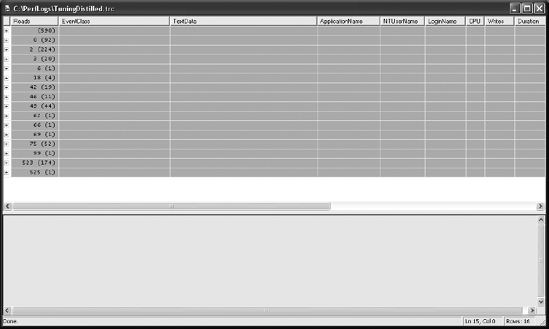
Readscolumn. To do this, move theReadscolumn under the Groups section, described earlier in this chapter, as shown in Figure 3-10.You can work with the trace grouped, or you can look at it sorted by changing the display using Ctrl+E.
This process will group the trace output on the Reads column, as shown in Figure 3-11. The trace output is sorted on Reads in ascending order. From there, you can select a few of the costliest queries and analyze and optimize them appropriately.
In some cases, you may have identified a large stress on the CPU from the System Monitor output. The pressure on the CPU may be because of a large number of CPU-intensive operations, such as stored procedure recompilations, aggregate functions, data sorting, hash joins, and so on. In such cases, you should sort the Profiler trace output on the CPU column to identify the queries taking up a large number of processor cycles.
Costly Queries with Multiple Executions
As I mentioned earlier, sometimes a query may not be costly by itself, but the cumulative effect of multiple executions of the same query might put pressure on the system resources. Sorting on the Reads column won't help you identify this type of costly query. You instead want to know the total number of reads performed by multiple executions of the query. Unfortunately, Profiler doesn't help here directly, but you can still get this information in the following ways:
Group the trace output in Profiler on the following columns:
EventClass,TextData, andReads. For the group of rows with the sameEventClassandTextData, manually calculate the total of all the correspondingReads. This approach doesn't sound very user friendly!Save the trace output to a trace table by selecting File
Access the
sys.dm_exec_query_statsDMV to retrieve the information from the production server. This assumes that you're dealing with an immediate issue and not looking at a historical problem.
In this case, I'll load the data into a table on the database so that I can run queries against it using the following script:
SELECT * INTO Trace_Table
FROM ::fn_trace_gettable('C:PerformanceTrace.trc', default)
Once the SQL trace is imported into a database table, execute a SELECT statement to find the total number of reads performed by the multiple executions of the same query as follows (reads.sql in the download):
SELECT COUNT(*) AS TotalExecutions, EventClass, TextData
  , SUM(Duration) AS Duration_Total
  , SUM(CPU) AS CPU_Total
  , SUM(Reads) AS Reads_Total
  , SUM(Writes) AS Writes_Total
FROM Trace_Table
GROUP BY EventClass, TextData
ORDER BY Reads_Total DESC
The TotalExecutions column in the preceding script indicates the number of times a query was executed. The Reads_Total column indicates the total number of reads performed by the multiple executions of the query.
However, there is a little problem. The data type of the TextData column for the trace table created by Profiler is NTEXT, which can't be specified in the GROUP BY clause—SQL Server 2008 doesn't support grouping on a column with the NTEXT data type. Therefore, you may create a table similar to the trace table, with the only exception being that the data type of the TextData column should be NVARCHAR(MAX) instead of NTEXT. Using the MAX length for the NVARCHAR data type allows you not to worry about how long the NTEXT data is.
Another approach is to use the CAST function as follows:
SELECT COUNT(*) AS TotalExecutions, EventClass
  , CAST(TextData AS NVARCHAR(MAX)) TextData
  , SUM(Duration) AS Duration_Total
  , SUM(CPU) AS CPU_Total
  , SUM(Reads) AS Reads_Total
  , SUM(Writes) AS Writes_Total
FROM Trace_Table
GROUP BY EventClass, CAST(TextData AS NVARCHAR(MAX))
ORDER BY Reads_Total DESC
The costly queries identified by this approach are a better indication of load than the costly queries with single execution identified by Profiler. For example, a query that requires 50 reads might be executed 1,000 times. The query itself may be considered cheap enough, but the total number of reads performed by the query turns out to be 50,000 (= 50 × 1,000), which cannot be considered cheap. Optimizing this query to reduce the reads by even 10 for individual execution reduces the total number of reads by 10,000 (= 10 × 1,000), which can be more beneficial than optimizing a single query with 5,000 reads.
The problem with this approach is that most queries will have a varying set of criteria in the WHERE clause or that procedure calls will have different values and numbers of parameters passed in. That makes the simple grouping by TextData impossible. You can take care of this problem with a number of approaches. One of the better ones is outlined on the Microsoft Developers Network at http://msdn.microsoft.com/en-us/library/aa175800(SQL.80).aspx. Although it was written originally for SQL Server 2000, it will work fine with SQL Server 2008.
Getting the same information out of the sys.dm_exec_query_stats view simply requires a query against the DMV:
SELECT  ss.sum_execution_count
       ,t.TEXT
       ,ss.sum_total_elapsed_time
       ,ss.sum_total_worker_time
       ,ss.sum_total_logical_reads
       ,ss.sum_total_logical_writes
FROM  (SELECT s.plan_handle
              ,SUM(s.execution_count) sum_execution_count
              ,SUM(s.total_elapsed_time) sum_total_elapsed_time
              ,SUM(s.total_worker_time) sum_total_worker_time
              ,SUM(s.total_logical_reads) sum_total_logical_reads
              ,SUM(s.total_logical_writes) sum_total_logical_writes
          FROM sys.dm_exec_query_stats s
          GROUP BY s.plan_handle
          ) AS ss
          CROSS APPLY sys.dm_exec_sql_text(ss.plan_handle) t
ORDER BY sum_total_logical_reads DESC
This is so much easier than all the work required to gather trace data that it makes you wonder why you would ever use trace data. The main reason is precision. The sys.dm_exec_query_stats view is a running aggregate for the time that a given plan has been in memory. A trace, on the other hand, is a historical track for whatever time frame you ran it in. You can even add traces together within a database and have a list of data that you can generate totals in a more precise manner rather than simply relying on a given moment in time. But understand that a lot of troubleshooting of performance problems is focused on that moment in time when the query is running slowly. That's when sys.dm_exec_query_stats becomes irreplaceably useful.
Because a user's experience is highly influenced by the response time of their requests, you should regularly monitor the execution time of incoming SQL queries and find out the response time of slow-running queries. If the response time (or duration) of slow-running queries becomes unacceptable, then you should analyze the cause of performance degradation. Not every slow-performing query is caused by resource issues, though. Other concerns such as blocking can also lead to slow query performance. Blocking is covered in detail in Chapter 12.
To discover the slow-running SQL queries, group a trace output on the Duration column. This will sort the trace output, as shown in Figure 3-12.
For a slow-running system, you should note the duration of slow-running queries before and after the optimization process. After you apply optimization techniques, you should then work out the overall effect on the system. It is possible that your optimization steps may have adversely affected other queries, making them slower.
Once you have identified a costly query, you need to find out why it is so costly. You can identify the costly query from SQL Profiler or sys.dm_exec_query_stats, rerun it in Management Studio, and look at the execution plan used by the query optimizer. An execution plan shows the processing strategy (including multiple intermediate steps) used by the query optimizer to execute a query.
To create an execution plan, the query optimizer evaluates various permutations of indexes and join strategies. Because of the possibility of a large number of potential plans, this optimization process may take a long time to generate the most cost-effective execution plan. To prevent the overoptimization of an execution plan, the optimization process is broken into multiple phases. Each phase is a set of transformation rules that evaluate various permutations of indexes and join strategies.
After going through a phase, the query optimizer examines the estimated cost of the resulting plan. If the query optimizer determines that the plan is cheap enough, it will use the plan without going through the remaining optimization phases. However, if the plan is not cheap enough, the optimizer will go through the next optimization phase. I will cover execution plan generation in more depth in Chapter 9.
SQL Server displays a query execution plan in various forms and from two different types. The most commonly used forms in SQL Server 2008 are the graphical execution plan and the XML execution plan. Actually, the graphical execution plan is simply an XML execution plan parsed for the screen. The two types of execution plan are the estimated plan and the actual plan. The estimated plan includes the results coming from the query optimizer, and the actual plan is the plan used by the query engine. The beauty of the estimated plan is that it doesn't require the query to be executed. These plan types can differ, but most of the time they will be the same. The graphical execution plan uses icons to represent the processing strategy of a query. To obtain a graphical estimated execution plan, select Query
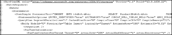
You can obtain the estimated XML execution plan for the costliest query identified previously using the SET SHOWPLAN_XML command as follows (set_showplan.sql in the download):
SET SHOWPLAN_XML ON
GO
SELECT  soh.AccountNumber,
        sod.LineTotal,
        sod.OrderQty,
        sod.UnitPrice,
        p.Name
FROM    Sales.SalesOrderHeader soh
        JOIN Sales.SalesOrderDetail sod
        ON soh.SalesOrderID = sod.SalesOrderID
        JOIN Production.Product p
        ON sod.ProductID = p.ProductID
WHERE sod.LineTotal > 1000 ; GO SET SHOWPLAN_XML OFF GO
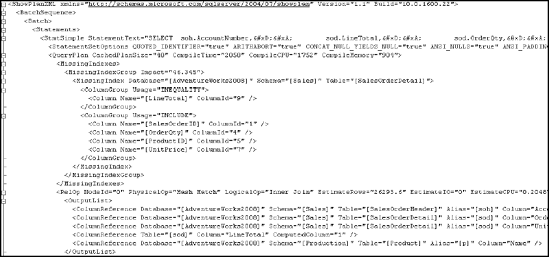
Running this query results in a link to an execution plan, not an execution plan or any data. Clicking the link will open an execution plan. Although the plan will be displayed as a graphical plan, right-clicking the plan and selecting Show Execution Plan XML will display the XML data. Figure 3-13 shows a portion of the XML execution plan output.
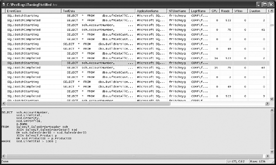
Let's start with the costly query identified in set_showplan.sql. Copy it (minus the SET SHOWPLAN_XML statements) into Management Studio, and turn on Include Actual Execution Plan. Now, on executing this query, you'll see the execution plan in Figure 3-14.
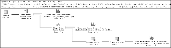
Read the execution plan from right to left and from top to bottom. Each step represents an operation performed to get the final output of the query. Some of the aspects of a query execution represented by an execution plan are as follows:
If a query consists of a batch of multiple queries, the execution plan for each query will be displayed in the order of execution. Each execution plan in the batch will have a relative estimated cost, with the total cost of the whole batch being 100 percent.
Every icon in an execution plan represents an operator. They will each have a relative estimated cost, with the total cost of all the nodes in an execution plan being 100 percent.
Usually a starting operator in an execution represents a data-retrieval mechanism from a database object (a table or an index). For example, in the execution plan in Figure 3-14, the three starting points represent retrievals from the
SalesOrderHeader,SalesOrderDetail, andProducttables.Data retrieval will usually be either a table operation or an index operation. For example, in the execution plan in Figure 3-11, all three data retrieval steps are index operations.
Data retrieval on an index will be either an index scan or an index seek. For example, the first and third index operations in Figure 3-14 are index scans, and the second one is an index seek.
The naming convention for a data-retrieval operation on an index is
[Table Name].[Index Name].Data flows from right to left between two operators and is indicated by a connecting arrow between the two operators.
The thickness of a connecting arrow between operators represents a graphical representation of the number of rows transferred.
The joining mechanism between two operators in the same column will be either a nested loop join, a hash match join, or a merge join. For example, in the execution plan shown in Figure 3-14, there is one nested loop join and one hash match.
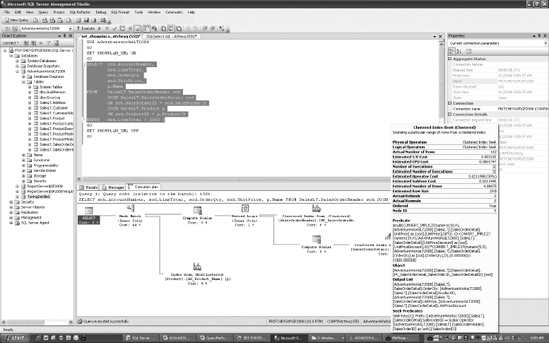
Running the mouse over a node in an execution plan shows a pop-up window with some details, as you can see in Figure 3-15.
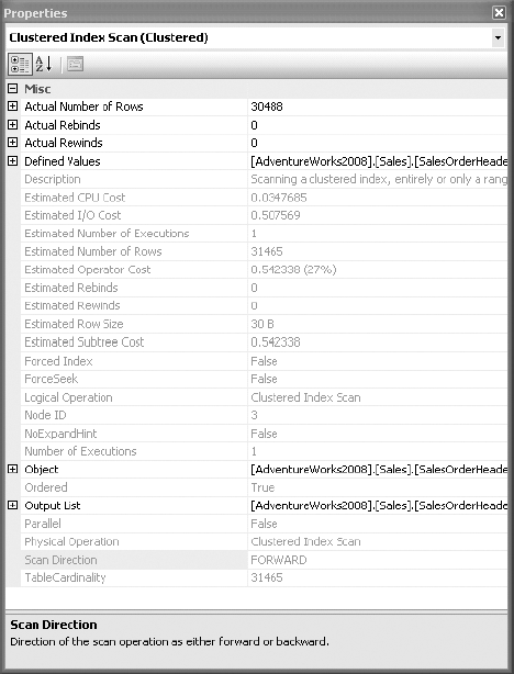
A complete set of details about an operator is available in the Properties window, which you can open by right-clicking the operator and selecting Properties. This is visible in Figure 3-16.
An operator detail shows both physical and logical operation types at the top. Physical operations represent those actually used by the storage engine, while the logical operations are the constructs used by the optimizer to build the estimated execution plan. If logical and physical operations are the same, then only the physical operation is shown. It also displays other useful information, such as row count, I/O cost, CPU cost, and so on.
The Argument section in an operator detail pop-up window is especially useful in analysis, because it shows the filter or join criterion used by the optimizer.
Your main interest in the execution plan is to find out which steps are relatively costly. These steps are the starting point for your query optimization. You can choose the starting steps by adopting the following techniques:
Each node in an execution plan shows its relative cost in the complete execution plan, with the total cost of the whole plan being 100 percent. Therefore, focus attention on the node(s) with the highest relative cost. For example, the execution plan in Figure 3-14 has two steps with 34 percent cost each.
An execution plan may be from a batch of statements, so you may also need to find the most costly statement. In Figure 3-15 and Figure 3-14, you can see at the top of the plan the text "Query 1." In a batch situation, there will be multiple plans, and they will be numbered in the order they occurred within the batch.
Observe the thickness of the connecting arrows between nodes. A very thick connecting arrow indicates a large number of rows being transferred between the corresponding nodes. Analyze the node to the left of the arrow to understand why it requires so many rows. Check the properties of the arrows too. You may see that the estimated rows and the actual rows are different. This can be caused by out-of-date statistics, among other things.
Look for hash join operations. For small result sets, a nested loop join is usually the preferred join technique. You will learn more about hash joins compared to nested loop joins later in this chapter.
Look for bookmark lookup operations. A bookmark operation for a large result set can cause a large number of logical reads. I will cover bookmark lookups in more detail in Chapter 6.
There may be warnings, indicated by an exclamation point on one of the operators, which are areas of immediate concern. These can be caused by a variety of issues, including a join without join criteria or an index or a table with missing statistics. Usually resolving the warning situation will help performance.
Look for steps performing a sort operation. This indicates that the data was not retrieved in the correct sort order.
To examine a costly step in an execution plan further, you should analyze the data-retrieval mechanism for the relevant table or index. First, you should check whether an index operation is a seek or a scan. Usually, for best performance, you should retrieve as few rows as possible from a table, and an index seek is usually the most efficient way of accessing a small number of rows. A scan operation usually indicates that a larger number of rows have been accessed. Therefore, it is generally preferable to seek rather than scan.
Next, you want to ensure that the indexing mechanism is properly set up. The query optimizer evaluates the available indexes to discover which index will retrieve data from the table in the most efficient way. If a desired index is not available, the optimizer uses the next best index. For best performance, you should always ensure that the best index is used in a data-retrieval operation. You can judge the index effectiveness (whether the best index is used or not) by analyzing the Argument section of a node detail for the following:
A data-retrieval operation
A join operation
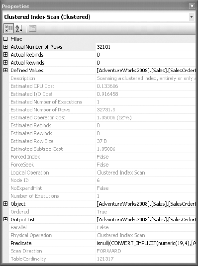
Let's look at the data-retrieval mechanism for the Product table in the previous execution plan (Figure 3-14). Figure 3-17 shows the operator properties.
In the operator properties for the SalesOrderDetail table, the Object property specifies the index used, PK_SalesOrderDetail. It uses the following naming convention: [Database].[Owner].[Table Name].[Index Name]. The Seek Predicates property specifies the column, or columns, used to seek into the index. The SalesOrderDetail table is joined with the SalesOrderHeader table on the SalesOrderId column. The SEEK works on the fact that the join criteria, SalesOrderId, is the leading edge of the clustered index and primary key, PK_SalesOrderDetail.
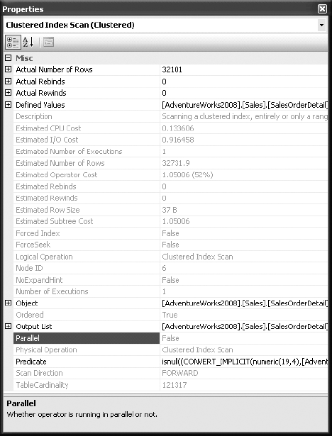
Sometimes you may have a different data-retrieval mechanism, as shown in Figure 3-18.
In the properties in Figure 3-18, there is no predicate. The lack of predicate means that the entire table, remembering that a clustered index is the table, is being scanned as input to the merge join operator (refer to the earlier Figure 3-14).
In addition to analyzing the indexes used, you should examine the effectiveness of join strategies decided by the optimizer. SQL Server uses three types of joins:
Hash joins
Merge joins
Nested loop joins
In many simple queries affecting a small set of rows, nested loop joins are far superior to both hash and merge joins. The join types to be used in a query are decided dynamically by the optimizer.
Hash Join
To understand SQL Server's hash join strategy, consider the following simple query (hash.sql in the download):
SELECT  p.*
FROM    Production.Product p
        JOIN Production.ProductSubCategory spc
        ON p.ProductSubCategoryID = spc.ProductSubCategoryID
Table 3-6 shows the two tables' indexes and number of rows.
Table 3.6. Indexes and Number of Rows of the Products and ProductCategory Tables
Table | Indexes | Number of Rows |
|---|---|---|
| Clustered index on | 295 |
| Clustered index on | 41 |
Figure 3-19 shows the execution plan for the preceding query.
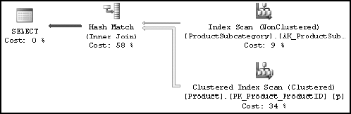
You can see that the optimizer used a hash join between the two tables.
A hash join uses the two join inputs as a build input and a probe input. The build input is shown as the top input in the execution plan, and the probe input is shown as the bottom input. The smaller of the two inputs serves as the build input.
The hash join performs its operation in two phases: the build phase and the probe phase. In the most commonly used form of hash join, the in-memory hash join, the entire build input is scanned or computed, and then a hash table is built in memory. Each row is inserted into a hash bucket depending on the hash value computed for the hash key (the set of columns in the equality predicate).
This build phase is followed by the probe phase. The entire probe input is scanned or computed one row at a time, and for each probe row, a hash key value is computed. The corresponding hash bucket is scanned for the hash key value from the probe input, and the matches are produced. Figure 3-20 illustrates the process of an in-memory hash join.
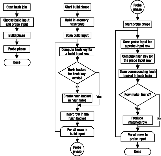
The query optimizer uses hash joins to process large, unsorted, nonindexed inputs efficiently. Let's now look at the next type of join: the merge join.
Merge Join
In the previous case, input from the Product table is larger, and the table is not indexed on the joining column (ProductCategoryID). Using the following simple query (merge.sql in the download), you can see different behavior:
SELECT  pm.*
FROM    Production.ProductModel pm
        JOIN Production.ProductModelProductDescriptionCulture pmpd
        ON pm.ProductModelID = pmpd.ProductModelID
Figure 3-21 shows the resultant execution plan for this query.
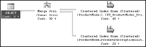
For this query, the optimizer used a merge join between the two tables. A merge join requires both join inputs to be sorted on the merge columns, as defined by the join criterion. If indexes are available on both joining columns, then the join inputs are sorted by the index. Since each join input is sorted, the merge join gets a row from each input and compares them for equality. A matching row is produced if they are equal. This process is repeated until all rows are processed.
In this case, the query optimizer found that the join inputs were both sorted (or indexed) on their joining columns. As a result, the merge join was chosen as a faster join strategy than the hash join.
Nested Loop Join
The final type of join I'll cover here is the nested loop join. For better performance, you should always access a limited number of rows from individual tables. To understand the effect of using a smaller result set, decrease the join inputs in your query as follows (loop.sql in the download):
SELECT  soh.*
FROM    Sales.SalesOrderHeader soh
        JOIN Sales.SalesOrderDetail sod
        ON soh.SalesOrderID = sod.SalesOrderID
WHERE   soh.SalesOrderID = 71832
Figure 3-22 shows the resultant execution plan of the new query.
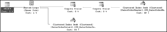
As you can see, the optimizer used a nested loop join between the two tables.
A nested loop join uses one join input as the outer input table and the other as the inner input table. The outer input table is shown as the top input in the execution plan, and the inner input table is shown as the bottom input table. The outer loop consumes the outer input table row by row. The inner loop, executed for each outer row, searches for matching rows in the inner input table.
Nested loop joins are highly effective if the outer input is quite small and the inner input is large but indexed. In many simple queries affecting a small set of rows, nested loop joins are far superior to both hash and merge joins. Joins operate by gaining speed through other sacrifices. A loop join is fast because it uses memory to take a small set of data and compare it quickly to a second set of data. A merge join similarly uses memory and a bit of tempdb to do its ordered comparisons. A hash join uses memory and tempdb to build out the hash tables for the join. Although a loop join is faster, it will consume more memory than a hash or merge as the data sets get larger, which is why SQL Server will use different plans in different situations for different sets of data.
Even for small join inputs, such as in the previous query, it's important to have an index on the joining columns. As you saw in the preceding execution plan, for a small set of rows, indexes on joining columns allow the query optimizer to consider a nested loop join strategy. A missing index on the joining column of an input will force the query optimizer to use a hash join instead.
Table 3-7 summarizes the use of the three join types.
Table 3.7. Characteristics of the Three Join Types
Join Type | Index on Joining Columns | Usual Size of Joining Tables | Presorted | Join Clause |
|---|---|---|---|---|
Hash | Inner table: Not indexed Outer table: Optional Optimal condition: Small outer table, large inner table | Any | No | Equi-join |
Merge | Both tables: Must Optimal condition: Clustered or covering index on both | Large | Yes | Equi-join |
Nested loop | Inner table: Must Outer table: Preferable | Small | Optional | All |
Note
The outer table is usually the smaller of the two joining tables in the hash and loop joins.
I will cover index types, including clustered and covering indexes, in Chapter 4.
There are estimated and actual execution plans. Although these two types of plans are generally, to a degree, interchangeable, sometimes one is clearly preferred over the other. There are even situations where the estimated plans will not work at all. Consider the following stored procedure (create_p1.sql in the download):
IF (SELECT  OBJECT_ID('p1')
   ) IS NOT NULL
     DROP PROC p1
   GO
   CREATE PROC p1
   AS
       CREATE TABLE t1 (c1 INT);

       INSERT  INTO t1
               SELECT  productid
               FROM    Production.Product
       SELECT  *
       FROM  t1;

       DROP TABLE t1;
GO
You may try to use SHOWPLAN_XML to obtain the estimated XML execution plan for the query as follows (showplan.sql in the download):
SET SHOWPLAN_XML ON
GO
EXEC p1;
GO
SET SHOWPLAN_XML OFF
GO
But this fails with the following error:
Server: Msg 208, Level 16, State 1, Procedure p1, Line 4
Invalid object name 't1'.
Since SHOWPLAN_XML doesn't actually execute the query, the query optimizer can't generate an execution plan for INSERT and SELECT statements on the table (t1).
Instead, you can use STATISTICS XML as follows:
SET STATISTICS XML ON
GO
EXEC p1;
GO
SET STATISTICS XML OFF
GO
Since STATISTICS XML executes the query, a different process is used that allows the table to be created and accessed within the query. Figure 3-23 shows part of the textual execution plan provided by STATISTICS XML.
Tip
Remember to switch Query
One final place to access execution plans is to read them directly from the memory space where they are stored, the plan cache. Dynamic management views and functions are provided from SQL Server to access this data. To see a listing of execution plans in cache, run the following query:
SELECT p.query_plan,
    t.text
FROM sys.dm_exec_cached_plans r
CROSS APPLY sys.dm_exec_query_plan(r.plan_handle) p
CROSS APPLY sys.dm_exec_sql_text(r.plan_handle) t
The query returns a list of XML execution plan links. Opening any of them will show the execution plan. Working further with columns available through the dynamic management views will allow you to search for specific procedures or execution plans.
Even though the execution plan for a query provides a detailed processing strategy and the estimated relative costs of the individual steps involved, it doesn't provide the actual cost of the query in terms of CPU usage, reads/writes to disk, or query duration. While optimizing a query, you may add an index to reduce the relative cost of a step. This may adversely affect a dependent step in the execution plan, or sometimes it may even modify the execution plan itself. Thus, if you look only at the execution plan, you can't be sure that your query optimization benefits the query as a whole, as opposed to that one step in the execution plan. You can analyze the overall cost of a query in different ways.
You should monitor the overall cost of a query while optimizing it. As explained previously, you can use SQL Profiler to monitor the Duration, CPU, Reads, and Writes information for the query. To reduce the overhead of Profiler on SQL Server, you should set a filter criterion on SPID (for example, an identifier inside SQL Server to identify a database user) equal to the SPID of your Management Studio window. However, using Profiler still adds a consistent overhead on SQL Server in filtering out the events for other database users or SPIDs. I will explain SPID in more depth in Chapter 12.
There are other ways to collect performance data that are more immediate than running Profiler.
Client statistics capture execution information from the perspective of your machine as a client of the server. This means that any times recorded include the time it takes to transfer data across the network, not merely the time involved on the SQL Server machine itself. To use them, simply click Query
For example, consider this query:
SELECT TOP 100 p.*
FROM Production.Product p
The client statistics information for the query should look something like that shown in Figure 3-24.
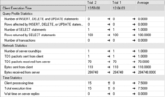
Although capturing client statistics can be a useful way to gather data, it's a limited set of data, and there is no way to show how one execution is different from another. You could even run a completely different query, and its data would be mixed in with the others, making the averages useless. If you need to, you can reset the client statistics. Select the Query menu and then the Reset Client Statistics menu item.
Both Duration and CPU represent the time factor of a query. To obtain detailed information on the amount of time (in milliseconds) required to parse, compile, and execute a query, use SET STATISTICS TIME as follows (timestats.sql in the download):
SET STATISTICS TIME ON
GO
SELECT  soh.AccountNumber,
        sod.LineTotal,
        sod.OrderQty,
        sod.UnitPrice,
        p.Name
FROM    Sales.SalesOrderHeader soh
        JOIN Sales.SalesOrderDetail sod
        ON soh.SalesOrderID = sod.SalesOrderID
        JOIN Production.Product p
        ON sod.ProductID = p.ProductID
WHERE   sod.LineTotal > 1000 ;
GO
SET STATISTICS TIME OFF
GO
The output of STATISTICS TIME for the preceding SELECT statement is as follows:
SQL Server parse and compile time:
    CPU time = 0 ms, elapsed time = 0 ms.

(32101 row(s) affected)

 SQL Server Execution Times:
   CPU time = 140 ms,  elapsed time = 763 ms.
 SQL Server parse and compile time:
     CPU time = 0 ms, elapsed time = 0 ms.
The CPU time = 140 ms part of the execution times represents the CPU value provided by the Profiler tool and the Server Trace option. Similarly, the corresponding Elapsed time = 763 ms represents the Duration value provided by the other mechanisms.
A 0 ms parse and compile time signifies that the optimizer reused the existing execution plan for this query and therefore didn't have to spend any time parsing and compiling the query again. If the query is executed for the first time, then the optimizer has to parse the query first for syntax and then compile it to produce the execution plan. This can be easily verified by clearing out the cache using the system call DBCC FREEPROCCACHE and then rerunning the query:
SQL Server parse and compile time:
   CPU time = 32 ms, elapsed time = 39 ms.

(162 row(s) affected)

 SQL Server Execution Times:
   CPU time = 187 ms,  elapsed time = 699 ms.
SQL Server parse and compile time:
   CPU time = 0 ms, elapsed time = 0 ms.
This time, SQL Server spent 32 ms of CPU time and a total of 39 ms parsing and compiling the query.
Note
You should not run DBCC FREEPROCCACHE on your production systems unless you are prepared to incur the not insignificant cost of recompiling every query on the system. In some ways, this will be as costly to your system as a reboot.
As discussed in the "Identifying Costly Queries" section earlier in the chapter, the number of reads in the Reads column is frequently the most significant cost factor among Duration, CPU, Reads, and Writes. The total number of reads performed by a query consists of the sum of the number of reads performed on all tables involved in the query. The reads performed on the individual tables may vary significantly, depending on the size of the result set requested from the individual table and the indexes available.
To reduce the total number of reads, it will be useful to find all the tables accessed in the query and their corresponding number of reads. This detailed information helps you concentrate on optimizing data access on the tables with a large number of reads. The number of reads per table also helps you evaluate the impact of the optimization step (implemented for one table) on the other tables referred to in the query.
In a simple query, you determine the individual tables accessed by taking a close look at the query. This becomes increasingly difficult the more complex the query becomes. In the case of a stored procedure, database views, or functions, it becomes more difficult to identify all the tables actually accessed by the optimizer. You can use STATISTICS IO to get this information, irrespective of query complexity.
To turn STATISTICS IO on, navigate to Query
SET STATISTICS IO ON
GO
SELECT  soh.AccountNumber,
        sod.LineTotal,
        sod.OrderQty,
        sod.UnitPrice,
        p.Name
FROM    Sales.SalesOrderHeader soh
        JOIN Sales.SalesOrderDetail sod
        ON soh.SalesOrderID = sod.SalesOrderID
        JOIN Production.Product p
        ON sod.ProductID = p.ProductID
WHERE   sod.SalesOrderId = 71856;
GO
SET STATISTICS IO OFF
GO
If you run this query and look at the execution plan, it consists of three clustered index seeks with two loop joins. If you remove the WHERE clause and run the query again, you get a set of scans and some hash joins. That's an interesting fact—but you don't know how it affects the query cost! You can use SET STATISTICS IO as shown previously to compare the cost of the query (in terms of logical reads) between the two processing strategies used by the optimizer.
You get following STATISTICS IO output when the query uses the hash join:
Table 'Worktable'. Scan count 0, logical reads 0, physical reads 0...
Table 'SalesOrderDetail'. Scan count 1, logical reads 1240, physical reads 0...
Table 'SalesOrderHeader'. Scan count 1, logical reads 686, physical reads 0...
Table 'Product'. Scan count 1, logical reads 5, physical reads 0...
Now when you add the WHERE clause to appropriately filter the data, the resultant STATISTICS IO output turns out to be this:
Table 'Product'. Scan count 0, logical reads 4, physical reads 0...
Table 'SalesOrderDetail'. Scan count 1, logical reads 3, physical reads 0...
Table 'SalesOrderHeader'. Scan count 0, logical reads 3, physical reads 0...
Logical reads for the SalesOrderDetail table have been cut from 1,240 to 3 because of the index seek and the loop join. It also hasn't significantly affected the data retrieval cost of the Product table.
While interpreting the output of STATISTICS IO, you mostly refer to the number of logical reads. Sometimes you also refer to the scan count, but even if you perform few logical reads per scan, the total number of logical reads provided by STATISTICS IO can still be high. If the number of logical reads per scan is small for a specific table, then you may not be able to improve the indexing mechanism of the table any further. The number of physical reads and read-ahead reads will be nonzero when the data is not found in the memory, but once the data is populated in memory, the physical reads and read-ahead reads will tend to be zero.
There is another advantage to knowing all the tables used and their corresponding reads for a query. Both the Duration and CPU values may fluctuate significantly when reexecuting the same query with no change in table schema (including indexes) or data because the essential services and background applications running on the SQL Server machine usually affect the processing time of the query under observation.
During optimization steps, you need a nonfluctuating cost figure as a reference. The reads (or logical reads) don't vary between multiple executions of a query with a fixed table schema and data. For example, if you execute the previous SELECT statement ten times, you will probably get ten different figures for Duration and CPU, but Reads will remain the same each time. Therefore, during optimization, you can refer to the number of reads for an individual table to ensure that you really have reduced the data access cost of the table.
Even though the number of logical reads can also be obtained from Profiler or the Server Trace option, you get another benefit when using STATISTICS IO. The number of logical reads for a query shown by Profiler or the Server Trace option increases as you use different SET statements (mentioned previously) along with the query. But the number of logical reads shown by STATISTICS IO doesn't include the additional pages that are accessed as SET statements are used with a query. Thus, STATISTICS IO provides a consistent figure for the number of logical reads.
In this chapter, you saw that you can use the Profiler tool or SQL tracing to identify the queries causing a high amount of stress on the system resources in a SQL workload. Collecting the trace data can, and should be, automated using system stored procedures. For immediate access to statistics about running queries, use the DMV sys.dm_exec_query_stats. You can further analyze these queries with Management Studio to find the costly steps in the processing strategy of the query. For better performance, it is important to consider both the index and join mechanisms used in an execution plan while analyzing a query. The number of data retrievals (or reads) for the individual tables provided by SET STATISTICS IO helps concentrate on the data access mechanism of the tables with most number of reads. You also should focus on the CPU cost and overall time of the most costly queries.
Once you identify a costly query and finish the initial analysis, the next step should be to optimize the query for performance. Because indexing is one of the most commonly used performance-tuning techniques, in the next chapter I will discuss in depth the various indexing mechanisms available in SQL Server.