
![]()
This book is about improving the performance of .NET applications. You can’t improve something that you can’t measure first, which is why our first substantial chapter deals with performance measurement tools and techniques. Guessing where the application’s bottlenecks are and jumping to premature conclusions on what to optimize is the worst thing a performance-conscious developer can do and often ends perilously. As we have seen in Chapter 1, there are many interesting performance metrics that can be the central factor to your application’s perceived performance; in this chapter we shall see how to obtain them.
Approaches to Performance Measurement
There is more than one right way to measure application performance, and much depends on the context, the application’s complexity, the type of information required, and the accuracy of the obtained results.
One approach for testing small programs or library methods is white-box testing: inspecting source code, analyzing its complexity on the whiteboard, modifying the program’s source, and inserting measurement code in it. We will discuss this approach, often called microbenchmarking, towards the end of this chapter; it can be very valuable—and often irreplaceable—where precise results and absolute understanding of every CPU instruction is required, but rather time-consuming and inflexible where large applications are concerned. Additionally, if you don’t know in advance which small part of the program to measure and reason about, isolating the bottleneck can be extremely difficult without resorting to automatic tools.
For larger programs, the more common approach is black-box testing, where a performance metric is identified by a human and then measured automatically by a tool. When using this approach, the developer doesn’t have to identify the performance bottleneck in advance, or assume that the culprit is in a certain (and small) part of the program. Throughout this chapter we will consider numerous tools that analyze the application’s performance automatically and present quantitative results in an easily digestible form. Among these tools are performance counters, Event Tracing for Windows (ETW), and commercial profilers.
As you read this chapter, bear in mind that performance measurement tools can adversely affect application performance. Few tools can provide accurate information and at the same time present no overhead when the application is executing. As we move from one tool to the next, always remember that the accuracy of the tools is often at conflict with the overhead they inflict upon your application.
Before we turn to commercial tools that tend to require installation and intrusively measure your application’s performance, it’s paramount to make sure everything Windows has to offer out-of-the-box has been used to its fullest extent. Performance counters have been a part of Windows for nearly two decades, whereas Event Tracing for Windows is slightly newer and has become truly useful around the Windows Vista time frame (2006). Both are free, present on every edition of Windows, and can be used for performance investigations with minimal overhead.
Performance Counters
Windows performance counters are a built-in Windows mechanism for performance and health investigation. Various components, including the Windows kernel, drivers, databases, and the CLR provide performance counters that users and administrators can consume and understand how well the system is functioning. As an added bonus, performance counters for the vast majority of system components are turned on by default, so you will not be introducing any additional overhead by collecting this information.
Reading performance counter information from a local or remote system is extremely easy. The built-in Performance Monitor tool (perfmon.exe) can display every performance counter available on the system, as well as log performance counter data to a file for subsequent investigation and provide automatic alerts when performance counter readings breach a defined threshold. Performance Monitor can monitor remote systems as well, if you have administrator permissions and can connect to them through a local network.
Performance information is organized in the following hierarchy:
- Performance counter categories (or performance objects) represent a set of individual counters related to a certain system component. Some examples of categories include .NET CLR Memory, Processor Information, TCPv4, and PhysicalDisk.
- Performance counters are individual numeric data properties in a performance counter category. It is common to specify the performance counter category and performance counter name separated by a slash, e.g., ProcessPrivate Bytes. Performance counters have several supported types, including raw numeric information (ProcessThread Count), rate of events (Print QueueBytes Printed/sec), percentages (PhysicalDisk\% Idle Time), and averages (ServiceModelOperation 3.0.0.0Calls Duration).
- Performance counter category instances are used to distinguish several sets of counters from a specific component of which there are several instances. For example, because there may be multiple processors on a system, there is an instance of the Processor Information category for each processor (as well as an aggregated _Total instance). Performance counter categories can be multi-instance—and many are—or single-instance (such as the Memory category).
If you examine the full list of performance counters provided by a typical Windows system that runs .NET applications, you’ll see that many performance problems can be identified without resorting to any other tool. At the very least, performance counters can often provide a general idea of which direction to pursue when investigating a performance problem or inspecting data logs from a production system to understand if it’s behaving normally.
Below are some scenarios in which a system administrator or performance investigator can obtain a general idea of where the performance culprit lies before using heavier tools:
- If an application exhibits a memory leak, performance counters can be used to determine whether managed or native memory allocations are responsible for it. The ProcessPrivate Bytes counter can be correlated with the .NET CLR Memory# Bytes in All Heaps counter. The former accounts for all private memory allocated by the process (including the GC heap) whereas the latter accounts only for managed memory. (See Figure 2-1.)
- If an ASP.NET application starts exhibiting abnormal behavior, the ASP.NET Applications category can provide more insight into what’s going on. For example, the Requests/Sec, Requests Timed Out, Request Wait Time, and Requests Executing counters can identify extreme load conditions, the Errors Total/Sec counter can suggest whether the application is facing an unusual number of exceptions, and the various cache- and output cache-related counters can indicate whether caching is being applied effectively.
- If a WCF service that heavily relies on a database and distributed transactions is failing to handle its current load, the ServiceModelService category can pinpoint the problem—the Calls Outstanding, Calls Per Second, and Calls Failed Per Second counters can identify heavy load, the Transactions Flowed Per Second counter reports the number of transactions the service is dealing with, and at the same time SQL Server categories such as MSSQL$INSTANCENAME:Transactions and MSSQL$INSTANCENAME:Locks can point to problems with transactional execution, excessive locking, and even deadlocks.
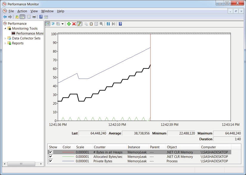
Figure 2-1 . The Performance Monitor main window, showing three counters for a specific process. The top line on the graph is the ProcessPrivate Bytes counter, the middle one is .NET CLR Memory# Bytes in all Heaps, and the bottom one is .NET CLR MemoryAllocated Bytes/sec. From the graph it is evident that the application exhibits a memory leak in the GC heap
MONITORING MEMORY USAGE WITH PERFORMANCE COUNTERS
In this short experiment, you will monitor the memory usage of a sample application and determine that it exhibits a memory leak using Performance Monitor and the performance counters discussed above.
- Open Performance Monitor—you can find it in the Start menu by searching for “Performance Monitor” or run perfmon.exe directly.
- Run the MemoryLeak.exe application from this chapter’s source code folder.
- Click the “Performance Monitor” node in the tree on the left, and then click the green + button.
- From the .NET CLR Memory category, select the # Bytes in all Heaps and Allocated Bytes/sec performance counters, select the MemoryLeak instance from the instance list, and click the “Add >>” button.
- From the Process category, select the Private Bytes performance counter, select the MemoryLeak instance from the instance list, and click the “Add >>” button.
- Click the “OK” button to confirm your choices and view the performance graph.
- You might need to right click the counters in the bottom part of the screen and select “Scale selected counters” to see actual lines on the graph.
![]() Tip There are literally thousands of performance counters on a typical Windows system; no performance investigator is expected to remember them all. This is where the small “Show description” checkbox at the bottom of the “Add Counters” dialog comes in handy—it can tell you that SystemProcessor Queue Length represents the number of ready threads waiting for execution on the system’s processors, or that .NET CLR LocksAndThreadsContention Rate / sec is the number of times (per second) that threads attempted to acquire a managed lock unsuccessfully and had to wait for it to become available.
Tip There are literally thousands of performance counters on a typical Windows system; no performance investigator is expected to remember them all. This is where the small “Show description” checkbox at the bottom of the “Add Counters” dialog comes in handy—it can tell you that SystemProcessor Queue Length represents the number of ready threads waiting for execution on the system’s processors, or that .NET CLR LocksAndThreadsContention Rate / sec is the number of times (per second) that threads attempted to acquire a managed lock unsuccessfully and had to wait for it to become available.
Performance Counter Logs and Alerts
Configuring performance counter logs is fairly easy, and you can even provide an XML template to your system administrators to apply performance counter logs automatically without having to specify individual performance counters. You can open the resulting logs on any machine and play them back as if they represent live data. (There are even some built-in counter sets you can use instead of configuring what data to log manually.)
You can also use Performance Monitor to configure a performance counter alert, which will execute a task when a certain threshold is breached. You can use performance counter alerts to create a rudimentary monitoring infrastructure, which can send an email or message to a system administrator when a performance constraint is violated. For example, you could configure a performance counter alert that would automatically restart your process when it reaches a dangerous amount of memory usage, or when the system as a whole runs out of disk space. We strongly recommend that you experiment with Performance Monitor and familiarize yourself with the various options it has to offer.
CONFIGURING PERFORMANCE COUNTER LOGS
To configure performance counter logs, open Performance Monitor and perform the following steps. (We assume that you are using Performance Monitor on Windows 7 or Windows Server 2008 R2; in prior operating system versions, Performance Monitor had a slightly different user interface—if you are using these versions, consult the documentation for detailed instructions.)
- In the tree on the left, expand the Data Collector Sets node.
- Right-click the User Defined node and select New
 Data Collector Set from the context menu.
 - Name your data collector set, select the “Create manually (Advanced)” radio button, and click Next.
- Make sure the “Create data logs” radio button is selected, check the “Performance counter” checkbox, and click Next.
- Use the Add button to add performance counters (the standard Add Counters dialog will open). When you’re done, configure a sample interval (the default is to sample the counters every 15 seconds) and click Next.
- Provide a directory which Performance Monitor will use to store your counter logs and then click Next.
- Select the “Open properties for this data collector set” radio button and click Finish.
- Use the various tabs to further configure your data collector set—you can define a schedule for it to run automatically, a stop condition (e.g. after collecting more than a certain amount of data), and a task to run when the data collection stops (e.g. to upload the results to a centralized location). When you’re done, click OK.
- Click the User Defined node, right-click your data collector set in the main pane, and select Start from the context menu.
- Your counter log is now running and collecting data to the directory you’ve selected. You can stop the data collector set at any time by right-clicking it and selecting Stop from the context menu.
When you’re done collecting the data and want to inspect it using the Performance Monitor, perform the following steps:
- Select the User Defined node.
- Right-click your data collector set and select Latest Report from the context menu.
- In the resulting window, you can add or delete counters from the list of counters in the log, configure a time range and change the data scale by right-clicking the graph and selecting Properties from the context menu.
Custom Performance Counters
Although Performance Monitor is an extremely useful tool, you can read performance counters from any .NET application using the System.Diagnostics.PerformanceCounter class. Even better, you can create your own performance counters and add them to the vast set of data available for performance investigation.
Below are some scenarios in which you should consider exporting performance counter categories:
- You are developing an infrastructure library to be used as part of large systems. Your library can report performance information through performance counters, which is often easier on developers and system administrators than following log files or debugging at the source code level.
- You are developing a server system which accepts custom requests, processes them, and delivers responses (custom Web server, Web service, etc.). You should report performance information for the request processing rate, errors encountered, and similar statistics. (See the ASP.NET performance counter categories for some ideas.)
- You are developing a high-reliability Windows service that runs unattended and communicates with custom hardware. Your service can report the health of the hardware, the rate of your software’s interactions with it, and similar statistics.
The following code is all it takes to export a single-instance performance counter category from your application and to update these counters periodically. It assumes that the AttendanceSystem class has information on the number of employees currently signed in, and that you want to expose this information as a performance counter. (You will need the System.Diagnostics namespace to compile this code fragment.)
public static void CreateCategory() {
  if (PerformanceCounterCategory.Exists("Attendance")) {
   PerformanceCounterCategory.Delete("Attendance");
  }
  CounterCreationDataCollection counters = new CounterCreationDataCollection();
  CounterCreationData employeesAtWork = new CounterCreationData(
   "# Employees at Work", "The number of employees currently checked in.",
   PerformanceCounterType.NumberOfItems32);
  PerformanceCounterCategory.Create(
   "Attendance", "Attendance information for Litware, Inc.",
   PerformanceCounterCategoryType.SingleInstance, counters);
}
public static void StartUpdatingCounters() {
  PerformanceCounter employeesAtWork = new PerformanceCounter(
   "Attendance", "# Employees at Work", readOnly: false);
  updateTimer = new Timer(_ = > {
   employeesAtWork.RawValue = AttendanceSystem.Current.EmployeeCount;
  }, null, TimeSpan.Zero, TimeSpan.FromSeconds(1));
}
As we have seen, it takes very little effort to configure custom performance counters, and they can be of utmost importance when carrying out a performance investigation. Correlating system performance counter data with custom performance counters is often all a performance investigator needs to pinpoint the precise cause of a performance or configuration issue.
![]() Note Performance Monitor can be used to collect other types of information that have nothing to do with performance counters. You can use it to collect configuration data from a system—the values of registry keys, WMI objects properties, and even interesting disk files. You can also use it to capture data from ETW providers (which we discuss next) for subsequent analysis. By using XML templates, system administrators can quickly apply data collector sets to a system and generate a useful report with very few manual configuration steps.
Note Performance Monitor can be used to collect other types of information that have nothing to do with performance counters. You can use it to collect configuration data from a system—the values of registry keys, WMI objects properties, and even interesting disk files. You can also use it to capture data from ETW providers (which we discuss next) for subsequent analysis. By using XML templates, system administrators can quickly apply data collector sets to a system and generate a useful report with very few manual configuration steps.
Although performance counters offer a great amount of interesting performance information, they cannot be used as a high-performance logging and monitoring framework. There are no system components that update performance counters more often than a few times a second, and the Windows Performance Monitor won’t read performance counters more often than once a second. If your performance investigation requires following thousands of events per second, performance counters are not a good fit. We now turn our attention to Event Tracing for Windows (ETW), which was designed for high-performance data collection and richer data types (not just numbers).
Event Tracing for Windows (ETW)
Event Tracing for Windows (ETW) is a high-performance event logging framework built into Windows. As was the case with performance counters, many system components and application frameworks, including the Windows kernel and the CLR, define providers, which report events—information on the component’s inner workings. Unlike performance counters, that are always on, ETW providers can be turned on and off at runtime so that the performance overhead of transferring and collecting them is incurred only when they’re needed for a performance investigation.
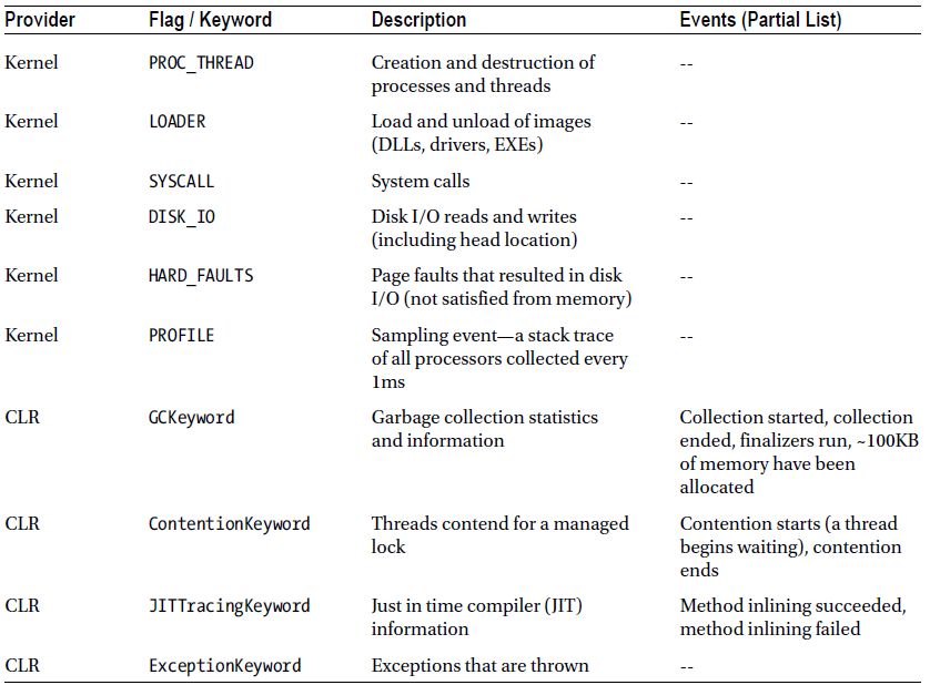
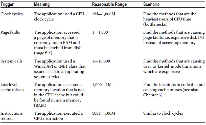
One of the richest sources of ETW information is the kernel provider, which reports events on process and thread creation, DLL loading, memory allocation, network I/O, and stack trace accounting (also known as sampling). Table 2-1 shows some of the useful information reported by the kernel and CLR ETW providers. You can use ETW to investigate overall system behavior, such as what processes are consuming CPU time, to analyze disk I/O and network I/O bottlenecks, to obtain garbage collection statistics and memory usage for managed processes, and many other scenarios discussed later in this section.
ETW events are tagged with a precise time and can contain custom information, as well as an optional stack trace of where they occurred. These stack traces can be used to further identify sources of performance and correctness problems. For example, the CLR provider can report events at the start and end of every garbage collection. Combined with precise call stacks, these events can be used to determine which parts of the program are typically causing garbage collection. (For more information about garbage collection and its triggers, see Chapter 4.)
Table 2-1. Partial List of ETW Events in Windows and the CLR
Accessing this highly detailed information requires an ETW collection tool and an application that can read raw ETW events and perform some basic analysis. At the time of writing, there were two tools capable of both tasks: Windows Performance Toolkit (WPT, also known as XPerf), which ships with the Windows SDK, and PerfMonitor (do not confuse it with Windows Performance Monitor!), which is an open source project by the CLR team at Microsoft.
Windows Performance Toolkit (WPT)
Windows Performance Toolkit (WPT) is a set of utilities for controlling ETW sessions, capturing ETW events into log files, and processing them for later display. It can generate graphs and overlays of ETW events, summary tables including call stack information and aggregation, and CSV files for automated processing. To download WPT, download the Windows SDK Web installer from http://msdn.microsoft.com/en-us/performance/cc752957.aspx and select only Common Utilities ![]() Windows Performance Toolkit from the installation options screen. After the Windows SDK installer completes, navigate to the RedistWindows Performance Toolkit subdirectory of the SDK installation directory and run the installer file for your system’s architecture (Xperf_x86.msi for 32-bit systems, Xperf_x64.msi for 64-bit systems).
Windows Performance Toolkit from the installation options screen. After the Windows SDK installer completes, navigate to the RedistWindows Performance Toolkit subdirectory of the SDK installation directory and run the installer file for your system’s architecture (Xperf_x86.msi for 32-bit systems, Xperf_x64.msi for 64-bit systems).
![]() Note On 64-bit Windows, stack walking requires changing a registry setting that disables paging-out of kernel code pages (for the Windows kernel itself and any drivers). This may increase the system’s working set (RAM utilization) by a few megabytes. To change this setting, navigate to the registry key HKLMSystemCurrentControlSetControlSession ManagerMemory Management, set the DisablePagingExecutive value to the DWORD 0x1, and restart the system.
Note On 64-bit Windows, stack walking requires changing a registry setting that disables paging-out of kernel code pages (for the Windows kernel itself and any drivers). This may increase the system’s working set (RAM utilization) by a few megabytes. To change this setting, navigate to the registry key HKLMSystemCurrentControlSetControlSession ManagerMemory Management, set the DisablePagingExecutive value to the DWORD 0x1, and restart the system.
The tools you’ll use for capturing and analyzing ETW traces are XPerf.exe and XPerfView.exe. Both tools require administrative privileges to run. The XPerf.exe tool has several command line options that control which providers are enabled during the trace, the size of the buffers used, the file name to which the events are flushed, and many additional options. The XPerfView.exe tool analyzes and provides a graphical report of what the trace file contains.
All traces can be augmented with call stacks, which often allow precise zooming-in on the performance issues. However, you don’t have to capture events from a specific provider to obtain stack traces of what the system is doing; the SysProfile kernel flag group enables collection of stack traces from all processors captured at 1ms intervals. This is a rudimentary way of understanding what a busy system is doing at the method level. (We’ll return to this mode in more detail when discussing sampling profilers later in this chapter.)
CAPTURING AND ANALYZING KERNEL TRACES WITH XPERF
In this section, you’ll capture a kernel trace using XPerf.exe and analyze the results in the XPerfView.exe graphical tool. This experiment is designed to be carried out on Windows Vista system or a later version. (It also requires you to set two system environment variables. To do so, right click Computer, click Properties, click “Advanced system settings” and finally click the “Environment Variables” button at the bottom of the dialog.)
- Set the system environment variable _NT_SYMBOL_PATH to point to the Microsoft public symbol server and a local symbol cache, e.g.: srv*C:TempSymbols*http://msdl.microsoft.com/download/symbols
- Set the system environment variable _NT_SYMCACHE_PATH to a local directory on your disk—this should be a different directory from the local symbols cache in the previous step.
- Open an administrator Command Prompt window and navigate to the installation directory where you installed WPT (e.g. C:Program FilesWindows Kits8.0Windows Performance Toolkit).
- Begin a trace with the Base kernel provider group, which contains the PROC_THREAD, LOADER, DISK_IO, HARD_FAULTS, PROFILE, MEMINFO, and MEMINFO_WS kernel flags (see Table 2-1). To do this, run the following command: xperf -on Base
- Initiate some system activity: run applications, switch between windows, open files—for at least a few seconds. (These are the events that will enter the trace.)
- Stop the trace and flush the trace to a log file by running the following command: xperf -d KernelTrace.etl
- Launch the graphical performance analyzer by running the following command: xperfview KernelTrace.etl
- The resulting window contains several graphs, one for each ETW keyword that generated events during the trace. You can choose the graphs to display on the left. Typically, the topmost graph displays the processor utilization by processor, and subsequent graphs display the disk I/O operation count, memory usage, and other statistics.
- Select a section of the processor utilization graph, right click it, and select Load Symbols from the context menu. Right click the selected section again, and select Simple Summary Table. This should open an expandable view in which you can navigate between methods in all processes that had some processor activity during the trace. (Loading the symbols from the Microsoft symbol server for the first time can be time consuming.)
There are many useful scenarios in which WPT can provide insight into the system’s overall behavior and the performance of individual processes. Below are some screenshots and examples of these scenarios:
- WPT can capture all disk I/O operations on a system and display them on a map of the physical disk. This provides insight into expensive I/O operations, especially where large seeks are involved on rotating hard drives. (See Figure 2-2.)
- WPT can provide call stacks for all processor activity on the system during the trace. It aggregates call stacks at the process, module, and function level, and allows at-a-glance understanding of where the system (or a specific application) is spending CPU time. Note that managed frames are not supported—we’ll address this deficiency later with the PerfMonitor tool. (See Figure 2-3.)
- WPT can display overlay graphs of different activity types to provide correlation between I/O operations, memory utilization, processor activity, and other captured metrics. (See Figure 2-4.)
- WPT can display call stack aggregations in a trace (when the trace is initially configured with the -stackwalk command line switch)—this provides complete information on call stacks which created certain events. (See Figure 2-5.)
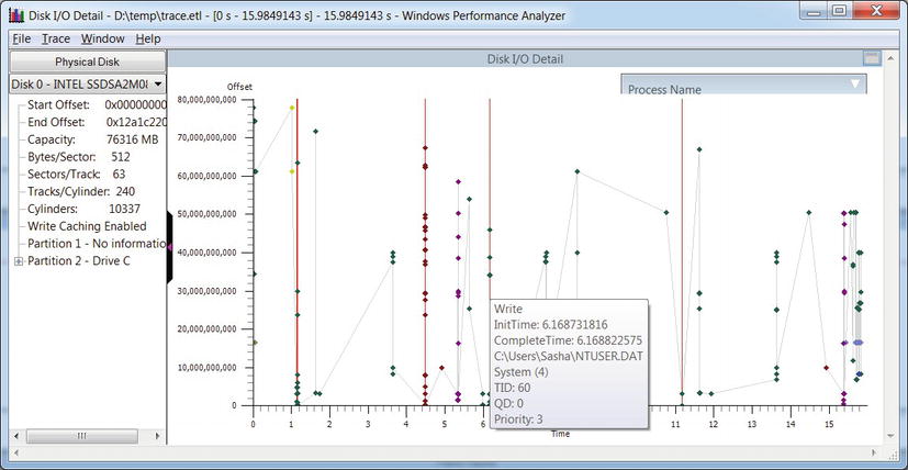
Figure 2-2 . Disk I/O operations laid out on a map of the physical disk. Seeks between I/O operations and individual I/O details are provided through tooltips
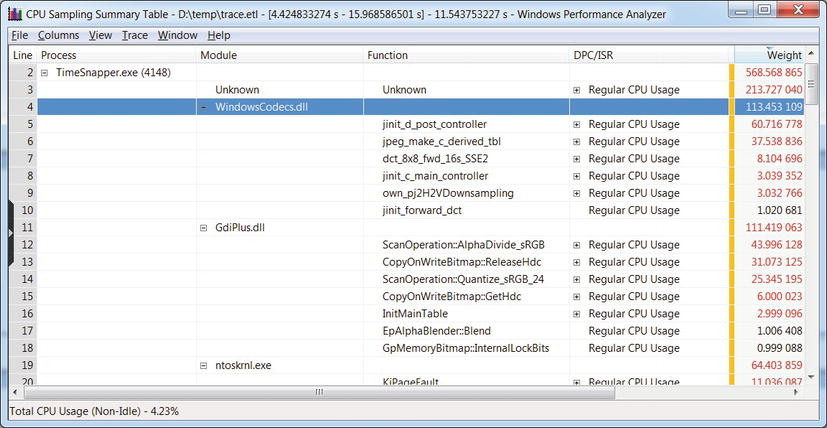
Figure 2-3 . Detailed stack frames for a single process (TimeSnapper.exe). The Weight column indicates (roughly) how much CPU time was spent in that frame
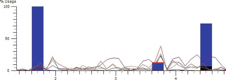
Figure 2-4 . Overlay graph of CPU activity (lines—each line indicates a different processor) and disk I/O operations (columns). No explicit correlation between I/O activity and CPU activity is visible
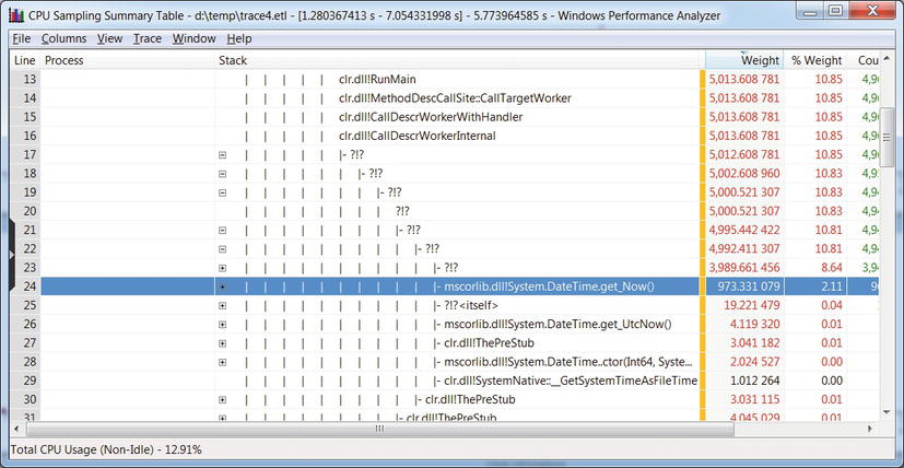
Figure 2-5 . Call stack aggregation in the report. Note that managed frames are displayed only partially—the ?!? frames could not be resolved. The mscorlib.dll frames (e.g. System.DateTime.get_Now()) were resolved successfully because they are pre-compiled using NGen and not compiled by the JIT compiler at runtime
![]() Note The latest version of the Windows SDK (version 8.0) ships with a pair of new tools, called Windows Performance Recorder (wpr.exe) and Windows Performance Analyzer (wpa.exe), that were designed to gradually replace the XPerf and XPerfView tools we used earlier. For example, wpr -start CPU is roughly equivalent to xperf -on Diag, and wpr -stop reportfile is roughly equivalent to xperf -d reportfile. The WPA analysis UI is slightly different, but provides features similar to XPerfView. For more information on the new tools, consult the MSDN documentation at http://msdn.microsoft.com/en-us/library/hh162962.aspx.
Note The latest version of the Windows SDK (version 8.0) ships with a pair of new tools, called Windows Performance Recorder (wpr.exe) and Windows Performance Analyzer (wpa.exe), that were designed to gradually replace the XPerf and XPerfView tools we used earlier. For example, wpr -start CPU is roughly equivalent to xperf -on Diag, and wpr -stop reportfile is roughly equivalent to xperf -d reportfile. The WPA analysis UI is slightly different, but provides features similar to XPerfView. For more information on the new tools, consult the MSDN documentation at http://msdn.microsoft.com/en-us/library/hh162962.aspx.
XPerfView is very capable of displaying kernel provider data in attractive graphs and tables, but its support for custom providers is not as powerful. For example, we can capture events from the CLR ETW provider, but XPerfView will not generate pretty graphs for the various events—we’ll have to make sense of the raw data in the trace based on the list of keywords and events in the provider’s documentation (the full list of the CLR ETW provider’s keywords and events is available in the MSDN documentation—http://msdn.microsoft.com/en-us/library/ff357720.aspx).
If we run XPerf with the CLR ETW provider (e13c0d23-ccbc-4e12-931b-d9cc2eee27e4) the keyword for GC events (0x00000001), and the Verbose log level (0x5), it will dutifully capture every event the provider generates. By dumping it to a CSV file or opening it with XPerfView we will be able—slowly—to identify GC-related events in our application. Figure 2-6 shows a sample of the resulting XPerfView report—the time elapsed between the GC /Start and GC /Stop rows is the time it took a single garbage collection to complete in the monitored application.
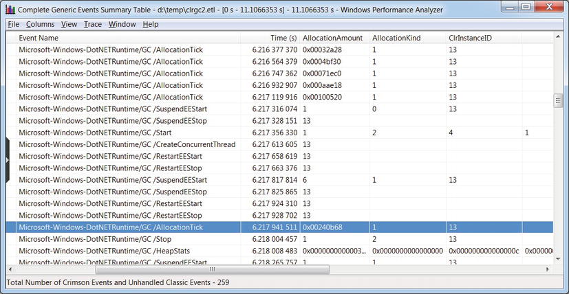
Figure 2-6 . Raw report of CLR GC-related events. The selected row displays the GCAllocationTick_V1 event that is raised every time approximately 100KB of memory is allocated
Fortunately, the Base Class Library (BCL) team at Microsoft has identified this deficiency and provided an open source library and tool for analyzing CLR ETW traces, called PerfMonitor. We discuss this tool next.
The PerfMonitor.exe open source command line tool has been released by the BCL team at Microsoft through the CodePlex website. At the time of writing the latest release was PerfMonitor 1.5 that can be downloaded from http://bcl.codeplex.com/releases/view/49601. PerfMonitor’s primary advantage compared to WPT is that it has intimate knowledge about CLR events and provides more than just raw tabular data. PerfMonitor analyzes GC and JIT activity in the process, and can sample managed stack traces and determine which parts of the application are using CPU time.
For advanced users, PerfMonitor also ships with a library called TraceEvent, which enables programmatic access to CLR ETW traces for automatic inspection. You could use the TraceEvent library in custom system monitoring software to inspect automatically a trace from a production system and decide how to triage it.
Although PerfMonitor can be used to collect kernel events or even events from a custom ETW provider (using the /KernelEvents and /Provider command line switches), it is typically used to analyze the behavior of a managed application using the built-in CLR providers. Its runAnalyze command line option executes an application of your choice, monitors its execution, and upon its termination generates a detailed HTML report and opens it in your default browser. (You should follow the PerfMonitor user guide—at least through the Quick Start section—to generate reports similar to the screenshots in this section. To display the user guide, run PerfMonitor usersguide.)
When PerfMonitor is instructed to run an application and generate a report, it produces the following command line output. You can experiment with the tool yourself as you read this section by running it on the JackCompiler.exe sample application from this chapter’s source code folder.
C:PerfMonitor > perfmonitor runAnalyze JackCompiler.exe
Starting kernel tracing. Output file: PerfMonitorOutput.kernel.etl
Starting user model tracing. Output file: PerfMonitorOutput.etl
Starting at 4/7/2012 12:33:40 PM
Current Directory C:PerfMonitor
Executing: JackCompiler.exe {
} Stopping at 4/7/2012 12:33:42 PM = 1.724 sec
Stopping tracing for sessions 'NT Kernel Logger' and 'PerfMonitorSession'.
Analyzing data in C:PerfMonitorPerfMonitorOutput.etlx
GC Time HTML Report in C:PerfMonitorPerfMonitorOutput.GCTime.html
JIT Time HTML Report in C:PerfMonitorPerfMonitorOutput.jitTime.html
Filtering to process JackCompiler (1372). Started at 1372.000 msec.
Filtering to Time region [0.000, 1391.346] msec
CPU Time HTML report in C:PerfMonitorPerfMonitorOutput.cpuTime.html
Filtering to process JackCompiler (1372). Started at 1372.000 msec.
Perf Analysis HTML report in C:PerfMonitorPerfMonitorOutput.analyze.html
PerfMonitor processing time: 7.172 secs.
The various HTML files generated by PerfMonitor contain the distilled report, but you can always use the raw ETL files with XPerfView or any other tool that can read binary ETW traces. The summary analysis for the example above contains the following information (this might vary, of course, when you run this experiment on your own machine):
- CPU Statistics—CPU time consumed was 917ms and the average CPU utilization was 56.6%. The rest of the time was spent waiting for something.
- GC Statistics—the total GC time was 20ms, the maximum GC heap size was 4.5MB, the maximum allocation rate was 1496.1MB/s, and the average GC pause was 0.1ms.
- JIT Compilation Statistics—159 methods were compiled at runtime by the JIT compiler, for a total of 30493 bytes of machine code.
Drilling down to the CPU, GC, and JIT reports can provide a wealth of useful information. The CPU detailed report provides information on methods that use a large percentage of CPU time (bottom up analysis), a call tree of where CPU time is spent (top down analysis), and individual caller-callee views for each method in the trace. To prevent the report from growing very large, methods that do not exceed a predefined relevance threshold (1% for the bottom up analysis and 5% for the top down analysis) are excluded. Figure 2-7 is an example of a bottom up report—the three methods with most CPU work were System.String.Concat, JackCompiler.Tokenizer.Advance, and System.Linq.Enumerable.Contains. Figure 2-8 is an example of (part of) a top down report—84.2% of the CPU time is consumed by JackCompiler.Parser.Parse, which calls out to ParseClass, ParseSubDecls, ParseSubDecl, ParseSubBody, and so on.
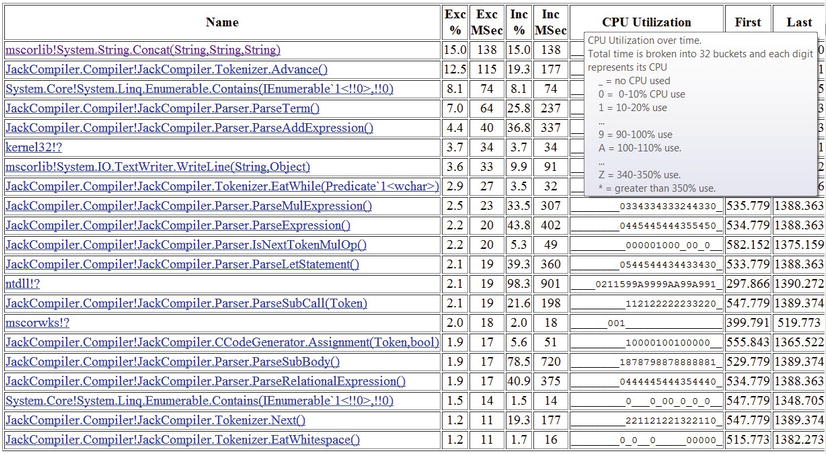
Figure 2-7 . Bottom up report from PerfMonitor. The “Exc %” column is an estimation of the CPU time used by that method alone; the “Inc %” column is an estimation of the CPU time used by that method and all other methods it called (its sub-tree in the call tree)
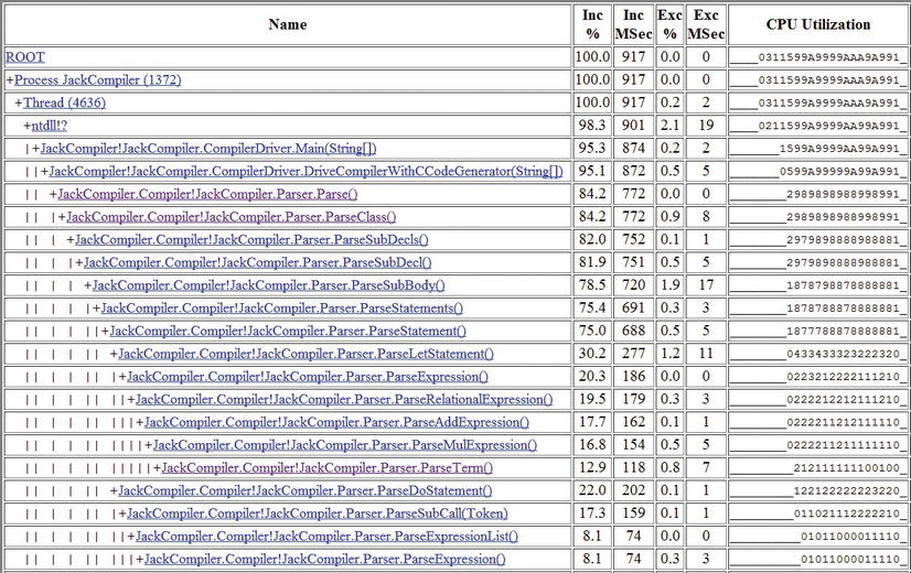
Figure 2-8 . Top down report from PerfMonitor
The detailed GC analysis report contains a table with garbage collection statistics (counts, times) for each generation, as well as individual GC event information, including pause times, reclaimed memory, and many others. Some of this information will be extremely useful when we discuss the garbage collector’s inner workings and performance implications in Chapter 4. Figure 2-9 shows a few rows for the individual GC events.

Figure 2-9 . Individual GC events, including the amount of memory reclaimed, the application pause time, the type of collection incurred, and other details
Finally, the detailed JIT analysis report shows how much time the JIT compiler required for each of the application’s methods as well as the precise time at which they were compiled. This information can be useful to determine whether application startup performance can be improved—if an excessive amount of startup time is spent in the JIT compiler, pre-compiling your application’s binaries (using NGen) may be a worthwhile optimization. We will discuss NGEN and other strategies for reducing application startup time in Chapter 10.
![]() Tip Collecting information from multiple high-performance ETW providers can generate very large log files. For example, in default collection mode PerfMonitor routinely generates over 5MB of raw data per second. Leaving such a trace on for several days is likely to exhaust disk space even on large hard drives. Fortunately, both XPerf and PerfMonitor support circular logging mode, where only the last N megabytes of logs are retained. In PerfMonitor, the /Circular command-line switch takes the maximum log file size (in megabytes) and discards the oldest logs automatically when the threshold is exceeded.
Tip Collecting information from multiple high-performance ETW providers can generate very large log files. For example, in default collection mode PerfMonitor routinely generates over 5MB of raw data per second. Leaving such a trace on for several days is likely to exhaust disk space even on large hard drives. Fortunately, both XPerf and PerfMonitor support circular logging mode, where only the last N megabytes of logs are retained. In PerfMonitor, the /Circular command-line switch takes the maximum log file size (in megabytes) and discards the oldest logs automatically when the threshold is exceeded.
Although PerfMonitor is a very powerful tool, its raw HTML reports and abundance of command-line options make it somewhat difficult to use. The next tool we’ll see offers very similar functionality to PerfMonitor and can be used in the same scenarios, but has a much more user-friendly interface to collecting and interpreting ETW information and will make some performance investigations considerably shorter.
PerfView is a free Microsoft tool that unifies ETW collection and analysis capabilities already available in PerfMonitor with heap analysis features that we will discuss later in conjunction with tools such as CLR Profiler and ANTS Memory Profiler. You can download PerfView from the Microsoft download center, at http://www.microsoft.com/download/en/details.aspx?id=28567. Note that you have to run PerfView as an administrator, because it requires access to the ETW infrastructure.
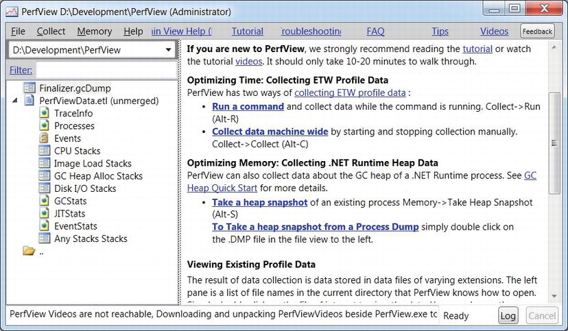
Figure 2-10 . PerfView’s main UI. In the file view (on the left) a heap dump and an ETW trace are visible. The links on the main view lead to various commands the tool supports
To analyze ETW information from a specific process, use the Collect ![]() Run menu item in PerfView (Figure 2-10 shows the main UI). For the purpose of the heap analysis we will perform shortly, you can use PerfView on the MemoryLeak.exe sample application from this chapter’s source code folder. It will run the process for you and generate a report with all the information PerfMonitor makes available and more, including:
Run menu item in PerfView (Figure 2-10 shows the main UI). For the purpose of the heap analysis we will perform shortly, you can use PerfView on the MemoryLeak.exe sample application from this chapter’s source code folder. It will run the process for you and generate a report with all the information PerfMonitor makes available and more, including:
- Raw list of ETW events collected from various providers (e.g. CLR contention information, native disk I/O, TCP packets, and hard page faults)
- Grouped stack locations where the application’s CPU time was spent, including configurable filters and thresholds
- Stack locations for image (assembly) loads, disk I/O operations, and GC allocations (for every ∼ 100KB of allocated objects)
- GC statistics and events, including the duration of each garbage collection and the amount of space reclaimed
Additionally, PerfView can be used to capture a heap snapshot from a currently running process or import a heap snapshot from a dump file. After importing, PerfView can be used to look for the types with most memory utilization in the snapshot and identify reference chains that are responsible for keeping these types alive. Figure 2-11 shows the PerfView reference analyzer for the Schedule class, which is responsible (inclusively) for 31MB of the heap snapshot’s contents. PerfView successfully identifies the Employee class instances holding references to Schedule objects, while Employee instances are being retained by the f-reachable queue (discussed in Chapter 4).

Figure 2-11 . Reference chain for Schedule class instances, responsible for 99.5% of the application’s memory usage in the captured heap snapshot
When we discuss memory profilers later in this chapter, we’ll see that PerfView’s visualization capabilities are still somewhat lacking compared to the commercial tools. Still, PerfView is a very useful free tool that can make many performance investigations significantly shorter. You can learn more about it using the built-in tutorial linked from its main screen, and there are also videos recorded by the BCL team that exhibit some of the tool’s main features.
Similarly to performance counters, you might want to tap into the powerful instrumentation and information collection framework offered by ETW for your own application’s needs. Prior to .NET 4.5, exposing ETW information from a managed application was fairly complex. You had to deal with plenty of details around defining a manifest for your application’s ETW provider, instantiating it at runtime, and logging events. As of .NET 4.5, writing a custom ETW provider could hardly be easier. All you need to do is derive from the System.Diagnostics.Tracing.EventSource class and call the WriteEvent base class method to output ETW events. All the details of registering an ETW provider with the system and formatting the event data are handled automatically for you.
The following class is an example of an ETW provider in a managed application (the full program is available in this chapter’s source code folder and you can run it with PerfMonitor later):
public class CustomEventSource : EventSource {
  public class Keywords {
   public const EventKeywords Loop = (EventKeywords)1;
   public const EventKeywords Method = (EventKeywords)2;
  }
  [Event(1, Level = EventLevel.Verbose, Keywords = Keywords.Loop,
   Message = "Loop {0} iteration {1}")]
  public void LoopIteration(string loopTitle, int iteration) {
   WriteEvent(1, loopTitle, iteration);
  }
  [Event(2, Level = EventLevel.Informational, Keywords = Keywords.Loop,
   Message = "Loop {0} done")]
  public void LoopDone(string loopTitle) {
   WriteEvent(2, loopTitle);
  }
  [Event(3, Level = EventLevel.Informational, Keywords = Keywords.Method,
   Message = "Method {0} done")]
  public void MethodDone([CallerMemberName] string methodName = null) {
   WriteEvent(3, methodName);
  }
}
class Program {
  static void Main(string[] args) {
   CustomEventSource log = new CustomEventSource();
   for (int i = 0; i < 10; ++i) {
   Thread.Sleep(50);
   log.LoopIteration("MainLoop", i);
   }
   log.LoopDone("MainLoop");
   Thread.Sleep(100);
   log.MethodDone();
  }
}
The PerfMonitor tool can be used to automatically obtain from this application the ETW provider it contains, run the application while monitoring that ETW provider, and generate a report of all ETW events the application submitted. For example:
C:PerfMonitor > perfmonitor monitorDump Ch02.exe
Starting kernel tracing. Output file: PerfMonitorOutput.kernel.etl
Starting user model tracing. Output file: PerfMonitorOutput.etl
Found Provider CustomEventSource Guid ff6a40d2-5116-5555-675b-4468e821162e
Enabling provider ff6a40d2-5116-5555-675b-4468e821162e level: Verbose keywords: 0xffffffffffffffff
Starting at 4/7/2012 1:44:00 PM
Current Directory C:PerfMonitor
Executing: Ch02.exe {
} Stopping at 4/7/2012 1:44:01 PM = 0.693 sec
Stopping tracing for sessions 'NT Kernel Logger' and 'PerfMonitorSession'.
Converting C:PerfMonitorPerfMonitorOutput.etlx to an XML file.
Output in C:PerfMonitorPerfMonitorOutput.dump.xml
PerfMonitor processing time: 1.886 secs.
![]() Note There is another performance monitoring and system health instrumentation framework we haven’t considered: Windows Management Instrumentation (WMI). WMI is a command-and-control (C&C) infrastructure integrated in Windows, and is outside the scope of this chapter. It can be used to obtain information about the system’s state (such as the installed operating system, BIOS firmware, or free disk space), register for interesting events (such as process creation and termination), and invoke control methods that change the system state (such as create a network share or unload a driver). For more information about WMI, consult the MSDN documentation at http://msdn.microsoft.com/en-us/library/windows/desktop/aa394582.aspx. If you are interested in developing managed WMI providers, Sasha Goldshtein’s article “WMI Provider Extensions in .NET 3.5” (http://www.codeproject.com/Articles/25783/WMI-Provider-Extensions-in-NET-3-5, 2008) provides a good start.
Note There is another performance monitoring and system health instrumentation framework we haven’t considered: Windows Management Instrumentation (WMI). WMI is a command-and-control (C&C) infrastructure integrated in Windows, and is outside the scope of this chapter. It can be used to obtain information about the system’s state (such as the installed operating system, BIOS firmware, or free disk space), register for interesting events (such as process creation and termination), and invoke control methods that change the system state (such as create a network share or unload a driver). For more information about WMI, consult the MSDN documentation at http://msdn.microsoft.com/en-us/library/windows/desktop/aa394582.aspx. If you are interested in developing managed WMI providers, Sasha Goldshtein’s article “WMI Provider Extensions in .NET 3.5” (http://www.codeproject.com/Articles/25783/WMI-Provider-Extensions-in-NET-3-5, 2008) provides a good start.
Although performance counters and ETW events offer a great amount of insight into the performance of Windows applications, there’s often a lot to be gained from more intrusive tools—profilers—that inspect application execution time at the method and line level (improving upon ETW stack trace collection support). In this section we introduce some commercial tools and see the benefits they bring to the table, bearing in mind that more powerful and accurate tools sustain a bigger measurement overhead.
Throughout our journey into the profiler world we will encounter numerous commercial tools; most of them have several readily available equivalents. We do not endorse any specific tool vendor; the products demonstrated in this chapter are simply the profilers we use most often and keep in our toolbox for performance investigations. As always with software tools, your mileage may vary.
The first profiler we consider is part of Visual Studio, and has been offered by Microsoft since Visual Studio 2005 (Team Suite edition). In this chapter, we’ll use the Visual Studio 2012 profiler, which is available in the Premium and Ultimate editions of Visual Studio.
Visual Studio Sampling Profiler
The Visual Studio sampling profiler operates similarly to the PROFILE kernel flag we’ve seen in the ETW section. It periodically interrupts the application and records the call stack information on every processor where the application’s threads are currently running. Unlike the kernel ETW provider, this sampling profiler can interrupt processes based on several criteria, some of which are listed in Table 2-2.
Table 2-2. Visual Studio Sampling Profiler Events (Partial List)
Capturing samples using the Visual Studio profiler is quite cheap, and if the sample event interval is wide enough (the default is 10,000,000 clock cycles), the overhead on the application’s execution can be less than 5%. Moreover, sampling is very flexible and enables attaching to a running process, collecting sample events for a while, and then disconnecting from the process to analyze the data. Because of these traits, sampling is the recommended approach to begin a performance investigation for CPU bottlenecks—methods that take a significant amount of CPU time.
When a sampling session completes, the profiler makes available summary tables in which each method is associated with two numbers: the number of exclusive samples, which are samples taken while the method was currently executing on the CPU, and the number of inclusive samples, which are samples taken while the method was currently executing or anywhere else on the call stack. Methods with many exclusive samples are the ones responsible for the application’s CPU utilization; methods with many inclusive samples are not directly using the CPU, but call out to other methods that do. (For example, in single-threaded applications it would make sense for the Main method to have 100% of the inclusive samples.)
RUNNING THE SAMPLING PROFILER FROM VISUAL STUDIO
The easiest way to run the sampling profiler is from Visual Studio itself, although (as we will see later) it also supports production profiling from a simplified command line environment. We recommend that you use one of your own applications for this experiment.
- In Visual Studio, click the Analyze Launch Performance Wizard menu item.
- On the first wizard page, make sure the “CPU sampling” radio button is selected and click the Next button. (Later in this chapter we’ll discuss the other profiling modes; you can then repeat this experiment.)
- If the project to profile is loaded in the current solution, click the “One or more available projects” radio button and select the project from the list. Otherwise, click the “An executable (.EXE file)” radio button. Click the Next button.
- If you selected “An executable (.EXE file)” on the previous screen, direct the profiler to your executable and provide any command line arguments if necessary, then click the Next button. (If you don’t have your own application handy, feel free to use the JackCompiler.exe sample application from this chapter’s source code folder.)
- Keep the checkbox “Launch profiling after the wizard finishes” checked and click the Finish button.
- If you are not running Visual Studio as an administrator, you will be prompted to upgrade the profiler’s credentials.
- When your application finishes executing, a profiling report will open. Use the “Current View” combo box on the top to navigate between the different views, showing the samples collected in your application’s code.
Figure 2-12 shows a summary window of the profiler’s results, with the most expensive call path and the functions in which most exclusive samples have been collected. Figure 2-13 shows the detail report, in which there are a few methods responsible for most CPU utilization (have a large number of exclusive samples). Double-clicking a method in the list brings up a detailed window, which shows the application’s source color-coded with the lines in which most samples were collected (see Figure 2-14).

Figure 2-12 . Profiler report, Summary view—the call path responsible for most of the samples and the functions with most exclusive samples
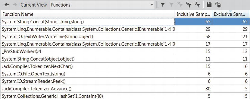
Figure 2-13 . Functions view, showing the functions with the most exclusive samples. The System.String.Concat function is responsible for twice as many samples as any other function
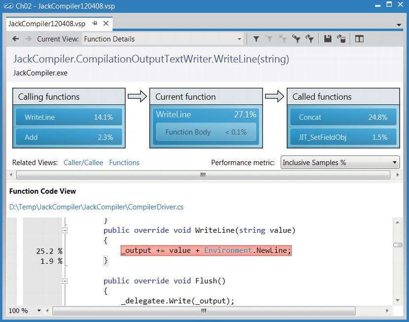
Figure 2-14 . Function Details view, showing the functions calling and called by the JackCompiler.CompilationOutputTextWriter.WriteLine function. In the function’s code, lines are highlighted according to the percent of inclusive samples they accumulated
![]() Caution It may appear that sampling is an accurate technique for measuring CPU utilization. You might hear claims that go as far as “if this method had 65% of the exclusive samples, then it ran for 65% of the time”. Because of the statistical nature of sampling, such reasoning is treacherous and should be avoided in practical use. There are several factors that can contribute to the inaccuracy of sampling results: CPU clock rates can change hundreds of times every second during application execution, such that the correlation between the number of samples and actual CPU time is skewed; a method can be “missed” (underrepresented) if it happens not to be running when many samples were taken; a method can be overrepresented if it happens to be running when many samples were taken but finished quickly every time. To summarize, you should not consider the results of a sampling profiler to be an exact representation of where CPU time was spent, but rather a general outline of the application’s main CPU bottlenecks.
Caution It may appear that sampling is an accurate technique for measuring CPU utilization. You might hear claims that go as far as “if this method had 65% of the exclusive samples, then it ran for 65% of the time”. Because of the statistical nature of sampling, such reasoning is treacherous and should be avoided in practical use. There are several factors that can contribute to the inaccuracy of sampling results: CPU clock rates can change hundreds of times every second during application execution, such that the correlation between the number of samples and actual CPU time is skewed; a method can be “missed” (underrepresented) if it happens not to be running when many samples were taken; a method can be overrepresented if it happens to be running when many samples were taken but finished quickly every time. To summarize, you should not consider the results of a sampling profiler to be an exact representation of where CPU time was spent, but rather a general outline of the application’s main CPU bottlenecks.
The Visual Studio profiler offers more information in addition to the exclusive/inclusive sample tables for every method. We recommend that you explore the profiler’s windows yourself—the Call Tree view shows the hierarchy of calls in the application’s methods (compare to PerfMonitor’s top down analysis, Figure 2-8), the Lines view displays sampling information on the line level, and the Modules view groups methods by assembly, which can lead to quick conclusions about the general direction in which to look for a performance bottleneck.
Because all sampling intervals require the application thread that triggers them to be actively executing on the CPU, there is no way to obtain samples from application threads that are blocked while waiting for I/O or synchronization mechanisms. For CPU-bound applications, sampling is ideal; for I/O-bound applications, we’ll have to consider other approaches that rely on more intrusive profiling mechanisms.
Visual Studio Instrumentation Profiler
The Visual Studio profiler offers another mode of operation, called instrumentation profiling, which is tailored to measuring overall execution time and not just CPU time. This makes it suitable for profiling I/O-bound applications or applications that engage heavily in synchronization operations. In the instrumentation profiling mode, the profiler modifies the target binary and embeds within it measurement code that reports back to the profiler accurate timing and call count information for every instrumented method.
For example, consider the following method:
public static int InstrumentedMethod(int param) {
  List< int > evens = new List < int > ();
  for (int i = 0; i < param; ++i) {
   if (i % 2 == 0) {
   evens.Add(i);
   }
  }
  return evens.Count;
}
During instrumentation, the Visual Studio profiler modifies this method. Remember that instrumentation occurs at the binary level—your source code is not modified, but you can always inspect the instrumented binary with an IL disassembler, such as .NET Reflector. (In the interests of brevity, we slightly modified the resulting code to fit.)
public static int mmid = (int)
  Microsoft.VisualStudio.Instrumentation.g_fldMMID_2D71B909-C28E-4fd9-A0E7-ED05264B707A;
public static int InstrumentedMethod(int param) {
  _CAP_Enter_Function_Managed(mmid, 0x600000b, 0);
  _CAP_StartProfiling_Managed(mmid, 0x600000b, 0xa000018);
  _CAP_StopProfiling_Managed(mmid, 0x600000b, 0);
  List < int > evens = new List < int > ();
  for (int i = 0; i < param; i++) {
   if (i % 2 == 0) {
   _CAP_StartProfiling_Managed(mmid, 0x600000b, 0xa000019);
   evens.Add(i);
   _CAP_StopProfiling_Managed(mmid, 0x600000b, 0);
   }
  }
  _CAP_StartProfiling_Managed(mmid, 0x600000b, 0xa00001a);
  _CAP_StopProfiling_Managed(mmid, 0x600000b, 0);
  int count = evens.Count;
  _CAP_Exit_Function_Managed(mmid, 0x600000b, 0);
  return count;
}
The method calls beginning with _CAP are interop calls to the VSPerf110.dll module, which is referenced by the instrumented assembly. They are the ones responsible for measuring time and recording method call counts. Because instrumentation captures every method call made out of the instrumented code and captures method enter and exit locations, the information available at the end of an instrumentation run can be very accurate.
When the same application we’ve seen in Figures 2-12, 2-13, and 2-14 is run under instrumentation mode (you can follow along—it’s the JackCompiler.exe application), the profiler generates a report with a Summary view that contains similar information—the most expensive call path through the application, and the functions with most individual work. However, this time the information is not based on sample counts (which measure only execution on the CPU); it is based on precise timing information recorded by the instrumentation code. Figure 2-15 shows the Functions view, in which inclusive and exclusive times measured in milliseconds are available, along with the number of times the function has been called.
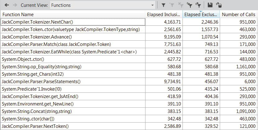
Figure 2-15 . The Functions view: System.String.Concat no longer appears to be the performance bottleneck, as our attention shifts to JackCompiler.Tokenizer.NextChar and JackCompiler.Token..ctor. The first method was called almost a million times
![]() Tip The sample application used to generate Figures 2-12 and 2-15 is not entirely CPU-bound; in fact, most of its time is spent blocking for I/O operations to complete. This explains the difference between sampling results, which point towards System.String.Concat as the CPU hog, and the instrumentation results, which point towards JackCompiler.Tokenizer.NextChar as the overall performance bottleneck.
Tip The sample application used to generate Figures 2-12 and 2-15 is not entirely CPU-bound; in fact, most of its time is spent blocking for I/O operations to complete. This explains the difference between sampling results, which point towards System.String.Concat as the CPU hog, and the instrumentation results, which point towards JackCompiler.Tokenizer.NextChar as the overall performance bottleneck.
Although instrumentation seems like the more accurate method, in practice you should try to keep to sampling if most of your application’s code is CPU-bound. Instrumentation limits flexibility because you must instrument the application’s code prior to launching it, and cannot attach the profiler to a process that was already running. Moreover, instrumentation has a non-negligible overhead—it increases code size significantly and places a runtime overhead as probes are collected whenever the program enters or exits a method. (Some instrumentation profilers offer a line-instrumentation mode, where each line is surrounded by instrumentation probes; these are even slower!)
As always, the biggest risk is placing too much trust in the results of an instrumentation profiler. It is reasonable to assume that the number of calls to a particular method does not change because the application is running with instrumentation, but the time information collected may still be significantly skewed because of the profiler’s overhead, despite any attempts by the profiler to offset the instrumentation costs from the final results. When used carefully, sampling and instrumentation can offer great insight into where the application is spending time, especially when you compare multiple reports and take note whether your optimizations are yielding fruit.
Advanced Uses of Time Profilers
Time profilers have additional tricks up their sleeves that we haven’t examined in the previous sections. This chapter is too short to discuss them in considerable detail, but they are worth pointing out to make sure you don’t miss them in the comforts of Visual Studio’s wizards.
As we saw in the Visual Studio Sampling Profiler section, the sampling profiler can collect samples from several types of events, including cache misses and page faults. In Chapters 5 and 6 we will see several examples of applications that can benefit greatly from improving their memory access characteristics, primarily around minimizing cache misses. The profiler will prove valuable in analyzing the number of cache misses and page faults exhibited by these applications and their precise locations in code. (When using instrumentation profiling, you can still collect CPU counters such as cache misses, instructions retired, and mispredicted branches. To do so, open the performance session properties from the Performance Explorer pane, and navigate to the CPU Counters tab. The collected information will be available as additional columns in the report’s Functions view.)
The sampling profiling mode is generally more flexible than instrumentation. For example, you can use the Performance Explorer pane to attach the profiler (in sampling mode) to a process that is already running.
Collecting Additional Data While Profiling
In all profiling modes, you can use the Performance Explorer pane to pause and resume the data collection when the profiler is active, and to generate markers that will be visible in the final profiler report to discern more easily various parts of the application’s execution. These markers will be visible in the report’s Marks view.
![]() Tip The Visual Studio profiler even has an API that applications can use to pause and resume profiling from code. This can be used to avoid collecting data from uninteresting parts of the application, and to decrease the size of the profiler’s data files. For more information about the profiler APIs, consult the MSDN documentation at http://msdn.microsoft.com/en-us/library/bb514149(v=vs.110).aspx.
Tip The Visual Studio profiler even has an API that applications can use to pause and resume profiling from code. This can be used to avoid collecting data from uninteresting parts of the application, and to decrease the size of the profiler’s data files. For more information about the profiler APIs, consult the MSDN documentation at http://msdn.microsoft.com/en-us/library/bb514149(v=vs.110).aspx.
The profiler can also collect Windows performance counters and ETW events (discussed earlier in this chapter) during a normal profiling run. To enable these, open the performance session properties from Performance Explorer, and navigate to the Windows Events and Windows Counters tabs. ETW trace data can only be viewed from the command line, by using the VSPerfReport /summary:ETW command line switch, whereas performance counter data will appear in the report’s Marks view in Visual Studio.
Finally, if Visual Studio takes a long time analyzing a report with lots of additional data, you can make sure it was a one-time performance hit: after analysis completes, right-click the report in Performance Explorer and choose “Save Analyzed Report”. Serialized report files have the .vsps file extension and open instantaneously in Visual Studio.
Profiler Guidance
When opening a report in Visual Studio, you might notice a section called Profiler Guidance which contains numerous useful tips that detect common performance problems discussed elsewhere in the book, including:
- “Consider using StringBuilder for string concatenations”—a useful rule that may help lower the amount of garbage your application creates, thus reducing garbage collection times, discussed in Chapter 4.
- “Many of your objects are being collected in generation 2 garbage collection”—the mid-life crisis phenomenon for objects, also discussed in Chapter 4.
- “Override Equals and equality operator on value types”—an important optimization for commonly-used value types, discussed in Chapter 3.
- “You may be using Reflection excessively. It is an expensive operation”—discussed in Chapter 10.
Advanced Profiling Customization
Collecting performance information from production environments may prove difficult if you have to install massive tools such as Visual Studio. Fortunately, the Visual Studio profiler can be installed and run in production environments without the entire Visual Studio suite. You can find the profiler setup files on the Visual Studio installation media, in the Standalone Profiler directory (there are separate versions for 32- and 64-bit systems). After installing the profiler, follow the instructions at http://msdn.microsoft.com/en-us/library/ms182401(v=vs.110).aspx to launch your application under the profiler or attach to an existing process using the VSPerfCmd.exe tool. When done, the profiler will generate a .vsp file that you can open on another machine with Visual Studio, or use the VSPerfReport.exe tool to generate XML or CSV reports that you can review on the production machine without resorting to Visual Studio.
For instrumentation profiling, many customization options are available from the command line, using the VSInstr.exe tool. Specifically, you can use the START, SUSPEND, INCLUDE, and EXCLUDE options to start and suspend profiling in a specific function, and to include/exclude functions from instrumentation based on a pattern in their name. More information about VSInstr.exe is available on the MSDN at http://msdn.microsoft.com/en-us/library/ms182402.aspx.
Some time profilers offer a remote profiling mode, which allows the main profiler UI to run on one machine and the profiling session to take place on another machine without copying the performance report manually. For example, the JetBrains dotTrace profiler supports this mode of operation through a small remote agent that runs on the remote machine and communicates with the main profiler UI. This is a good alternative to installing the entire profiler suite on the production machines.
![]() Note In Chapter 6 we will leverage the GPU for super-parallel computation, leading to considerable (more than 100×!) speedups. Standard time profilers are useless when the performance problem is in the code that runs on the GPU. There are some tools that can profile and diagnose performance problems in GPU code, including Visual Studio 2012. This subject is outside the scope of this chapter, but if you’re using the GPU for graphics or plain computation you should research the tools applicable to your GPU programming framework (such as C++ AMP, CUDA, or OpenCL).
Note In Chapter 6 we will leverage the GPU for super-parallel computation, leading to considerable (more than 100×!) speedups. Standard time profilers are useless when the performance problem is in the code that runs on the GPU. There are some tools that can profile and diagnose performance problems in GPU code, including Visual Studio 2012. This subject is outside the scope of this chapter, but if you’re using the GPU for graphics or plain computation you should research the tools applicable to your GPU programming framework (such as C++ AMP, CUDA, or OpenCL).
In this section, we have seen in sufficient detail how to analyze the application’s execution time (overall or CPU only) with the Visual Studio profiler. Memory management is another important aspect of managed application performance. Through the next two sections, we will discuss allocation profilers and memory profilers, which can pinpoint memory-related performance bottlenecks in your applications.
Allocation profilers detect memory allocations performed by an application and can report which methods allocated most memory, which types were allocated by each method, and similar memory-related statistics. Memory-intensive applications can often spend a significant amount of time in the garbage collector, reclaiming memory that was previously allocated. As we will see in Chapter 4, the CLR makes it very easy and inexpensive to allocate memory, but recovering it can be quite costly. Therefore, a group of small methods that allocate lots of memory may not take a considerable amount of CPU time to run—and will be almost invisible in a time profiler’s report—but will cause a slowdown by inflicting garbage collections at nondeterministic points in the application’s execution. We have seen production applications that were careless with memory allocations, and were able to improve their performance—sometimes by a factor of 10—by tuning their allocations and memory management.
We’ll use two tools for profiling memory allocations—the ubiquitous Visual Studio profiler, which offers an allocation profiling mode, and CLR Profiler, which is a free stand-alone tool. Unfortunately, both tools often introduce a significant performance hit to memory-intensive applications, because every memory allocation must go through the profiler for record-keeping. Nonetheless, the results can be so valuable that even a 100× slowdown is worth the wait.
Visual Studio Allocation Profiler
The Visual Studio profiler can collect allocation information and object lifetime data (which objects were reclaimed by the garbage collector) in the sampling and instrumentation modes. When using this feature with sampling, the profiler collects allocation data from the entire process; with instrumentation, the profiler collects only data from instrumented modules.
You can follow along by running the Visual Studio profiler on the JackCompiler.exe sample application from this chapter’s source code folder. Make sure to select “.NET memory allocation” in the Visual Studio Performance Wizard. At the end of the profiling process, the Summary view shows the functions allocating most memory and the types with most memory allocated (see Figure 2-16). The Functions view in the report contains for each method the number of objects and number of bytes that method allocated (inclusive and exclusive metrics are provided, as usual) and the Function Details view can provide caller and callee information, as well as color-highlighted source code with allocation information in the margins (see Figure 2-17). More interesting information is in the Allocation view, which shows which call trees are responsible for allocating specific types (see Figure 2-18).
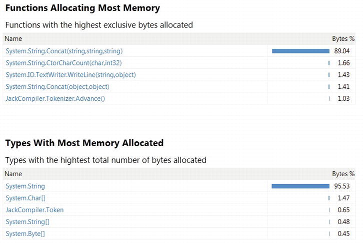
Figure 2-16 . Summary view from allocation profiling results
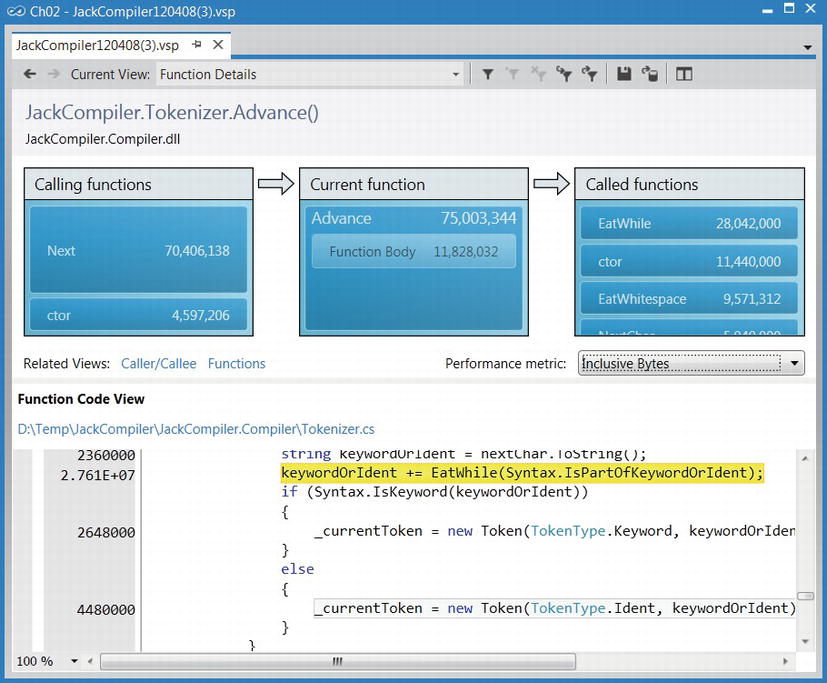
Figure 2-17 . Function Details view for the JackCompiler.Tokenizer.Advance function, showing callers, callees, and the function’s source with allocation counts in the margin
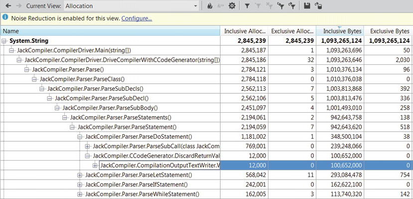
Figure 2-18 . Allocation view, showing the call tree responsible for allocating System.String objects
In Chapter 4 we will learn to appreciate the importance of quickly discarding temporary objects, and discuss a critical performance-related phenomenon called mid-life crisis, which occurs when temporary objects survive too many garbage collections. To identify this phenomenon in an application, the Object Lifetime view in the profiler’s report can indicate in which generation objects are being reclaimed, which helps understand whether they survive too many garbage collections. In Figure 2-19 you can see that all of the strings allocated by the application (more than 1GB of objects!) have been reclaimed in generation 0, which means they didn’t survive even a single garbage collection.
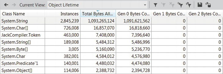
Figure 2-19 . The Object Lifetime view helps identify temporary objects that survive many garbage collections. In this view, all objects were reclaimed in generation 0, which is the cheapest kind of garbage collection available. (See Chapter 4 for more details.)
Although the allocation reports generated by the Visual Studio profiler are quite powerful, they are somewhat lacking in visualization. For example, tracing through allocation call stacks for a specific type is quite time-consuming if it is allocated in many places (as strings and byte arrays always are). CLR Profiler offers several visualization features, which make it a valuable alternative to Visual Studio.
CLR Profiler is a stand-alone profiling tool that requires no installation and takes less than 1MB of disk space. You can download it from http://www.microsoft.com/download/en/details.aspx?id=16273. As a bonus, it ships with complete sources, making for an interesting read if you’re considering developing a custom tool using the CLR Profiling API. It can attach to a running process (as of CLR 4.0) or launch an executable, and record all memory allocations and garbage collection events.
While running CLR Profiler is extremely easy—run the profiler, click Start Application, select your application, and wait for the report to appear—the richness of the report’s information can be somewhat overwhelming. We will go over some of the report’s views; the complete guide to CLR Profiler is the CLRProfiler.doc document, which is part of the download package. As always, you can follow along by running CLR Profiler on the JackCompiler.exe sample application.
Figure 2-20 shows the main view, generated after the profiled application terminates. It contains basic statistics concerning memory allocations and garbage collections. There are several common directions to take from here. We could focus on investigation memory allocation sources to understand where the application creates most of its objects (this is similar to the Visual Studio profiler’s Allocations view). We could focus on the garbage collections to understand which objects are being reclaimed. Finally, we could inspect visually the heap’s contents to understand its general structure.
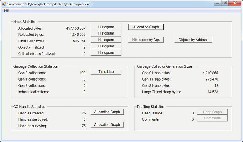
Figure 2-20 . CLR Profiler’s main report view, showing allocation and garbage collection statistics
The Histogram buttons next to “Allocated bytes” and “Final heap bytes” in Figure 2-20 lead to a graph of object types grouped into bins according to their size. These histograms can be used to identify large and small objects, as well as the gist of which types the program is allocating most frequently. Figure 2-21 shows the histogram for all the objects allocated by our sample application during its run.
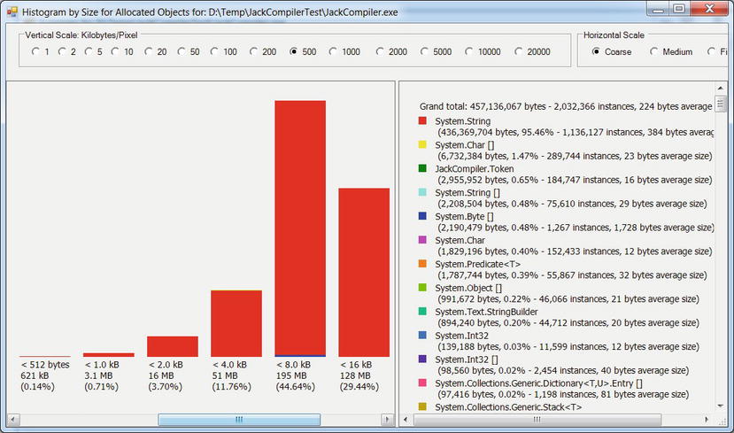
Figure 2-21 . All objects allocated by the profiled application. Each bin represents objects of a particular size. The legend on the left contains the total number of bytes and instances allocated from each type
The Allocation Graph button in Figure 2-20 opens a view that shows the allocating call stacks for all the objects in the application in a grouped graph that makes it easy to navigate from the methods allocating most memory to individual types and see which methods allocated their instances. Figure 2-22 shows a small part of the allocation graph, starting from the Parser.ParseStatement method that allocated (inclusively) 372MB of memory, and showing the various methods it called in turn. (Additionally, the rest of CLR Profiler’s views have a “Show who’s allocated” context menu item, which opens an allocation graph for a subset of the application’s objects.)
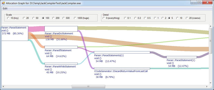
Figure 2-22 . Allocation graph for the profiled applications. Only methods are shown here; the actual types allocated are on the far right of the graph
The Histogram by Age button in Figure 2-20 displays a graph that groups objects from the final heap to bins according to their age. This enables quick identification of long-lived objects and temporaries, which is important for detecting mid-life crisis situations. (We will discuss these in depth in Chapter 4.)
The Objects by Address button in Figure 2-20 visualizes the final managed heap memory regions in layers; the lowest layers are the oldest ones (see Figure 2-23). Like an archaeological expedition, you can dig through the layers and see which objects comprise your application’s memory. This view is also useful for diagnosing internal fragmentation in the heap (e.g. due to pinning)—we will discuss these in more detail in Chapter 4.
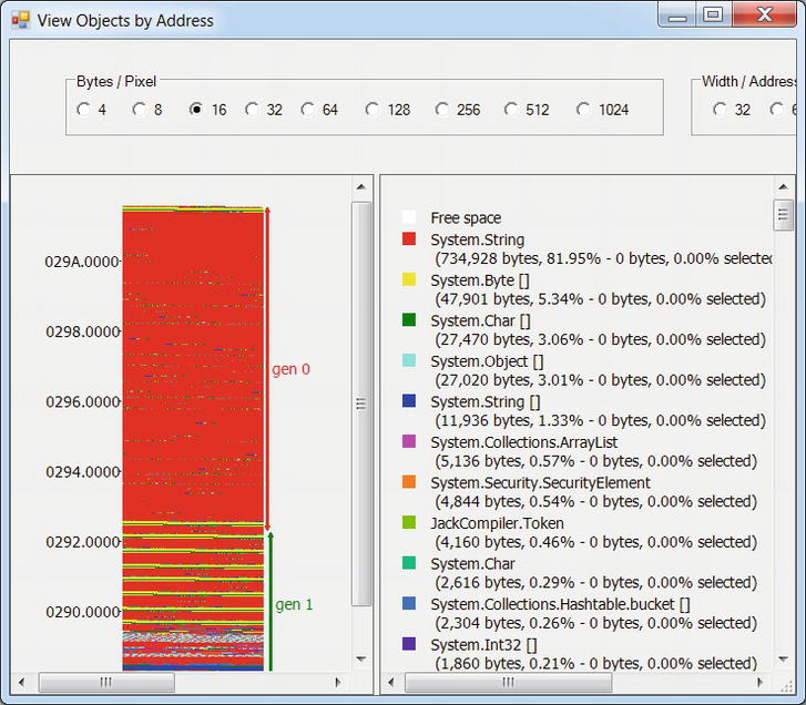
Figure 2-23 . Visual view of the application’s heap. The labels on the left axis are addresses; the “gen 0” and “gen 1” markers are subsections of the heap, discussed in Chapter 4
Finally, the Time Line button in the Garbage Collection Statistics section in Figure 2-20 leads to a visualization of individual garbage collections and their effect on the application’s heap (see Figure 2-24). This view can be used to identify which types of objects are being reclaimed, and how the heap is changing as garbage collections occur. It can also be instrumental in identifying memory leaks, where garbage collections do not reclaim enough memory because the application holds on to increasing amounts of objects.
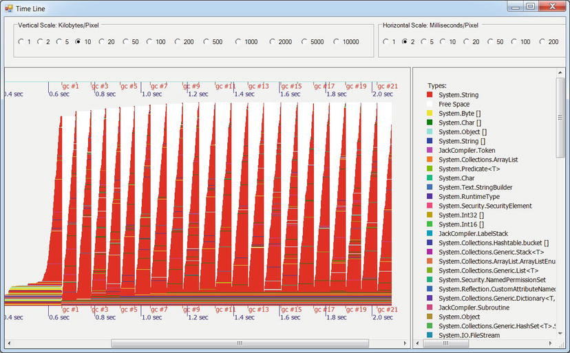
Figure 2-24 . Time line of an application’s garbage collections. The ticks on the bottom axis represent individual GC runs, and the area portrayed is the managed heap. As garbage collections occur, memory usage drops significantly and then rises steeply until the next collection occurs. Overall, memory usage (after GC) is constant, so this application is not exhibiting a memory leak
Allocation graphs and histograms are very useful tools, but sometimes it’s equally important to identify references between objects and not call stacks of methods. For example, when an application exhibits a managed memory leak, it can be very useful to crawl its heap, detect the largest object categories, and ascertain the object references that are preventing the GC from collecting these objects. While the profiled application is running, clicking the “Show Heap now” button generates a heap dump, which can be inspected later to categorize references between objects.
Figure 2-25 shows how three heap dumps are displayed simultaneously in the profiler’s report, showing a an increase in the number of byte[] objects retained by the f-reachable queue (discussed in Chapter 4), through Employee and Schedule object references. Figure 2-26 shows the result of selecting “Show New Objects” from the context menu to see only the objects allocated between the second and third heap dumps.
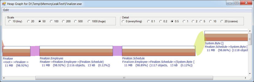
Figure 2-25 . Three heap dumps on top of one another, showing 11MB of byte[] instances being retained
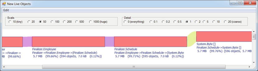
Figure 2-26 . The new objects allocated between the ultimate and penultimate heap dumps, showing that the source of the memory leak is clearly this reference chain from the f-reachable queue
You can use heap dumps in CLR Profiler to diagnose memory leaks in your applications, but the visualization tools are lacking. The commercial tools we discuss next offer richer capabilities, including automatic detectors for common memory leak sources, smart filters, and more sophisticated grouping. Because most of these tools don’t record information for each allocated object and don’t capture allocation call stacks, they introduce a lower overhead to the profiled application—a big advantage.
Memory Profilers
In this section we’ll discuss two commercial memory profilers that specialize in visualizing managed heaps and detecting memory leak sources. Because these tools are fairly complex, we will examine only a small subset of their features, and leave the rest to the reader to explore in the respective user guides.
RedGate’s ANTS Memory Profiler specializes in heap snapshot analysis. Below we detail the process for using ANTS Memory Profiler to diagnose a memory leak. If you would like to follow through with these steps as you read this section, download a free 14-day trial of ANTS Memory Profiler from http://www.red-gate.com/products/dotnet-development/ants-memory-profiler/ and use it to profile your own application. In the directions and screenshots below, we used ANTS Memory Profiler 7.3, which was the latest version available at the time of writing.
You can use the FileExplorer.exe application from this chapter’s source code folder to follow this demonstration—to make it leak memory, navigate the directory tree on the left to non-empty directories.
- Run the application from within the profiler. (Similarly to CLR Profiler, ANTS supports attaching to a running process, starting from CLR 4.0.)
- Use the Take Memory Snapshot button to capture an initial shapshot after the application has finished initializing. This snapshot is the baseline for subsequent performance investigations.
- As the memory leak accumulates, take additional heap snapshots.
- After the application terminates, compare snapshots (the baseline snapshot to the last snapshot, or intermediate snapshots among themselves) to understand which types of objects are growing in memory.
- Focus on specific types using the Instance Categorizer to understand what kinds of references are retaining objects of the suspected types. (At this phase you are inspecting references between types—instances of type A referencing instances of type B will be grouped by type, as if A is referencing B.)
- Explore individual instances of the suspected types using the Instance List. Identify several representative instances and use the Instance Retention Graph to determine why they are retained in memory. (At this phase you are inspecting references between individual objects, and can see why specific objects are not reclaimed by the GC.)
- Return to the application’s source code and modify it such that the leaking objects are no longer referenced by the problematic chain.
At the end of the analysis process, you should have a good grasp of why the heaviest objects in your application are not being reclaimed by the GC. There are many causes of memory leaks, and the real art is to quickly discern from the haystack that is a million-object heap the interesting representative objects and types that will lead to the major leak sources.
Figure 2-27 shows the comparison view between two snapshots. The memory leak (in bytes) consists primarily of string objects. Focusing on the string type in the Instance Categorizer (in Figure 2-28) leads to the conclusion that there is an event that retains FileInformation instances in memory, and they in turn hold references to byte[] objects. Drilling down to inspect specific instances using the Instance Retention Graph (see Figure 2-29) points to the FileInformation.FileInformationNeedsRefresh static event as the source of the memory leak.
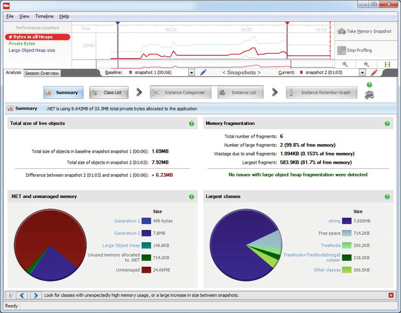
Figure 2-27 . Comparison between two heap snapshots. The total difference between them is +6.23MB, and the largest type currently held in memory is System.String
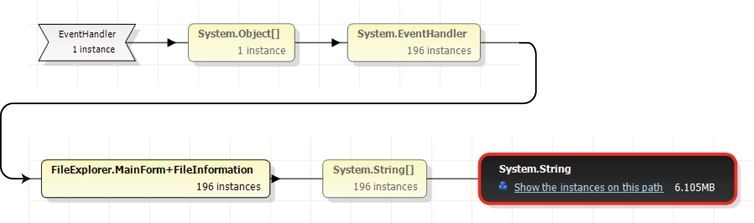
Figure 2-28 . The strings are retained by arrays of strings, which are retained by FileInformation instances, which are in turn retained by an event (through System.EventHandler delegates)
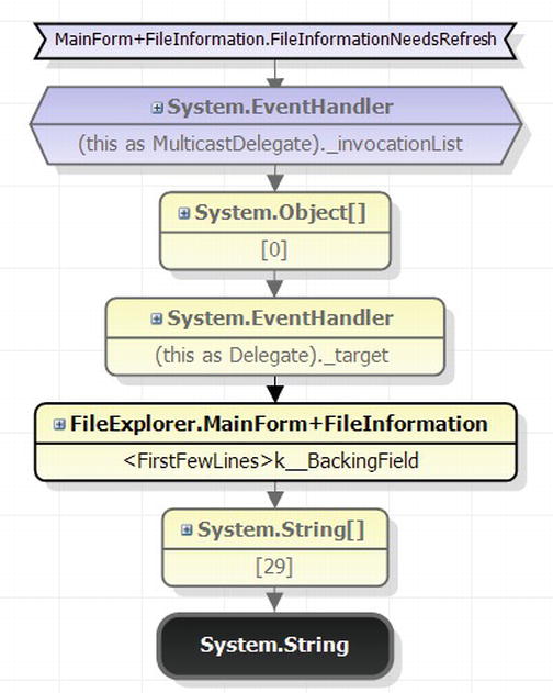
Figure 2-29 . The individual string we chose to examine is element 29 in an array of strings, held by the < FirstFewLines > k__BackingField field of a FileInformation object. Following the references points to the FileInformation.FileInformationNeedsRefresh static event
The SciTech .NET Memory Profiler is another commercial tool focused on memory leak diagnostics. Whereas the general analysis flow is quite similar to ANTS Memory Profiler, this profiler can open dump files, which means you don’t have to run it alongside the application and can use a crash dump generated when the CLR runs out of memory. This can be of paramount importance for diagnosing memory leaks post mortem, after the problem has already occurred in the production environment. You can download a 10-day evaluation version from http://memprofiler.com/download.aspx. In the directions and screenshots below, we used .NET Memory Profiler 4.0, which was the latest version available at the time of writing.
![]() Note CLR Profiler can’t open dump files directly, but there is an SOS.DLL command called !TraverseHeap that can generate a .log file in CLR Profiler’s format. We discuss more examples of SOS.DLL commands in Chapters 3 and 4. In the meantime, Sasha Goldshtein’s blog post at http://blog.sashag.net/archive/2008/04/08/next-generation-production-debugging-demo-2-and-demo-3.aspx provides an example of how to use SOS.DLL and CLR Profiler together.
Note CLR Profiler can’t open dump files directly, but there is an SOS.DLL command called !TraverseHeap that can generate a .log file in CLR Profiler’s format. We discuss more examples of SOS.DLL commands in Chapters 3 and 4. In the meantime, Sasha Goldshtein’s blog post at http://blog.sashag.net/archive/2008/04/08/next-generation-production-debugging-demo-2-and-demo-3.aspx provides an example of how to use SOS.DLL and CLR Profiler together.
To open a memory dump in .NET Memory Profiler, choose the File ![]() Import memory dump menu item and direct the profiler to the dump file. If you have several dump files, you can import them all into the analysis session and compare them as heap snapshots. The import process can be rather lengthy, especially where large heaps are involved; for faster analysis sessions, SciTech offers a separate tool, NmpCore.exe, which can be used to capture a heap session in a production environment instead of relying on a dump file.
Import memory dump menu item and direct the profiler to the dump file. If you have several dump files, you can import them all into the analysis session and compare them as heap snapshots. The import process can be rather lengthy, especially where large heaps are involved; for faster analysis sessions, SciTech offers a separate tool, NmpCore.exe, which can be used to capture a heap session in a production environment instead of relying on a dump file.
Figure 2-30 shows the results of comparing two memory dumps in .NET Memory Profiler. It has immediately discovered suspicious objects held in memory directly by event handlers, and directs the analysis towards the FileInformation objects.
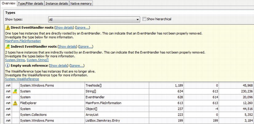
Figure 2-30 . Initial analysis of two memory snapshots. The first column lists the number of live instances, whereas the third columns lists the number of bytes occupied by them. The main memory hog—string objects—are not visible because of the tooltip
Focusing on the FileInformation objects illustrates that there is a single root path from the FileInformation.FileInformationNeedsRefresh event handler to the selected FileInformation instances (see Figure 2-31) and a visualization of individual instances confirms the same reference chain we have seen previously with ANTS Memory Profiler.
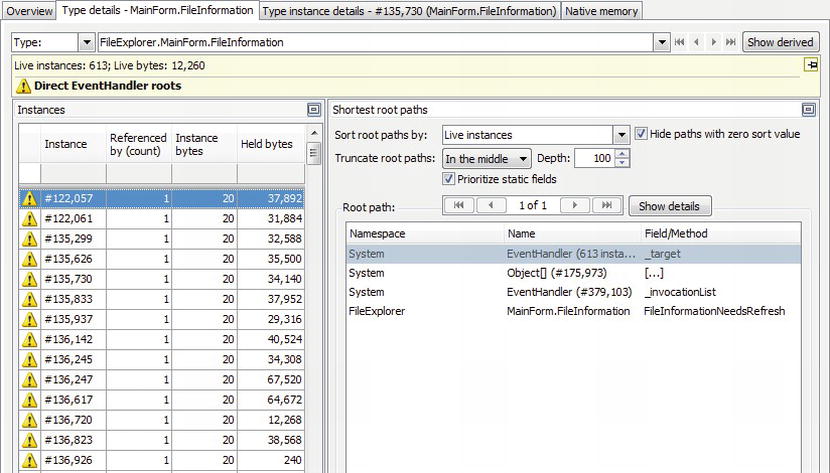
Figure 2-31 . FileInformation instances. The “Held bytes” column lists the amount of memory retained by each instance (its subtree in the object graph). On the right the shortest root path for the instance is shown
We will not repeat here the instructions for using the rest of .NET Memory Profiler’s functionality—you can find excellent tutorials on SciTech’s website, http://memprofiler.com/OnlineDocs/. This tool concludes our survey of memory leak detection tools and techniques, which begun with CLR Profiler’s heap dumps.
Other Profilers
In this chapter, we chose to focus mostly on CPU, time, and memory profilers, because these are the metrics on which most performance investigations focus. There are several other performance metrics that have dedicated measurement tools; in this section we will briefly mention some of them.
Database and Data Access Profilers
Many managed applications are built around a database and spend a significant portion of their time waiting for it to return query results or complete bulk updates. Database access can be profiled at two locations: from the application’s side, which is the realm of data access profilers, and from the database’s side, best left to database profilers.
Database profilers often require vendor-specific expertise, and are typically used by database administrators in their performance investigations and routine work. We will not consider database profilers here; you can read more about the SQL Server Profiler, which is a very powerful database profiling tool for Microsoft SQL Server, at http://msdn.microsoft.com/en-us/library/ms181091.aspx.
Data access profilers, on the other hand, are well within the domain of application developers. These tools instrument the application’s data access layer (DAL) and typically report the following:
- The database queries executed by the application’s DAL, and the precise stack trace that initiated each operation.
- The list of application methods that initiated a database operation, and the list of queries that each method has run.
- Alerts for inefficient database accesses, such as performing queries with an unbounded result set, retrieving all table columns while using only some of them, issuing a query with too many joins, or making one query for an entity with N associated entities and then another query for each associated entity (also known as the “SELECT N + 1” problem).
There are several commercial tools that can profile application data access patterns. Some of them work only with specific database products (such as Microsoft SQL Server), while others work with only a specific data access framework (such as Entity Framework or NHibernate). Below are a few examples:
- RedGate ANTS Performance Profiler can profile application queries to a Microsoft SQL Server database.
- Visual Studio “Tier Interactions” profiling feature can profile any synchronous data access operation from ADO.NET—unfortunately, it does not report call stacks for database operations.
- The Hibernating Rhinos family of profilers (LINQ to SQL Profiler, Entity Framework Profiler, and NHibernate Profiler) can profile all operations performed by a specific data access framework.
We will not discuss these profilers in more detail here, but if you are concerned about the performance of your data access layer, you should consider running them alongside with a time or memory profiler in your performance investigations.
The rising popularity of parallel programming warrants specialized profilers for highly concurrent software that uses multiple threads to run on multiple processors. In Chapter 6 we will examine several scenarios in which easily ripe performance gains are available from parallelization—and these performance gains are best realized with an accurate measurement tool.
The Visual Studio profiler in its Concurrency and Concurrency Visualizer modes uses ETW to monitor the performance of concurrent applications and report several useful views that facilitate detecting scalability and performance bottlenecks specific to highly concurrent software. It has two modes of operation demonstrated below.
Concurrency mode (or resource contention profiling) detects resources, such as managed locks, on which application threads are waiting. One part of the report focuses on the resources themselves, and the threads that were blocked waiting for them—this helps find and eliminate scalability bottlenecks (see Figure 2-32). Another part of the report displays contention information for a specific thread, i.e. the various synchronization mechanisms for which the thread had to wait—this helps reduce obstacles in a specific thread’s execution. To launch the profiler in this mode of operation, use the Performance Explorer pane or Analyze ![]() Launch Performance Wizard menu item and select the Concurrency mode.
Launch Performance Wizard menu item and select the Concurrency mode.
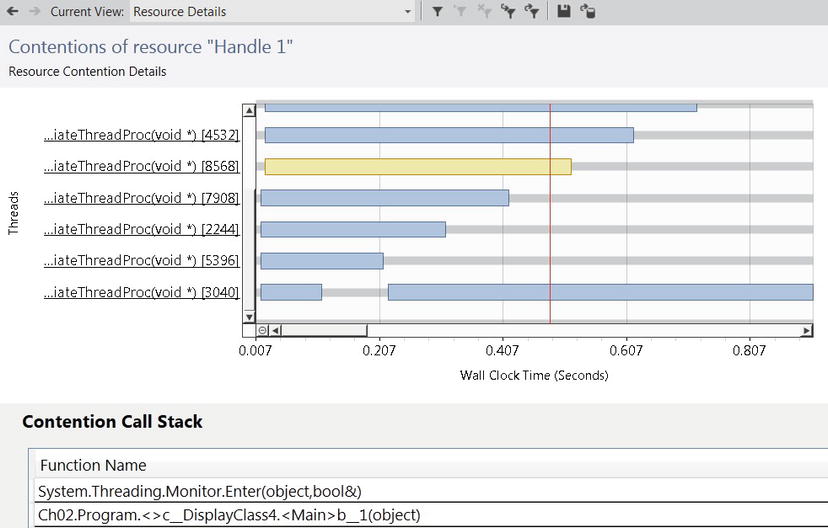
Figure 2-32 . Contention for a specific resource—there are several threads waiting at once to acquire the resource. When a thread is selected, its blocking call stack is listed on the bottom
Concurrency Visualizer mode (or multithreaded execution visualization) displays a graph with the execution details of all application threads, color-coded according to their current state. Every thread state transition—blocking for I/O, waiting for a synchronization mechanism, running—is recorded, along with its call stack and unblocking call stack when applicable (see Figure 2-33). These reports are very helpful for understanding the role of application threads, and detecting poor performance patterns such as oversubscription, undersubscription, starvation, and excessive synchronization. There’s also built-in support in the graph for Task Parallel Library mechanisms such as parallel loops, and CLR synchronization mechanisms. To launch the profiler in this mode of operation, use the Analyze ![]() Concurrency Visualizer sub-menu.
Concurrency Visualizer sub-menu.
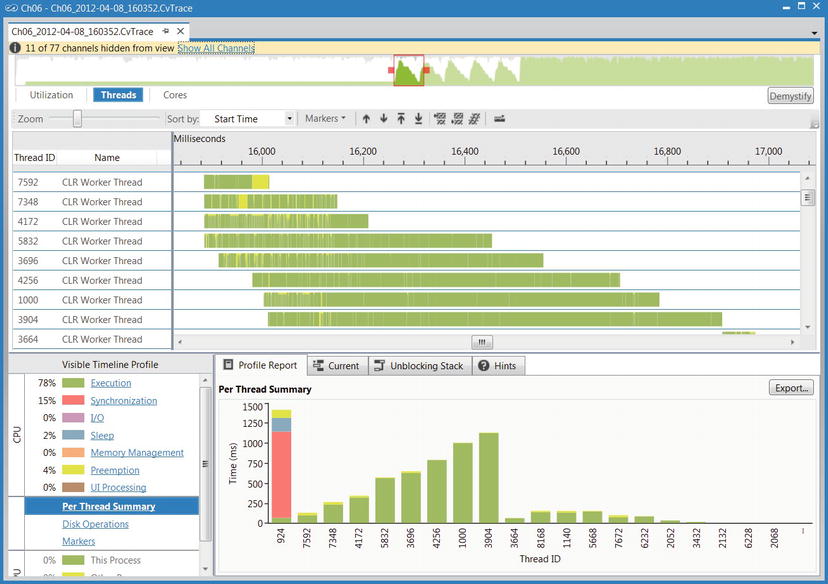
Figure 2-33 . Visualization of several application threads (listed on the left) and their execution. From the visualization and the histogram on the bottom it is evident that work was not distributed evenly between the different threads
![]() Note MSDN features a collection of anti-patterns for multithreaded applications based on Concurrency Visualizer graphs, including lock convoy, uneven workload distribution, oversubscription, and others—you can find these anti-patterns online at http://msdn.microsoft.com/en-us/library/ee329530(v=vs.110).aspx. When you run your own measurements, you’ll be able to identify similar problems by visually comparing the reports.
Note MSDN features a collection of anti-patterns for multithreaded applications based on Concurrency Visualizer graphs, including lock convoy, uneven workload distribution, oversubscription, and others—you can find these anti-patterns online at http://msdn.microsoft.com/en-us/library/ee329530(v=vs.110).aspx. When you run your own measurements, you’ll be able to identify similar problems by visually comparing the reports.
Concurrency profiling and visualization are highly useful tools, and we will meet them again in subsequent chapters. They serve as another great evidence of ETW’s great influence—this omnipresent high-performance monitoring framework is used across managed and native profiling tools.
The last performance metric category we study in this chapter is I/O operations. ETW events can be used to obtain counts and details for physical disk access, page faults, network packets, and other types of I/O, but we haven’t seen any specialized treatment for I/O operations.
Sysinternals Process Monitor is a free tool that collects file system, registry, and network activity (see Figure 2-34). You can download the entire suite of Sysinternals tools, or just the latest version of Process Monitor, from the TechNet website at http://technet.microsoft.com/en-us/sysinternals/bb896645. By applying its rich filtering capabilities, system administrators and performance investigators use Process Monitor to diagnose I/O-related errors (such as missing files or insufficient permissions) as well as performance problems (such as remote file system accesses or excessive paging).

Figure 2-34 . Process Monitor showing several types of events in the main view and the call stack for a specific event in the dialog window. Frames 19 and lower are managed frames
Process Monitor offers a complete user-mode and kernel-mode stack trace for each event it captures, making it ideal to understand where excessive or erroneous I/O operations are originating in the application’s source code. Unfortunately, at the time of writing Process Monitor cannot decode managed call stacks—but it can at least point in the general direction of the application that performed the I/O operation.
Through the course of this chapter we used automatic tools that measure application performance from various aspects—execution time, CPU time, memory allocation, and even I/O operations. The variety of measurement techniques is overwhelming, which is one of the reasons why developers often like to perform manual benchmarks of their application’s performance. Before concluding this chapter, we discuss microbenchmarking and some of its potential pitfalls.
Some performance problems and questions can only be resolved by manual measurement. You might be settling a bet about whether it’s worthwhile to use a StringBuilder, measuring the performance of a third party library, optimizing a delicate algorithm by unrolling inner loops, or helping the JIT place commonly used data into registers by trial and error—and you might not be willing to use a profiler to do the performance measurements for you because the profiler is either too slow, too expensive, or too cumbersome. Though often perilous, microbenchmarking is still very popular. If you do it, we want to make sure that you do it right.
We start with an example of a poorly designed microbenchmark and improve it until the results it provides are meaningful and correlate well with factual knowledge about the problem domain. The purpose is to determine which is faster—using the is keyword and then casting to the desired type, or using the as keyword and relying on the result.
//Test class
class Employee {
  public void Work() {}
}
//Fragment 1 – casting safely and then checking for null
static void Fragment1(object obj) {
  Employee emp = obj as Employee;
  if (emp ! = null) {
   emp.Work();
  }
}
//Fragment 2 – first checking the type and then casting
static void Fragment2(object obj) {
  if (obj is Employee) {
   Employee emp = obj as Employee;
   emp.Work();
  }
}
A rudimentary benchmarking framework might go along the following lines:
static void Main() {
  object obj = new Employee();
  Stopwatch sw = Stopwatch.StartNew();
  for (int i = 0; i < 500; i++) {
   Fragment1(obj);
  }
  Console.WriteLine(sw.ElapsedTicks);
  sw = Stopwatch.StartNew();
  for (int i = 0; i < 500; i++) {
   Fragment2(obj);
  }
  Console.WriteLine(sw.ElapsedTicks);
}
This is not a convincing microbenchmark, although the results are fairly reproducible. More often than not, the output is 4 ticks for the first loop and 200-400 ticks for the second loop. This might lead to the conclusion that the first fragment is 50-100 times faster. However, there are significant errors in this measurement and the conclusion that stems from it:
- The loop runs only once and 500 iterations are not enough to reach any meaningful conclusions—it takes a negligible amount of time to run the whole benchmark, so it can be affected by many environmental factors.
- No effort was made to prevent optimization, so the JIT compiler may have inlined and discarded both measurement loops completely.
- The Fragment1 and Fragment2 methods measure not only the cost of the is and as keywords, but also the cost of a method invocation (to the Fragment N method itself!). It may be the cast that invoking the method is significantly more expensive than the rest of the work.
Improving upon these problems, the following microbenchmark more closely depicts the actual costs of both operations:
class Employee {
  //Prevent the JIT compiler from inlining this method (optimizing it away)
  [MethodImpl(MethodImplOptions.NoInlining)]
  public void Work() {}
}
static void Measure(object obj) {
  const int OUTER_ITERATIONS = 10;
  const int INNER_ITERATIONS = 100000000;
  //The outer loop is repeated many times to make sure we get reliable results
  for (int i = 0; i < OUTER_ITERATIONS; ++i) {
   Stopwatch sw = Stopwatch.StartNew();
   //The inner measurement loop is repeated many times to make sure we are measuring an
   //operation of significant duration
   for (int j = 0; j < INNER_ITERATIONS; ++j) {
   Employee emp = obj as Employee;
   if (emp ! = null)
   emp.Work();
   }
   Console.WriteLine("As - {0}ms", sw.ElapsedMilliseconds);
  }
  for (int i = 0; i < OUTER_ITERATIONS; ++i) {
   Stopwatch sw = Stopwatch.StartNew();
   for (int j = 0; j < INNER_ITERATIONS; ++j) {
   if (obj is Employee) {
   Employee emp = obj as Employee;
   emp.Work();
   }
   }
   Console.WriteLine("Is Then As - {0}ms", sw.ElapsedMilliseconds);
  }
}
The results on one of the author’s test machines (after discarding the first iteration) were around 410ms for the first loop and 440ms for the second loop, a reliable and reproducible performance difference, which might have you convinced that indeed, it’s more efficient to use just the as keyword for casts and checks.
However, the riddles aren’t over yet. If we add the virtual modifier to the Work method, the performance difference disappears completely, not even if we increase the number of iterations. This cannot be explained by the virtues or maladies of our microbenchmarking framework—it is a result from the problem domain. There is no way to understand this behavior without going to the assembly language level and inspecting the loop generated by the JIT compiler in both cases. First, before the virtual modifier:
; Disassembled loop body – the first loop
mov edx,ebx
mov ecx,163780h (MT: Employee)
call clr!JIT_IsInstanceOfClass (705ecfaa)
test eax,eax
je WRONG_TYPE
mov ecx,eax
call dword ptr ds:[163774h] (Employee.Work(), mdToken: 06000001)
WRONG_TYPE:
; Disassembled loop body – the second loop
mov edx,ebx
mov ecx,163780h (MT: Employee)
call clr!JIT_IsInstanceOfClass (705ecfaa)
test eax,eax
je WRONG_TYPE
mov ecx,ebx
cmp dword ptr [ecx],ecx
call dword ptr ds:[163774h] (Employee.Work(), mdToken: 06000001)
WRONG_TYPE:
In Chapter 3 we’ll discuss in great depth the instruction sequence emitted by the JIT compiler to call a non-virtual method and to call a virtual method. When calling a non-virtual method, the JIT compiler must emit an instruction that makes sure we are not making a method call on a null reference. The CMP instruction in the second loop serves that task. In the first loop, the JIT compiler is smart enough to optimize this check away, because immediately prior to the call, there is a null reference check on the result of the cast (if (emp ! = null) . . .). In the second loop, the JIT compiler’s optimization heuristics are not sufficient to optimize the check away (although it would have been just as safe), and this extra instruction is responsible for the extra 7-8% of performance overhead.
After adding the virtual modifier, however, the JIT compiler generates exactly the same code in both loop bodies:
; Disassembled loop body – both cases
mov edx,ebx
mov ecx,1A3794h (MT: Employee)
call clr!JIT_IsInstanceOfClass (6b24cfaa)
test eax,eax
je WRONG_TYPE
mov ecx,eax
mov eax,dword ptr [ecx]
mov eax,dword ptr [eax + 28h]
call dword ptr [eax + 10h]
WRONG_TYPE:
The reason is that when invoking a virtual method, there’s no need to perform a null reference check explicitly—it is inherent in the method dispatch sequence (as we will see in Chapter 3). When the loop bodies are identical, so are the timing results.
Microbenchmarking Guidelines
For successful microbenchmarks you have to make sure that what you decided to measure adheres to the following guidelines:
- Your test code’s environment is representative of the real environment for which it is being developed. For example, you should not run a method on in-memory data collections if it is designed to operate on database tables.
- Your test code’s inputs are representative of the real input for which it is being developed. For example, you should not measure how a sorting method fares on three-element lists if it is designed to operate on collections with several million elements.
- The supporting code used to set up the environment should be negligible compared to the actual test code you are measuring. If this is impossible, then the setup should happen once and the test code should be repeated many times.
- The test code should run for sufficiently long so as to be considerable and reliable in the face of hardware and software fluctuations. For example, if you are testing the overhead of a boxing operation on value types, a single boxing operation is likely to be too fast to produce significant results, and will require many iterations of the same test to become substantial.
- The test code should not be optimized away by the language compiler or the JIT compiler. This happens often in Release mode when trying to measure simple operations. (We will return to this point later.)
When you have ascertained that your test code is sufficiently robust and measures the precise effect that you intended to measure, you should invest some time in setting up the benchmarking environment:
- When the benchmark is running, no other processes should be allowed to run on the target system. Networking, file I/O, and other types of external activity should be minimized (for example, by disabling the network card and shutting down unnecessary services).
- Benchmarks that allocate many objects should be wary of garbage collection effects. It’s advisable to force a garbage collection before and after significant benchmark iterations to minimize their effects on each other.
- The hardware on the test system should be similar to the hardware to be used in the production environment. For example, benchmarks that involve intensive random disk seeks will run much faster on a solid state hard drive than a mechanical drive with a rotating head. (The same applies to graphics cards, specific processor features such as SIMD instructions, memory architecture, and other hardware traits.)
Finally, you should focus on the measurement itself. These are the things to keep in mind when designing benchmarking code:
- Discard the first measurement result—it is often influenced by the JIT compiler and other application startup costs. Moreover, during the first measurement data and instructions are unlikely to be in the processor’s cache. (There are some benchmarks that measure cache effects, and should not heed this advice.)
- Repeat measurements many times and use more than just the average—the standard deviation (which represents the variance of the results) and the fluctuations between consecutive measurements are interesting as well.
- Subtract the measurement loop’s overhead from the benchmarked code—this requires measuring the overhead of an empty loop, which isn’t trivial because the JIT compiler is likely to optimize away empty loops. (Writing the loop by hand in assembly language is one way of countering this risk.)
- Subtract the time measurement overhead from the timing results, and use the least expensive and most accurate time measurement approach available—this is usually System.Diagnostics.Stopwatch.
- Know the resolution, precision, and accuracy of your measurement mechanism—for example, Environment.TickCount’s precision is usually only 10-15ms, although its resolution appears to be 1ms.
![]() Note Resolution is the fineness of the measurement mechanism. If it reports results in integer multiples of 100ns, then its resolution is 100ns. However, its precision might be far less—for a physical time interval of 500ns it might report 2 × 100ns on one occasion and 7 × 100ns on another. We might be able to place an upper bound on the precision at 300ns, in this case. Finally, accuracy is the degree of correctness of the measurement mechanism. If it reliably and repeatedly reports a 5000ns physical time interval as 5400ns with a precision of 100ns, we might say its accuracy is +8% of the truth.
Note Resolution is the fineness of the measurement mechanism. If it reports results in integer multiples of 100ns, then its resolution is 100ns. However, its precision might be far less—for a physical time interval of 500ns it might report 2 × 100ns on one occasion and 7 × 100ns on another. We might be able to place an upper bound on the precision at 300ns, in this case. Finally, accuracy is the degree of correctness of the measurement mechanism. If it reliably and repeatedly reports a 5000ns physical time interval as 5400ns with a precision of 100ns, we might say its accuracy is +8% of the truth.
The unfortunate example in the beginning of this section should not dissuade you from ever writing your own microbenchmarks. However, you should mind the advice given here and design meaningful benchmarks whose results you can trust. The worst performance optimization is one that is based on incorrect measurements; unfortunately, manual benchmarking often leads into this trap.
Summary
Performance measurement is no simple task, and one of the reasons is the large variety of metrics and tools, and the effect of the tools on the measurement accuracy and the application’s behavior. We’ve seen a large number of tools in this chapter, and you might be feeling a little dizzy if asked to recite precisely which situations warrant the use of which tool. Table 2-3 summarizes the important characteristics of all the tools demonstrated in this chapter.
Table 2-3. The Performance Measurement Tools Used in This Chapter
Armed with these tools and general understanding of what performance metrics to expect from managed applications, we are ready now to dive into the internals of the CLR, and see what practical steps can be taken to improve the performance of managed applications.