
Appendix C: Inter-Symbol Interference Indexes Summation Rule
C.1 Cascade of Linear Filters
In this appendix, we will demonstrate the rule used in the design of transmission systems that, under opportune hypothesis, the ISI indexes relative to independent phenomena can be added.
We will consider regular pulses, that is, either finite duration pulses or pulses with exponentially decreasing tails, so that no convergence problem will arise in our calculation.
We will also assume in this appendix the following hypotheses:
The pulse p(t) at the filter chain input has a zero temporal mean that is
 . For example, it is a Gaussian pulse.
The linear filters of the chain have a pulse response a(t) with zero mean, that is,
 . This is true, for example, for Gaussian filters, which also have Gaussian pulse response, that is, with a good approximation for a large class of array waveguides (AWGs).
Let us imagine having a system constituted by the cascade of two linear filters. Let us assume that two linear operators  and ![]() represent the two filters that act on a pulse signal p(t) broadening it so that
represent the two filters that act on a pulse signal p(t) broadening it so that
![]()
the pulse width after the operators action is
![]()
and an analogous equation for τB. Changing variables into the integral and remembering the property of the pulse average to be zero, we have
![]()
where TA and TB are the widths of the pulse responses of the filters
Let us now apply the two filters together
![]()
the expression of the overall pulse widening is obtained by the following substitution in the integral:
![]()
The variable change has unitary Jacobian, and the integral becomes
![]()
from the integral, since all the pulses have zero mean, the following is derived:
![]()
C.2 Presence of One Nonlinear Operator with Fast Nonlinearity
In the cases that interest us, at least one of the involved filters is nonlinear, but with an instantaneous nonlinearity. It is a simplified way to represent the effect of the Kerr nonlinearity at the system output.
The filter ![]() is now composed of two parts: a linear part with memory and an instantaneous nonlinear part depending on the pulse power, so that
is now composed of two parts: a linear part with memory and an instantaneous nonlinear part depending on the pulse power, so that
![]()
As a first step, let us evaluate the pulse widening due to the transit through ![]() . This widening is given by
. This widening is given by
![]()
substituting z = t − ϑ in the integral and remembering that all pulses have zero mean, we obtain
![]()
The nonlinear broadening is complex to evaluate, depending on f( ); however, Equation C.10 is sufficient to reach our goal.
With the same procedure of the previous section, we can write the expression of the overall pulse widening as
![]()
C.3 Comments and Examples
As a comment, it is to be observed that the derivation we have done holds exactly only in very specific situations, where strict hypotheses like exponential tails and zero mean holds for all the pulses, both the signal and the pulse response of the filters.
Naturally, if these conditions are not fulfilled completely, the property will not hold exactly, but in a regime of small distortion, we can frequently use this fundamental rule.
As an example, let us consider a squared pulse 10 ps long with a rise time of 3 ps, as shown in Figure C.1. Let us filter the pulse with a first Gaussian filter of insufficient bandwidth, equal to 61 GHz instead of the required minimum of 100 GHz.
As a consequence of the filtering, the pulse spreads, as shown in Figure C.2, and assumes a standard deviation of 11.6 ps that is exactly the result of Equation C.3.
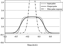
FIGURE C.1 Pulse at the input of the filter chain and after the first filter.
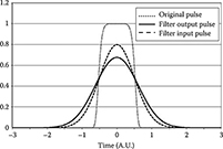
FIGURE C.2 Pulse at the input and at the output of the second filter.
Filtering again the pulse with another filter with an even smaller bandwidth (25.88 GHz in this case), the pulse broadens again reaching a width, as shown in Figure C.2. The final width is exactly what we have foreseen in Equation C.7.