
8 Convergent Network Management and Control Plane
8.1 Introduction
In Chapter 2 we have seen that the main target of major telecommunication carriers is to decrease the operational expenditure (OPEX) necessary to maintain and operate the network. In Chapter 3 we have seen that there are different implementations of IP over optical architecture, but it is a fact that the old architecture made by two independent networks, one for data and one for telephone, has almost disappeared everywhere.
With the convergence of transport over one architecture, independently on the service bundles offered by the carrier to different categories of customers, also the division of the network management in two completely different architectures becomes inefficient: central management for the physical transport (SDH/SONET and optical transport network [OTN]) and automatic control plane for the packet layer (IP and Ethernet) have to merge.
As a matter of fact, with the network technology evolution and the introduction of a great number of new services, static centralized management is demonstrated to be not suitable for the carriers needs.
It is true that TMN-based management had the merit of introducing a never before seen ability of controlling the network and of assuring performances and reliability, but with a traffic more and more dynamic, the great number of manual operations required by centralized network managers are a source of both costs and errors.
On the other hand, the packet layer is managed through an automatic control plane that, even if is sometimes poor in terms of reporting with respect to the carriers expectations, is very effective in decreasing costs and eliminating errors.
Thus, it is quite natural to envision a new control plane that is capable of automatically managing all the network layers in an integrated manner and is also sufficiently rich in functionalities so as to be at least comparable with traditional TMN.
Different initiatives are ongoing to create new control plane standards. In particular, ITU-T, the world standardization institute that is traditionally carrier-driven, has developed the automatic switched optical network (ASON) standard with the aim of providing a framework for the development of the convergent network control plane [1].
Also IETF, that is the facto the Internet standardization body and is traditionally vendordriven, has created the generalized-multiprotocol label switch (GMPLS) protocol suite, a complete control plane whose standardization is in some parts still ongoing, whose target is to generalize the ideas at the base of MPLS [32, 33, 34] to be able to manage not only packet-oriented networks, but also circuit-oriented networks like the WDM layer or the next generation SONET layer.
At a first glance, it could seem that ASON and GMPLS are two competing standards and that only one of them will prevail with time, but this is completely false. As a matter of fact, ASON is not a protocol suite, even if it gives a lot of recommendations about protocols, but it is more an architecture and a framework in which the protocols of the new control plane have to fit. Thus, it is well possible to fit GMPLS protocols in the ASON architecture, even if this is not completely free of work since the two standards were born independently.
The work of fitting GMPLS into the ASON architecture is ongoing in another industry standardization group: the Optical Internetworking Forum (OIF). The OIF is issuing a series of documents called implementation agreements (AI) [2] whose role is exactly to fit GMPLS into the ASON architecture pointing out where there are difficulties, corrections to be applied to existing GMPLS protocols or different interpretations of the ASON architecture.
Moreover, OIF is promoting a wide experimentation activity whose goal is to set up test beds for the new control plane that verify the functionalities of its parts. This is a very important activity since, if there is a sort of progressive experimental verification of the functions of the new control plane, they can be introduced gradually into the carrier networks, thereby distributing the costs over a long time and allowing the new procedures to be introduced progressively.
This chapter is divided into three parts: in the first we will analyze the ASON architecture, in the second we will review the GMPLS protocol suite, and in the third we will discuss how a multilayer network based on an integrated control plane can be designed and optimized.
8.2 ASON Architecture
8.2.1 ASON Network Model
Historically the control plane accompanies the packet-switched networks, which are not supposed to have a rich management plane as the transport networks. The first point to solve if a control plane is to be developed so to manage a whole network how will the control plane protocols and the network manager interact and how will they divide the functions.
As a matter of fact, several control plane functions are performed in traditional transport networks by the central network manager so that both control plane and network manager have to be redefined in a functional sense.
The ASON architecture states that the control plane is responsible for the actual resource and connection management within an automatically switched network (ASN). The control plane resides in a distributed network intelligence constituted by the optical connection controllers (OCCs); the OCC can run in separate workstations as the element managers but generally directly reside into the control unit of the equipments dedicated to switching at each network layer. The OCCs are interconnected via the interface called network to network interfaces (NNI) and run the control plane protocol suite having the following functions:
Network topology discovery (that is, resource discovery)
Address assignment to an equipment port when it is discovered and address advertisement to all the networks
Signaling (connections setup, management, and tear down)
Connections routing
Connection protection/restoration
Traffic engineering
Resource assignment (e.g., wavelength assignment in the WDM layer, time slot assignment in the SONET layer etc.)
The management plane is responsible for managing the control plane. Its responsibilities include the following:
Configuration management of the control plane resources
Definition of the administrative areas
Control plane policies definition
Few of the traditional network manager functionalities should also be maintained on the data plane entities:
Fault management
Performance management
Accounting and security management
The management plane is constituted by the central management unit, which runs the network manager, and the local management units, which run the element managers, and by the management network that connects all the entities of the management plane.
The central network management entity is connected to an OCC in control plane via the network management interface for ASON control plane (NMI-A) and to one of the switches via network management interface for the transport network (NMI-T).
Using these interfaces, the management plane can access to all the control plane entities via the control plane connectivity to perform control plane management and to all the data plane entities to perform reporting of data plane status and those functionalities that are responsibility of the management plane. The management structure of the ASON network is illustrated in Figure 8.1.
The network model on which the ASON standard is based is a multilayer model in which a single control plane coordinates the activity of all the layers. This vertical structure is reproduced in Figure 8.2, where there is evidence to show that all the layers define a specific physical or virtual connection, so that in its whole we can talk about a virtual connection–oriented network.
Connectionless layer can be clients of an ASON network, but cannot be managed by an ASON control plane. The ASON network is intrinsically a multilayer network and different network topologies can be defined at each layer. Let us refer just for an example to Figure 8.3 where a three layer network is represented.
At the base physical layer, there is the set of fiber cables represented by gray bold lines and the set of buildings that are the carrier points of presence in the area.
In all the buildings there is an optical cross connect (OXC), but not all the cables are equipped with WDM systems, quite a realistic situation due to the fact that cables are generally deployed with long-term plans that are completely independent of the network that will be realized on the cable infrastructure.
The WDM layer has probably different clients, one of that is an MPLS layer composed by a set of label-switched routers (LSRs). Not in all the nodes there is a LSR, but only in the nodes where such a machine is needed. As a consequence of this complex network architecture, three network topologies can be proposed: a physical network topology composed by cable ducts and buildings, a WDM virtual network topology composed by WDM systems and OXCs, and a MPLS virtual network topology composed by LSRs with the connectivity that is offered to them by the underlying transport layer

Figure 8.1 ASON standard layered model for the Automatic Switched Network management; standard interfaces between management and control plane (NMI-A) and between management and data plane (NMI-T) are shown.
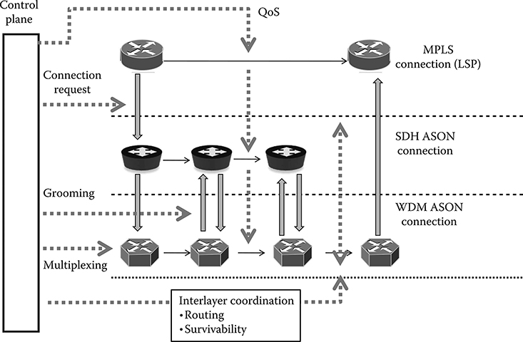
Figure 8.2 ASON Network model: a multilayer network in which a single control plane coordinates the activity of all the layers.

Figure 8.3 Scheme of a three layer network where the deployed equipment is shown in the physical topology plot (left side) and the virtual topologies at each layer are evidenced as graphs (right side).
The different topologies are shown as graphs in Figure 8.3.
The situation of this example can generally be replayed in all multilayer network architecture, identifying a specific topology (physical of virtual) at each layer of the network. Identifying the correct topology is very important since in a multilayer network managed by a single control plane, every routing element refers for its routing protocols to the topology that is specific to that layer.
Under a horizontal point of view, ASON is organized in administrative domains. The administrative domain is a part of the network that has its own autonomy, for example, the network belonging to a carrier in the framework on a national multicarrier network.
The concept of administrative domain is needed to allow the network to hide its own internal data to the overall network and to encapsulate all the internal addressing into a global network address so that they cannot be seen by other administrative domains. This hiding and encapsulating strategy has a twofold function: it is needed in order to allow carriers to hide data relative to their network to competitors even if roaming among different carriers have to be provided by the control plane, but it is also needed to reduce the dimension of the routing tables in the network routing elements. As a matter of fact, when the network is divided into administrative domains, every switching element stores the complete topology of its own domain and a metatopology relative to the connections with different domains. The partition of the ASON network is shown in Figure 8.4.

Figure 8.4 Domain partition of the ASON network model.
When a connection has to be set-up with a node in a different domain, the precise node address is encapsulated into the global domain address. The switch that has to set up the connection simply send a connection set-up protocol to the point of contact with the destination domain and it will be this node that is inside the domain of the connection end point to complete the connection setup establishing the path into the destination domain. This procedure is shown in Figure 8.5, where the logical working of encapsulation is shown.
Let us image that the address of every node is a couple of letters, so that node A of domain A has an address (A, A). Let us image that a connection has to be established from (A, A) to (B, B). The node (A, A) receives the instruction to open a connection to (*, B). The exact destination node address is hidden since it belongs to a different administrative domain whose topology is not known to node (A, A).
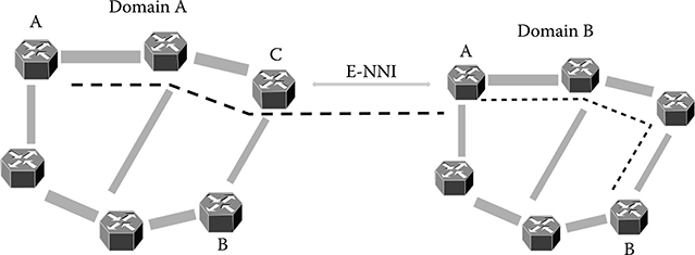
Figure 8.5 Example of inter-domain routing in an ASON network.
Node (A, A) has a routing table knowing that the external network to network (E-NNI) interface toward administrative domain B is between node (C, A) and (A, B) so node (A, A) sets up a link to node (C, A) that forwards the link through the interdomain interface to node (A, B).
Now Node (A, B) knows that a connection between node (*, A) is to set up with node (B, B) starting from the connection that was set up through the interdomain interface with domain A.
Node (A, B) knows exactly from the routing table the position within domain B of the node (B, B) and set up the second part of the connection, represented in the figure by the dotted line.
Besides the separation of information belonging to competitor carriers, in our example the administrative domain separation cause every node to store a topology made of six nodes: five in the same domain and one is a virtual node that is the connection with the other domain.
If all the information was shared among all the network nodes, every node should store a topology of 11 nodes. The concept of administrative domain is also a powerful instrument for the gradual introduction of the ASON architecture in carrier networks. As a matter of fact, an abrupt introduction of a new architecture in a big network like that of an incumbent carrier is not feasible. The new technology is in general introduced gradually in pace with CAPEX expenditure and market request.
Thus during the introduction of the ASON control plane, for a long time there will be parts of the carrier network that will include subsets of ASON features, possibly different subsets depending on the circumstances and on the kind of equipment the carrier has installed in that part of the network, and parts of the network that are not yet migrated.
The network has to work in this hybrid situation without any service disruption: this can be achieved by defining every area of the network where there is a different ASON-compatible technology as a different administrative domain, and interface these administrative domains with those parts of the network where ASON is not yet implemented by suitable interfaces.
Besides the administrative domains, the ASON standard defines another horizontal entity: the routing area. The routing area is generally a subpart of an administrative domain that has the characteristic to be represented by other routing areas like a single virtual node.
Thus, exactly like for the administrative domain, when a node external to the routing area wants to set up a connection with a node inside the routing area it sends the connection setup protocol to the virtual node representing all the routing area that physically corresponds to the point of contact of the destination routing area with the origination one.
Only when the connection setup protocol arrives at the gateway of the routing area it completes the connection setup inside the area. Differently from the administrative domain, routing areas are not insulated under an administrative point of view and the internal information is not completely hidden.
This is due to the different destination of the routing areas with respect to the adminis-trative domains: routing areas are used inside a big administrative domain to reduce the complexity of the address tables of the routing entities by introducing a routing hierarchy while the administrative domain serves mainly to divide parts of the network that have to be administrated independently either because they are owned by different carriers or because they are built on different technologies.
8.2.2 ASON Standard Interfaces
In correspondence to the structure of the network in administrative domains, the ASON standard defines a set of interfaces that are conceived for compatibility between different equipments and different particular implementations of the control plane.
As a matter of fact, it should be remembered that ASON is not a complete protocol suite, but more a reference architecture. Thus it is well possible that different vendors use different specific sets of protocols, all ASON-compatible.
In this case, naturally every different protocol suite will be confined to a different administrative domain and suitable interfaces will guarantee the cross-compatibility.
The first standard interface that is the optical user network interface (O-UNI). This is the interface connecting into the data plane the client equipment with a network equipment through an optical signal.
Somehow the O-UNI is a limited functionality interface, since it has also to shield the network from any improper client activity that could either interfere with the network working or try to detect information about the network that the carrier wants to hide to the customer.
The activity of the O-UNI is thus limited to resource discovery, signaling and, naturally, data exchange. In particular, the following protocols flow through the O-UNI:
Connection request and creation
Connection parameters change
Connection delete
Client identity change
Data transit
Just to do an example, it is through the O-UNI that the Ethernet switch belonging to a corporate network asks to the public network the creation of a virtual connection for a data center back-up operation.
In particular, the ASON-enabled Ethernet switch sends through the O-UNI a suitable signal to the multilayer node to which it is connected for specifying the request of a mission-critical data connection between two points of the network. The desired format is Gbit Ethernet and the network back-up service foresees a specific service level agreement.
The ASN uses all the control planes to provision the connection and, when the connection is correctly provisioned, a return message is returned through the O-UNI to the switch that starts the data transfer.
At the end of the back-up, the private network manager decides not to destroy the connection, but to reduce its capacity to 100 Mbit/s and to use it for another scope. This step is signaled through an OUNI-compatible protocol to the network that makes all the steps that are needed to change not only the capacity of the connection but also the related SLA. All the public network planes are involved in the operation: the data plane has to be suitably reconfigured by the control plane protocols so as to find an efficient way to satisfy the customer request (in case the network could also decide to destroy the old connection and to set up a new one) while the management plane is engaged in guaranteeing, among the other things, that the SLAs with other customers are not violated, that the billing is done in the correct way and that all is reported to the central management place.
After a certain time also, the new connections become useless, at that point the switch of the private network uses the O-UNI-compatible protocol to delete the connection, an operation that forces the network to a connection tear down.
A second interface completely included into the data plane is the E-NNI interface, that is, the interface that is defined to connect different administrative domains.
Due to its definition, the E-NNI can connect areas of the network that are managed by different carriers, but also areas that implement different ASON-compatible protocol suites.
Due to the fact that internal data relative to an administrative domain have to be hidden to entities belonging to a different administrative domains; also the E-NNI interface has the role to allow a limited number of interactions between the different administrative domains and to avoid that one of them makes undue influences on the working of the other.
All the functionalities carried out by the O-UNI are also carried out by the E-NNI; in addition, the E-NNI has to manage cross-domain survivability.
An example is given in Figure 8.6, where end-to-end dedicated optical channel protection is carried out to protect an optical layer connection between two OXC’s belonging to different administrative domains. The working path (the dotted line in the figure) is used in the normal network status to convey low-priority traffic.
Let us image that a failure happens on the working path (the continuous line path) between nodes (D, A) and (E, A). The connection originator node (A, A) performs low-priority traffic switch-off and commutes the traffic to be protected on the working path.
However, this operation has to be advertised also to the nodes of the domain B to drive resources reservation in the transit nodes and correct switching of the connection destination node.
This is a specific role of the E-NNI-compatible protocols that have to do that without allowing one domain to know hidden information from the other domain.
In conclusion, the functions carried out by the E-NNI are as follows:
Connection request and creation
Connection parameters change
Connection delete
Client identity change
Data transit
Protection/restoration management

Figure 8.6 Inter-domain path protection via the E-NNI interface.
The third standard interface is the I-NNI (internal Network to Network Interface) that is designed to connect network equipments belonging to the same administrative domain.
All control plane protocols transiting through the I-NNI interface have the role to exchange information. While the O-UNI and the E-NNI are objects of a great standard work within ITU-T and OIF, since they assure the cross-compatibility of any specific control plane implementation and its ability to interwork with its clients, the I-NNI is specific to any control plane implementation and has not been standardized in detail.
The functionalities of the I-NNI are strictly related to the functionalities of the control plane and it can be said that the best I-NNI definition is that it has to be able to convey all the protocols constituting the control plane.
8.2.3 ASON Control Plane Functionalities
The ASON architecture, besides the general structure of the ASN network and the interfaces between different network entities, define the functionalities the protocol suite composing the control plane has to carry out.
In general, ASON does not assume that vertical interoperability will exist between different implementations of the control plane, since the internetworking is guaranteed by the possibility of assigning to any technology its own administrative domain and to connect them via the O-UNI, but if different implementations of the protocols are ASON-compatible, they have to provide the same basic set of functionalities.
8.2.3.1 Discovery
The discovery function can be divided into three different subfunctions:
Neighbor discovery
Resource discovery
Service discovery
The neighbor discovery is responsible for determining the state of local links connecting to all neighbors. This kind of discovery is used to detect and maintain node adjacencies; without it, it would be necessary to manually configure the interconnection information in management systems or network elements.
The neighbor discovery usually requires some manual initial configuration and automated procedures running between adjacent nodes when the nodes are in operation.
Three instances of neighbor discovery are defined in ASON, that is
Physical media adjacency discovery
Data plane layer entities adjacency discovery
Control entities logical adjacency discovery
Physical media discovery has to be done first to verify the physical connectivity between two ports. Generally this verification is carried out through an exchange of messages between adjacent network entities that verify both the network entities and the connecting link functionality.
The layer adjacency discovery is used for building the layer specific network topology (see Figure 8.3) that has to be stored into the local CC to support routing.
As a matter of fact, logical adjacencies between both data and control entities are created by layer adjacency discovery. Moreover, layer adjacency discovery, fixing the topology of the layer, also identifies link connection endpoints that are needed to describe connections through the cascade of links composing them, to manage such connections in correspondence to client request changes and to assure proper network working when a failure happens.
Discovery processes involve exchange of messages containing identity attributes. Relevant protocols may operate in either an acknowledged or unacknowledged mode. In the first case, the discovery messages can contain the near-end attributes and the acknowledgment can contain the farend identity attributes. The service capability information can be also contained in the acknowledgment message.
In the unacknowledged mode both ends send their identity attributes. Recommendation G.7714 discusses the following two discovery methods:
Trace identifier method
Test signal method
In the trace identifier method, the discovery is carried out by using the trail identifiers that are included in all the overheads of the transport ITU-T standards (both in SONET/SDH and in OTN, see Chapter 2).
In particular, the trail termination points are first identified and then links connections are inferred. Just to give an example, let us imagine to have an ASON-managed next generation SONET network and to consider path layer discovery. A trace identifier discovery protocol will reside into the CC and will detect in all the network entities if the J0 field of the SONET path layer header is terminated and regenerated (the J0 field is the trail identifier in this case).
Once all the points in which the J0 is terminated and recreated are detected, the path layer logical topology is inferred by connecting the point where a value of J0 is created with the point where such a value is terminated with a virtual link (that is, links at the path layer).
It is to be observed that, under a layering point of view, the trail reports an information that is typical of the service layer, thus the trace identifier method performs discovery in layer one by exploiting also information relative to the client layer.
In the test signal method, test signals are used to directly find associations between subnetwork termination points (see network layering, Chapter 3) without discovering any service layer trails. While the use of overhead elements identifying a trail allows discovery to be carried out during normal network working, the use of data field to send test messages implies that the client data transmission is suspended. Thus the first discov-ery method is a type of in-service discovery, while the second is a type of outof-service discovery.
The resource discovery has a wider scope than the neighbor discovery. It allows every node to discover network topology and resources. This kind of discovery determines what resources are available, what are the capabilities of various network elements, and how the resources are protected. It improves inventory management as well as detects configuration mismatches.
It has to be considered that, if an OXC has five DWDM output ports, this means that it switches probably more than 600 optical channels and that more than 1200 fiber patch-cords (every channel comes in and goes out) physically comes out from some OXC card to be plugged on some other card or on an external equipment. Since physical connections of fiber patchcords have to be done manually, the probability that some error occurs when a new equipment is installed or when an upgrade is done is not negligible.
Many errors can be detected via the equipment self-test, but not all, and there is a prob-ability that an error manifests its presence much later with respect to the equipment installation, since without any specific test, it will become evident only when a certain card is really used (let us think, e.g., about redundancy cards). Thus, having an automatic procedure that through the discovery of network links at each network layer points out errors in connecting different equipments is very important to simplify the network operation.
The service discovery is responsible for verifying and exchanging information about service capabilities of the network, for example, services supported over a trail or link. Such capabilities may include, as an example, the quality of service (QoS) a certain network link is capable of providing in terms for example of error probability, connectivity restoration time in case of failure or packets average delay.
8.2.3.2 Routing
Routing is used to select paths for establishment of connections through the network. Although some of the well-known routing protocols developed for the IP networks can be adopted, it has to be noted that optical technology is essentially an analog rather than digital technology, thus routing is strongly influenced by the transparency degree of the network. To be specific, several types of transparency can be defined at different network layers. Examples are as follows:
Service transparency: the layer ability to work ignoring the services managed by the client layer
Protocol transparency: the ability to transport any client layer protocol
Bit Rate transparency: the ability to work at any bit rate within a given maximum
Optical transparency: the absence of network elements where the signal is electronically regenerated
On the ground of the aforementioned definitions, any OTN network is service and protocol transparent, while it is not bit rate transparent. The transparency that is relevant discussing about routing is the optical transparency. The optical layer of a network can be divided into optically transparent isles, which are network areas where the optical signal is never electronically regenerated.
The optical transparency areas can be so small as a single DWDM link connecting two electrical core OXCs or so big as an entire routing zone where optical interconnected rings are deployed. While the optical signal traverse a single optical transparent area, transmission impairments accumulated along the optical paths and this has to be taken into account while calculating the route (see Chapter 10 for details). Under the point of view of the routing strategies, ASON supports hierarchical, source-based, and step-by-step routing.
In the first case, CCs are related to one another in a hierarchical manner as we have seen defining administrative domains and routing areas. Source routing is based on a federation of distributed connection and routing controllers. The path is selected by the first connection controller in the routing area. This component is supported by a routing controller that provides routes within the domain of its responsibility. Step-by-step routing requires less routing information in the nodes than the previous methods. In such a case path selection is invoked at each node to obtain the next link on a path to a destination.
8.2.3.3 Signaling
Signaling protocols are used to create, maintain, restore, and release connections. Such protocols are essential to enable fast provisioning or fast recovery after failures. Signaling network in ASTN should be based on common channel signaling, which involves separa-tion of the signaling network from the transport network. Such a solution supports scalability, a high degree of resilience, efficiency in using signaling links, as well as flexibility in extending message sets.
A variety of different protocols can interoperate within a multidomain network and the interdomain signaling protocols shall be agnostic to their intradomain counterparts. As a matter of fact, interdomain signaling is managed by the domain interface protocols related to E-NNI interface, which are completely independent of the internal protocols of the domain.
8.2.3.4 Call and Connection Control
Call and connection control are separated in the ASON architecture. A call is an association between endpoints that supports an instance of service, while a connection is a concatenation of link connections and subnetwork connections (connections crossing the border between nearby administrative domains or routing areas) that allows transport of user information.
A call may embody any number of underlying connections, including zero. The call and connection control separation makes also sense for restoration after faults. In such a case, the call can be maintained (i.e., it is not released) while restoration procedures are underway. The call control must support coordination of connections in a multiconnection call and the coordination of parties in a multiparty call. It is responsible for negotiation of endtoend sessions, call admission control, and maintenance of the call state. The connection control is responsible for the overall control of individual connections, including setup and release procedures and the maintenance of the state of the connections.
8.2.3.5 Survivability
As detailed in Chapter 2, survivability can be attained by either protection or restoration mechanisms, or both in some cases, where protection is based on the replacement of a failed resource with a preassigned standby resource, while restoration, is based on rerouting using available but not preprovisioned spare capacity.
Since the ASON architecture is intrinsically a multilayer architecture, protection or restoration may be applied at different layers allowing very high availability levels to be achieved, but also requiring appropriate layers coordination. In the ASON architecture, protection management is in general terms a responsibility of the management plane.
The management plane performs protection configuration and failure identification and reporting after that the protection mechanism has assured service continuity. However, the control plane is not out from the protection management activity. First, the management plane should inform the control plane about all failures of transport resources as well as their additions or removals. Unsuccessful transport plane protection actions may trigger restoration supported by the control plane.
Moreover, the control plane supports the protection switching by suitable control plane protocols that are used in any case to advertise all the network entities in the data plane of the performed protection and, in some cases, necessary to coordinate protection switching itself.

Figure 8.7 Protection mechanism in an OCh-SPRing.
Just to do an example, let us image to have an optical channel shared protection ring (OCh-SPRing detailed in Chapter 3). The OCH-SPRing mechanism is shown in Figure 8.7; the wavelengths on each fiber is divided into two groups: a working group and a protection group, where the working wavelengths on the outer fiber are devoted to protection in the inner fiber and vice versa. Working channels, as shown in the figure, are routed bidirectionally using both the fibers on working wavelengths.
When a failure occurs, switching happens at the OCh end and the channels affected by the failures are rerouted in the opposite ring direction by using the other fiber and the set of protection wavelengths. As it is also evident from Figure 8.7, if several optical paths are routed in the ring on the same wavelengths, the corresponding protection wavelengths have to be shared among all those paths (from where comes the name shared protection).
Moreover, also where a unidirectional failure occurs, that is a failure affecting only one direction, both the optical channels ends have to switch to change the ring configuration from working to protection. This means that, when a node detects a failure via a signal power off or a signal quality major alarm (e.g., an estimated BER greater than 10−10), it has to inform the other node at the end of the affected channel of the failure. Moreover also all the other nodes in the ring have to be advertised that protection switching occurred, since the protection wavelengths are no more available.
This means that a control plane protocol has to be started from the CC supervisioning the node that detected the failure with the primary role to make handshaking with the note at the other end of the affected link. The messages are first sent on the other direction of the path: if the failure is unidirectional, they will be detected and the other node will answer on the protection path, if the failure is bidirectional also the other node has detected the failure and after some time the handshake will start on the protection path in both directions.
Before engaging the protection path for the first protection handshake, another protocol can be used to advertise all the nodes of the ring that the protection wavelengths has been reserved by the nodes involved in the failure so that no other node will try to use them. After the successful handshake of the nodes at the two ends of the affected path, which also has the scope of verifying that the protection path works correctly, the affected optical channel is switched on the protection wavelengths in both the directions.
It is clear that there is a complex activity to perform if the protection mechanism involves shared resources to coordinate protection switching in a network. Under a functional point of view, this operation of advertising and handshaking could also be forced by the management plane that can naturally reach all the nodes of the data plane. However, protection has to be carried out generally within 50 ms, or a similar short time, thus an intervention of a SW manager running on a centralized workstation is not feasible and real-time protocols are needed.
However, all the protection mechanisms are controlled and managed by the management plane. Just for an example, if protection switching does not work, it is the management plane to detect and to manage the result, invoking if is the case protection on an upper layer or resorting to restoration coordinated by the control plane.
A particular circumstance is created in the case of control plane protection in consequence of a failure either of a CC or of a control plane connection. In this case, only the source and destination connection controllers are involved in managing protection and it is suggested to avoid shared protection techniques not to be obliged to create protocols of a sort of meta-control plane.
Differently from protection, the restoration is completely managed by the control plane. During restoration, the control plane uses specific protocols to build new routes for the connections that have been disrupted from a failure starting from the spare capacity available in the network. In the ASON standard, such a rerouting service is performed on a per-routing domain basis, i.e., the rerouting operation takes place between the edges of the routing domain and is entirely contained within it. This assumption does not exclude requests for an end-to-end rerouting service.
Naturally, if restoration mechanism is foreseen to increase the network availability, the spare capacity has to be suitably distributed in the network so to permit restoration after the desired class of failures. Hard and soft rerouting services can be distinguished. The first one is a failure recovery mechanism and is always triggered by a failure event. Soft rerouting is associated with such operations as path optimization, network maintenance, or planned engineering works, and is usually activated by the management plane.
In soft rerouting the original connection is removed after creation of the rerouting connection, while in hard rerouting, the original connection segment is released prior to creation of a new alternative segment.
8.3 GMPLS Architecture
If ASON is a reference architecture that is intended to assure functionalities standardization and interoperability to different control and management plane implementations, GMPLS is the IETF-driven effort to standardize a specific control plane architecture that extends the concepts of MPLS to a multilayer network including TDM and WDM layers implementing physical circuit switching.
Within the GMPLS architecture, different GMPLS models are defined to comply with different levels of GMPLS implementation and with gradual control plane introduction in the carrier networks. The first model, intended mainly for the first implementation of the control plane, is the so-called overlay model. In this model the packet layer, implementing MPLS as control plane and constituted by LSRs, is considered as a client of the underlying transport network that can be either a TDM network (like SDH or SONET) or a WDM network.
GMPLS is used in the overlay model as a control plane of the transport network and it communicates with the overlay MPLS control plane via the UNI interface. In the peer model, the IP/MPLS layer operates as a full peer of the transport layer. Specifically, the IP routers are able to determine the entire path of the connection, including through the optical devices.
A sort of GMPLS overlay model is obtained using ASON terminology by connecting a standard MPLS layer with an ASON transport network via O-UNI interfaces so that conceptually there is some correspondence between GMPLS and ASON configurations. As in the case of the ASON architecture, the GMPLS control plane is extended to support multiple switching layers. Moreover, also in GMPLS, there is a clear separation between the multilabel control plane (MLCP) and the data plane at each layer of the network so that at a specific layer they could have a different topology or be supported by different transmission media as shown in Figure 8.8.
Unlike control signaling in MPLS that following the IP network paradigm is always in-band, the MLCP can manage the GMPLS network out-of-band; hence control signaling need not follow the forwarded data. This implies that the MLCP can continue to function although there is a disruption in the data plane and vice versa and allows for separate control channels to be used for the MLCP. By deploying the MLCP on separate control channels, the other channels are completely dedicated to forwarding data.
In GMPLS, the MLCP utilizes routing and signaling protocols to manage all the network functionalities. These protocols are extensions to well-known protocols of the TCP/IP protocol suite. As such, the MLCP implements IPv4 or IPv6 addressing. This also applies to the data plane, but in cases where addressing is not feasible, or convenient, unnumbered links (i.e., links without network addresses) are supported. MLCP addresses are not required to be globally unique (however global uniqueness is required to allow for remote management). However, addressing in the MLCP is separated from that in the data plane.
In the GMPLS original version, the network manager has only the role of defining the network when it is initialized and of reporting network events to the central network control room. Moreover, the network manager also implements traffic engineering tools that can be run off line on the network manager workstation to verify if the network is optimized.
If the connection routing and resource assignment is not optimized, as surely will happen after a certain period of network working, the network manager is able to force the network to exit from the present configuration to assume a better one, for example, rerouting some paths. This original role of the network manager in GMPLS networks is completely different from what is prescribed from ASON and probably at the end of the story the ASON version will prevail if not for other reasons since it is pushed from the network owners.
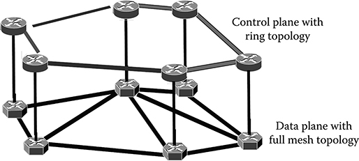
Figure 8.8 Communication structure dedicated to the control plane and its independence from the network on the data plane.
GMPLS uses generalized labels to perform routing of generalized label switched path (GLSP). In contrast to MPLS where labels merely represent network traffic, generalized labels represent network resources. For example, a generalized label on an optical link could identify a wavelength or a fiber, while on a packet-switched link, it would simply identify network traffic, just as in MPLS. In the lower layers, generalized labels are “virtual,” meaning that they are not inserted into the network traffic, but instead implied by the network resource being used (e.g., wavelength or fiber). This is necessary since neither packets nor frames are recognized at the lowest layers that GMPLS supports.
Generalizing the label format, the conventional MPLS label has been extended to 32 bits. The labeling of ports of routing equipment in GMPLS follows a particular convention that allows the control plane to identify the functionality of an equipment from the labeling of its ports.
In particular, the ports of routing equipments are classified in several classes that are as follows:
Fiber switching capable ports (FSC): These are the ports of equipment that can switch the entire fiber signal as a whole.
Wavelength switching capable ports (WSC): These are ports of equipment that can switch the single wavelength signal as a whole; since generally the port is occu-pied by a WDM system, a demultiplexer is expected so to divide at least a certain number of wavelengths (see the OADM structure in Chapter 6) so to be able to deal with each wavelength independently.
Time division multiplexing switching capable ports (TSC): These are the ports of equipment that can switch the single TDM frame; since generally the port is occupied by a complete TDM frame, a TDM demultiplexer is expected after the TSC.
Layer 2 frames switching capable ports (L2SC): These are essentially the ports of Ethernet equipments.
Packet switching capable ports (PSC): These are the ports of LSR and IP routers.
Every type of port has a different kind of generalized label so that the control plane can identify the type of port and so understand the equipment capability. An example of different types of ports is reported in Figure 8.9, where a core node hosting the overlay of an OXC and an LSP router is schematically shown. A few of the wavelength GLSPs transiting through the OXC are also sent to the LSR both for local dropping and for grooming, while other wavelength GLSP directly transit through the OXC.
This is a typical overlay node configuration, where the OXC ports are wavelength capable ports, while the LSR ports are packet capable ports. Finally ports with multiple switching capability can be defined, for example both PSC and WSC. When a GLSP requires the use of the port it also requires the functionality he needs among those available.
8.3.1 GMPLS Data Paths and Generalized Labels Hierarchy
A data path between two GLSRs is a different concept with respect to the GLSP. A GLSP consists of a sequence of consecutive labels, which, when swapped in a specific order, carries data from one point in a label switched network to another. In short, a GLSP is represented by the distributed state needed to send data along a specific route.

Figure 8.9 Different types of ports in the overlay of an OXC and an LSP router. (a) Shows a locally dropped GLSP, and (b) a pass-through GLSP. ΛSC indicates a wavelength switch capable port.
Because GLSPs might differ in link composition, an entity requesting labels for a GLSP needs to specify three major parameters: switching type, encoding type, and generalized payload-ID (G-PID). Switching type defines how an interface switches data. Because this is always expected to be known, a switching type needs only be specified for an interface with multiple switching capabilities.
Encoding type is needed to specify the specific encoding of the data associated with the GLSP. For example, data associated with an L2SC interface might be encoded as Ethernet.
The G-PID finally defines the client layer of the GLSP. In GMPLS, bidirectional GLSPs are considered the default. Bidirectional GLSPs are established through simultaneous label distribution in both directions. Since generalized labels are nonhierarchical, they do not stack. This is because some supported switching media cannot stack. Given an optical link, for example, it is not possible to encapsulate a wavelength in another and then get it back again.
In GMPLS, tunneling data through different layers is therefore based on GLSP nesting (i.e., encapsulating GLSPs within GLSPs). Nesting of GLSPs can be realized either within a single network layer or nesting GLSPs of a layer through a GLSP of another layer. Examples of the nesting system are reported in Figure 8.10.

Figure 8.10 Examples of Generalized Labels nesting: on the left (a) labels relative to different wavelength channels are nested into the fiber label, on the right (b) labels relative to different MPLS LSPs are nested into the wavelength path label.
In particular in Figure 8.10a, a set of wavelengths are nested into a fiber link by nesting the labels associated with wavelength channels resources into the label associated to the fiber channel.
This kind of nesting allows the wavelength channels to be considered as a single entity, to be routed always together, switched together and protected together. This kind of nesting is useful, for example, if a 100 Gbit/s virtual channel is transmitted as a group of four 20 Gbit/s channels. In this case, the association made through GLSPs nesting within the same layer allows the 100 Gbit/s channel to be recognized as a single entity by the network even if it is constituted by parallel wavelength channel.
Another case in which nesting wavelength into a fiber channel is useful when a client layer requires a SLA prescribing the same network traversing time for different wavelength channels. This can be achieved by nesting them into the same GLSP.
In Figure 8.10b the nesting of several MPLS LSPs into a lower layer wavelength channel is shown. Physically the GLSPs are multiplexed into a wavelength channel using OTN frame and GFP adaptation, under a logical point of view, in order to recognize that the GLSPs will travel the network in the same route, a GLSP is built nesting the individual layer two labels into a layer one label attached to the wavelength channel resources.
In general, ordering GLSPs hierarchically within a network layer requires that GLSP are encoded in a hierarchical way. A natural GLSP hierarchy can be established based on interface types and it is also the hierarchy used to build the examples of Figure 8.10. At the top of this hierarchy are FSC interfaces followed, in decreasing order, by LSC, TDM, L2SC, and PSC interfaces. This order is because wavelengths can be encapsulated within a fiber, time slots in wavelengths, data link layer frames in time slots, and finally network layer packets in data link layer frames. As such, an GLSP starting and ending on PSC interfaces can be nested within higher ordered GLSPs.
8.3.2 GMPLS Protocol Suite
Protocols of the GMPLS protocol suite can be divided into three distinct sets based on their functionality:
Routing protocols must be implemented by the MLCP to disseminate the network topology and its traffic engineered (TE) attributes. For this purpose, open shortest path first (OSPF) with TE extensions (OSPF-TE) or intermediate system to intermediate system (IS–IS) are currently defined. To account for multiple layers, however, GMPLS needs to add some minor extensions to these existing protocols. The GMPLS routing process using OSPF-TE is explained in the following sections.
Signaling protocols are concerned with establishing, maintaining, and removing network state (i.e., setting up and tearing down GLSPs). For signaling, GMPLS can use either Resource ReSerVation Protocol (RSVP) with TE extensions (RSVP-TE) or constraint-based routing-label distribution protocol (CR-LDP). Again, supporting multiple layers requires some extensions to existing protocols.
Link management is performed by a new protocol called the link management protocol (LMP), which has been defined within the GMPLS standard. LMP can be used by GMPLS network elements to discover and monitor their network link connectivity. To enable link discovery between an optical switch and an optical line system, LMP has been further extended, creating LMP-WDM.
In the following subsections, the working of the most used among the protocols of the GMPLS protocol suite will be described in some detail so as to give an idea of how GMPLS implements its functionalities.
8.3.2.1 Open Shortest Path First with Traffic Engineering
To enable automated configuration of the controlled network, GMPLS defines an intradomain routing process. Via this routing process, the network topology and its TE attributes are disseminated within the TE domain. This routing process is implemented using routing protocols specified for the MLCP. However, this routing process is not used for routing user traffic, but only for distributing information in the MLCP. To understand this point, we have to remember that, taking as an example the optical domain, user signals are organized in optical channels that are routed like circuits in that layer. Extensions to existing protocols necessary for this routing process were therefore created in the relevant IETF and OIF standards.
Essentially, with OSPF-TE, participating generalized label switched routers (GLSRs) first establish routing adjacencies by exchanging hello messages. After routing adjacencies have been established, the GLSRs then synchronize their link state databases. This is done by exchanging database description packets.
The database description packets contain at least one database structure referred to as a link state advertisement (LSA). Different LSA types exist but all share a common 20-byte header whose structure is shown in Figure 8.11.
The primary OSPF-TE operation is to flood LSAs throughout the MLCP domain by appending them to “link state update” messages periodically sent between adjacent GLSRs. To avoid interference with any ordinary routing processes, a TE LSA is made opaque. Such an opaque LSA is a special type of LSA only processed by specific applications (e.g., the GMPLS routing process). By extending the link state database with TE information, a traffic engineering database (TED) is produced. From this TED, a network graph with traffic engineering content can be computed. Constructing a TE network graph is necessary to provide input for the constraint-based algorithms subsequently used to compute network paths.
When flooding LSAs, each OSPF-TE routing message contains a common 24-byte header, which is used to forward it. This routing message header includes information about message type, addressing, and integrity. Within this header, LSAs are then encapsulated and specific payloads appended to each LSA. In order to enable advertisement of TE attributes in opaque LSAs, the LSA payload consists of type-lengthvalue (TLV) records. These are information records composed by three fields: two 2-byte fields, the “Type” and “Length” fields, and a variable length field, the “Value” field. Using TLVs, router addresses and TE links can be expressed.
In GMPLS, if an advertising router is reachable, a “router address”-TLV can be used to describe a network address at which this router (i.e., GLSR) can always be reached. In turn, the “link”-TLV can be used to abstract advertised TE links. Multiple TE attributes can be represented on each link using fields that are related to the “link”-TLV address, which are called sub-TLV. Thus, in the case of a link address, the TLV appears as the first field and pointer of a bigger record containing all the information that are needed to the MLCP about the link in order to perform routing operations.

Figure 8.11 Common 20-byte header of OSPF-TE LSA messages.
Table 8.1 Record Containing the Information Needed to the MLCP to Perform Routing Operations
Sub-TLV Name |
Type |
Length |
Value |
Link local/remote identifiers |
11 |
8 bytes |
2 × 4 bytes local/remote link identifiers |
Link protection type |
14 |
4 bytes |
1 byte for link protection (3 bytes reserved) |
Interface switching capability descriptor |
15 |
Variable |
Minimum 36 bytes for ISCD information |
Shared risk link group |
16 |
Variable |
N × 4 bytes for link SRLG identification |
The structure of this bigger record is reported in Table 8.1. Two links attributes of Table 8.1 are worth a comment. The first is the last attribute of the record, advertising that the link is part of a shared risk link group (SRLG). An SRLG is a group of links that will fail contemporary when a certain type of failure happens.
As an example, we can look at Figure 8.12, where typical situations are represented. Physical fiber connections are routed through multifiber cables and links having different destinations are built over a cable structure that generally has been deployed without any knowledge of the overlay network.
Thus, also links that have completely different source and destinations can share in a part of their path the same fiber cable. If the cable is cut, for example, due to civil works, all those links goes down, thus they have to be put together in the same SRLG.
The definition of SRLGs is fundamental when defining protection or restoration strategies. As a matter of fact, when the protection capacity is preprovisioned, it is fundamental to avoid that a link is protected by another link in the same SRLG, otherwise a single failure could hit both working and protection link, making the protection useless. In the case of restoration, when routing of the restoration path is performed, also links in the same SRLG has to be avoided. This is why the SRLG is indicated among the information related to the routing protocol.

Figure 8.12 Concept of SRLG.
The second field that is worth a comment is the interface switching capable description. It is clear that a link will terminate on the same type of interfaces and this field let the routing protocol know what kind of interfaces there are at the link extremes. During GLSPs, this information can be very useful to balance sparing of higher layer interface use achieved by transparent pass-through of the traffic not destined to the node with transmission resources sparing achieved by grooming (see Section 8.4: Design and Optimization of ASON/GMPLS Networks).
Once the OSPF-TE has flooded the network and created all the nodes capable of routing GLSPs, a database of the routing area topology, the OSPF-TE routing engine can start every time there is a GLSP to route either if it is a new path or it is needed to carry out restoration of a failed path.
The OSPF-TE routing engine is based on the so called Dijkstra algorithm (from the name of the inventor), which is an algorithm that is able to find in a graph with tagged links the shortest path between two given nodes. In GMPLS, what should be the tagging of the links of the network is not prescribed in a mandatory way; generally every link is associated to its length and the GLSP are routed along the shortest path in term of kilometers. This is a reasonable solution since the cost of a DWDM system is roughly proportional to its length due to the presence of EDFA sites. Thus, since if I occupy preferably the shortest links I will have to upgrade them sooner, this strategy tends to minimize the cost of network upgrades.
However, in specific situations, it is possible to tag the network links with other numbers. For example, a competitive carrier leasing fibers from another company could tag the link with the leasing price so to use always the cheaper links. This direct routing through the topology of the network with the Dijkstra algorithm becomes increasingly complex while the network dimension increases, so that the routing process has to be simplified in some way if OSPF-TE has to scale up to the dimension of an incumbent carrier network. The solution to this problem is the division of the network in routing areas and the execution of the routing in a hierarchical manner.
In particular, OSPF-TE individuates in the network a set of routing entities (GLSR) that are suitably distributed to constitute the so-called network backbone. All the other GLSRs are divided in routing areas constituted by nearby nodes. Each distinct routing area has to be in contact with the backbone at least in two points to assure effective network survivability. An example of this hierarchical organization of the network is reported in Figure 8.13.
Staring from this structure, a new higher level topology (the area topology) is constructed substituting all the routing areas with virtual nodes; this new topology has for sure at least interconnection degree equal to 2 due to the presence of the backbone and to the way in which the areas have been constructed.
The routing between nodes in different areas is performed in two steps: first the route is individuated in the area topology, then, knowing for each traversed areas the incoming and the outcoming nodes, the path route is specified also within areas.
8.3.2.2 IS–IS Routing Protocol
IS–IS is designed and optimized to provide routing within a single network domain, while passage through a domain interface for multidomain GLSPs have to be realized with a different protocol (e.g., the BGP, see Chapter 3, Table 3.1 IP protocol suite). IS–IS is based on the concept of routing domains. An IS–IS routing domain is a network in which all the equipments that perform GLSP routing run the integrated IS–IS routing protocol to support intradomain exchange of routing information.

Figure 8.13 GMPLS partition of the network in routing areas and backbone. On the right of the figure the virtual topology where each routing area is represented by a virtual node is represented.
The underlying goal is to achieve consistent routing information within a domain by having identical link-state databases on all routing entities in that area. Hence, all routing entities in an area are required to be configured in the same way.
IS–IS protocol supports a two-level hierarchy for managing and scaling routing in large networks. A network domain can be divided into small segments known as areas. The topology resulting from the substitution of each area with a virtual node and each connection between nodes in different areas with a connection between the corresponding virtual nodes is called area topology. This construction allows hierarchical routing to be carried out within the domain.
This means that the routing between nodes in different areas is performed in two steps: first the route is individuated in the area topology, then, knowing for each traversed areas the incoming and the outcoming nodes, the path route is specified also within areas. Following the same network representation, IS–IS routing entities are hierarchically ordered depending on their ability to route GLSPs only within their area or also toward other routing areas. In particular routing entities that are only able to route paths within their area are called Level 1 routers (not to confound with Layer 1 entities; this is a specific IS–IS hierarchy completely different from the network layering).
Following the same criterion, routing entities that can route GLSPs only between virtual nodes that represents routing areas are called Level 2 routers (or inter area routers) and finally routing entities that are able to route GLSPs both inside the area and between different areas are considered logically as a superposition of communicating Level 1 and Level 2 routers and are called Level 1–2 routers.
Level 2 routers are interarea routers that can only form relationships with other Level 2 routers; in other words, they can route through the area topology constituted by virtual nodes representing the routing areas. Similarly Level 1 routers can exchange information only with other Level 1 routers. Level 1–2 routers exchange information with both levels and are used to connect the interarea routers with the intraarea routers.
Integrated IS–IS uses the legacy CLNP node-based addresses [35–37] to identify routers even in pure IP environments. The CLNP addresses, which are known as network service access points (NSAPs), are made up of three components: an area identifier (area ID) prefix, followed by a system identifier (SysID), and an N-selector. The N-selector refers to the network service user, such as a transport protocol or the routing layer.
A group of routing entities belongs to the same area if they share a common area ID. Note that all routing entities in an IS–IS domain must be associated with a single physical area, which is determined by the area ID in the router address. IS–IS packets can be divided into three categories:
Hello packets are used to establish and maintain adjacencies between IS–IS neighbors.
Link-state packets are used to distribute routing information between IS–IS nodes.
Sequence number packets are used to control distribution of linkstate packets, essentially providing mechanisms for synchronization of the distributed link-state databases on the routers in an IS-IS routing area.
Each type of IS–IS packet is made up of a header and a number of optional variable-length fields organized in records and containing specific routing-related information. The variable length fields are called TLV as in the case of the OSPF-TE from the form of the record that is organized into three fields: type, length, and value.
Each variable-length field has a 1-byte type label (the Type field) that describes the information it contains. The second field is a length information that contains the length of the third field whose content is the specific information that is carried by the TLV (see Table 8.1 for examples). The different types of IS–IS packets have a slightly different composition of the header, but the first 8 bytes are repeated in all packets. Each type of packet then has its own set of additional header fields, which are followed by TLVs.
Table 8.2 lists TLVs specified in ISO 10589 while Table 8.3 lists the TLVs introduced by IETF in RFC 1195.
Enhancements to the original IS–IS protocol are normally achieved through the introduction of new TLV fields. Note that a key strength of the IS–IS protocol design lies in the ease of extension through the introduction of new TLVs rather than new packet types.
The routing layer functions provided by the IS–IS protocol can be grouped into two main categories: subnetwork-dependent functions and subnetwork-independent functions.
Table 8.2 List of TLVs Specified in ISO 10589

Table 8.3 List of the TLVs Introduced by IETF in RFC 1195

The subnetwork-dependent functions involve operations for detecting, forming, and maintaining routing adjacencies with neighboring routing entities over various types of interconnecting network links. The subnetwork-independent functions provide the capabilities for exchange and processing of routing information and related control information between adjacent routers as validated by the subnetwork-dependent functions.
The routing information base is composed of two databases that are central to the operation of IS–IS: the link-state database and the forwarding database. The link-state database is fed with routing information by the update process. The update process generates local link-state information, based on the adjacency database built by the subnetwork- dependent functions, which the router advertises to all its neighbors in link-state packets.
A routing entity also receive similar link-state information from every adjacent neighbor, keeps copies of GLSPs received, and readvertises them to other neighbors. Routing entities in an area maintain identical link-state databases, which are synchronized using SNPs. This means that routing entities in an area will have identical views of the area topology, which is necessary for routing consistency within the area. The decision process creates the forwarding database by running the Dijkstra algorithm on the link-state database so selecting for each GLSP and for the forward of each control packet the shortest path in terms of whatever weight is associated to each network link in the topology database.
The IS–IS forwarding database, which is made up of only best IS–IS routes, is fed into the routing information base.
8.3.2.3 Brief Comparison between OSPF-TE and IS–IS
IS–IS and OSPF-TE are link-state protocols, that is routing protocols that perform routing on the ground of information on the state of the links of the network that is derived from a map of the network topology that each routing network element stores and updates using the protocol flooding functionality. Moreover, OSPF-TE and IS–IS have several other common characteristics:
They use the Dijkstra algorithm for computing the best path through the network.
They allow any link tag as weight for the Dijkstra calculation.
They exchange via protocol packets records composed by sets of TVL fields that describe the characteristics of the link they are advertising.
They use the concept of subnetwork and virtual node to leverage on hierarchical routing to simplify routing tables and routing computation.
They can use multicast to discover neighboring routing equipment using hello packets.
They can support authentication of routing updates.
As a result, OSPF-TE and IS–IS are conceptually similar.
While OSPF-TE is natively built to route IP and is itself a Layer 3 protocol that runs on top of IP, so that OSPF-TE packets are a particular type of IP packets, IS–IS is natively an OSI network layer protocol (it is at the same layer as CLNS [35–37]), a fact that may have allowed OSPF to be more widely used. IS–IS does not use IP to carry routing information messages and its packets are not IP packets.
In line of principle IS–IS does not need IP addressing, even if, since some form of addressing is needed to route GLSPs through the network, in practical applications IP addressing is almost always used in conjunction with IS–IS.
Routing entities of a network implementing IS–IS build a topological representation of the network. This map indicates the subnetworks that each IS–IS enabled equipment can reach, and the lowest cost (shortest) path to any subnetwork is used to forward IS–IS packets and to route GLSPs.
Due to its structure, IS–IS is also more scalable that OSPF-TE: given the same set of resources, IS–IS can support more routing entities in an area with respect to OSPF-TE. IS–IS differs from OSPF-TE also in the way that “routing areas” are defined and interarea routing is performed. No hierarchy similar to that present in IS–IS is present in OSPF-TE, whose routing entities are all on the same ground, capable of interarea or intraarea routing when it is needed.
In OSPF, areas are delineated on the interface such that an area border router (ABR) is actually in two or more areas at once, effectively creating the borders between areas inside the ABR, whereas in IS–IS area borders are in between routers, designated as Level 2 or Level 1–2. The result is that an IS–IS router is only ever a part of a single area. IS–IS also does not require the backbone (or Area Zero as it is sometimes called) through which all interarea traffic must pass, while OSPF-TE needs this definition to manage multiarea routing domains.
The logical view is that OSPF creates something of a spider web or star topology of many areas all attached directly to area zero and IS–IS by contrast creates a logical topology of a backbone of Level 2 routers with branches of Level 1–2 and Level 1 routers forming the individual areas.
8.3.2.4 Resource Reservation Protocol with Traffic Engineering Extensions
Because RSVP-TE inherits its design from the RSVP protocol, it is based on distributing various signaling objects. These signaling objects have been grouped. These groups contain mandatory and optional signaling objects; encapsulating the groups with a common header, distinct signaling messages are created.
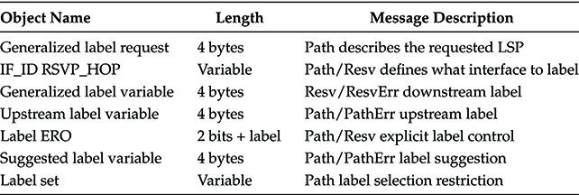
When a GLSR receives a signaling message, the resident objects are examined and interpreted based upon the message type indicated by the common header. Extending the RSVP-TE protocol for GMPLS was thus a matter of generalizing existing signaling objects, including some new objects that are reported in Table 8.4, and adding some minor signaling enhancements.
Considering the RSVP-TE protocol with GMPLS extensions for signaling, each signaling message contains a common 8-byte header. The common header defines the message type followed by the encapsulated objects. Encapsulated objects are of variable length and contain a 4-byte header defining the object length, class, and type within class.
Table 8.4 New Objects Introduced in the Adaptation of RSVP-TE for the GMPLS
The first signaling activity of RSVP-TE is to distribute the labels that are used in the GLSPs. The mechanism used by RSVP-TE is downstream-on-demand label distribution: this means that upstream GLSRs request downstream GLSRs to select labels for the links connecting them. In this way, each GLSR acknowledges a request to install an GLSP, forward the request to the next downstream hop, and awaits the response.
As a response is returned upstream, the GLSR can install a cross-connection (i.e., state describing ingoing and outgoing labeltointerface mappings and associated network resources) for this GLSP. Here, downstream is defined as the direction from GLSP ingress to GLSP egress for a unidirectional GLSP. In the case a bidirectional GLSP is to be set up, this is done by contemporary setup of two unidirectional GLSPs.
Once all the labels are assigned, the GLSP can be set up. As a matter of fact, GLSR can route the signal incoming from an input port toward the output port with the same label and the GLSP is identified in the path topology through the vectors whose elements are the labels of the links traversed by the path in the correct order.
As for all signaling protocols, RSVP-TE operation is composed of three main functions:
GLSP setup that is carried out via labels distribution.
GLSP management, a function composed by various elements among which error management is probably the most important.
GLSP tear down that is carried out by labels removal.
8.3.2.4.1 GLSP Setup
Establishing bidirectional GLSPs employing RSVP-TE for signaling requires full sets of Path and Reservation (Resv) messages to be exchanged between two GLSRs. This procedure is sketched in Figure 8.14.
Initially, a sender GLSR (GLSP ingress) requests a GLSP to be set up by sending a Path message downstream to the next hop. This Path message contains an UPSTREAM_LABEL object defining the label to use in the upstream direction, objects describing the data flow, and a GENERALIZED_LABEL_REQUEST object for requesting the GLSP.
If the Path message is successfully received, the next hop then reserves path state to enable correct signaling of returning Resv messages and saves the upstream label. The next hop then selects its own upstream label, creates state for the upstream direction, replaces the upstream label in the Path message, and passes it on downstream to the next hop. This procedure is repeated until the next hop is the receiver GLSR (GLSP egress). The GLSP has now been established in the upstream direction, but no state has been saved in the downstream direction. Consequently, the receiver GLSR selects a downstream label and returns a Resv message upstream. This Resv message mimics the Path message, but inserts a GENERALIZED_LABEL object defining the selected downstream label. If the Resv message is received successfully, the previous hop (the signaling direction has changed) then sets state for the downstream direction, replaces the downstream label with its own selected label, and passes the Resv message further upstream.

Figure 8.14 Establishment of a bidirectional GLSPs employing RSVP-TE for signaling; full sets of Path and Reservation (Resv) messages are exchanged between two GLSRs.
This procedure is repeated until the sender GLSR successfully receives the Resv message corresponding to a dispatched Path message. Now, the request has been fully established and is ready to tunnel data in both directions. This procedure is shown in Figure 8.14 while the final aspect of the GLSP as a cascade of labels is sketched in Figure 8.15.
It is possible using RSVP-TE to route a certain GLSP on a preassigner route. This is needed in order to traffic engineer the network. As a matter of fact, if a generic network is considered, the OSPF routing criterion used both by OSPF-TE and IS–IS is a suboptimum routing strategy. It is not difficult to find examples where routing a few GLSPs along a longer path allows a more efficient exploitation of the network resources.

Figure 8.15 Generalized Label Assignment for a bidirectional GLSP.

Figure 8.16 An example of suboptimum routing performed with OSPF-TE. Each link between a couple of GLSR is assumed to have enough capacity to support only two GLSPs.
Such an example is provided in Figure 8.16. Here a network of five nodes with an incomplete mesh connection is represented. For simplicity let us image that each link is physi-cally realized with a WDM system with two wavelengths and that all the wavelengths have the same capacity, which we assume equal to 1.
Let us also imagine to tag every link with a weight that is the “cost” of using a wavelength along that link. We could also think that the weight is the link length and that it is assumed as a cost due to the fact that WDM systems have a cost roughly proportional to length.
Such GLSPs, each of which for simplicity is imaging to have unitary capacity, so that it completely uses a single wavelength, correspond to traffic requests arriving at the network control plane one after the other so that they are routed in successive times and when one of them is routed the network control plane does not know what set of traffic requests will arrive in the future.
In this dynamic situation, typical of GMPLS networks, the OSPF-TE protocol produces the routing that is listed in the first routing table in Figure 8.16. Naturally, also IS–IS would have produced the same routing due to the use of the same routing algorithm and to the fact that this simple network is a single routing area. The overall cost of the routing is obtained by adding together all the costs of the used wavelengths and it is reported in the figure as 335.
However, it is not difficult to see that at least one alternative routing exists having a lesser cost, reported as 325 in Figure 8.16. This routing is based on the knowledge of the whole traffic request, that in reality the control plane does not have, and achieve a lesser overall cost by using two times the link DC even if it is the most expensive of the network, and obtaining in return the possibility to better distribute the weights of all the GLSPs.
This example shows that if the traffic is completely known, routing solutions better, and sometimes much better, then the routing produced by protocols like OSPF-TE or IS–IS can be produced. As a consequence, generally a traffic engineering tool is incorporated into the network manager. It has the scope to route the traffic that the network is managing in an optimized way with respect to OSPF.

Figure 8.17 RSVP-TE message structure.
From time to time, the deviation of the real routing achieved by OSPF-TE or IS–IS from the solution found through the traffic engineering tool becomes important and it is man-datory to reroute a certain number of GLSPs to optimize the network and avoid waste of resources.
In order do that is must be possible to force the routing of a GLSP along a predeter-mined route. Using RSVP-TE this can be done introducing in the Path and Resv messages exchanged during GLSP state installation the EXPLICIT_ROUTE object (ERO, see Figure 8.17).
When used in Path messages, the ERO describes the next and previous hop for any GLSR along the explicit route. When signaling paths explicitly use an ERO, path state is not needed to indicate a reverse route, since returning Resv messages can instead be routed based upon the ERO. In practice, when dealing with large networks composed by many layers and a huge number of paths, the use of automatic routing protocols to route GLSPs is so inefficient and explicit routing would be so frequent that there is a proposal to use rout-ing protocols to route packets in the control plane and adopting explicit routing through ERO as the default to route GLSPs.
While the earlier description of the signaling procedures presumed that no errors occurred during signaling, this is unlikely to always be true. Thus, a need for error han-dling messages arises. When errors occur, PathErr or ResvErr messages can therefore be signaled.
A PathErr message indicates an error in processing a Path message and is sent upstream toward the GLSP ingress. Similarly, a ResvErr message indicates an error in processing a Resv message and is sent downstream toward the GLSP egress. A GLSR receiving an error message may try to correct the error itself, if minor, or pass it further on.
8.3.2.4.2 GLSP Tear Down
RSVP-TE is a soft-state protocol. This means that it continuously sends messages refresh-ing timers associated with installed state. Originally designed for MPLS, the “softness” is somewhat reduced in GMPLS, however timers are still implemented.
GLSP state removal can be triggered in two ways: when a timer expires in a GLSR or by some external mechanism (e.g., manual operator or management system). To remove GLSP state using RSVP-TE, PathTear or PathErr messages are dispatched. A PathTear message is dispatched downstream following the path of a Path message, while a PathErr message is sent upstream following the path of a Resv message.
As these messages are processed by GLSRs they immediately clear, or partially clear, the GLSP state. This enhancement is specific to GMPLS and enables the GLSP egress and intermediate GLSRs to initiate GLSP state removal. Using the PathErr message for clear-ing state, a flag introduced by GMPLS is set to indicate that path state is no longer valid. This means that GMPLS can tear down GLSP state in both directions (both upstream and downstream). Additionally, GMPLS provides rapid error notification via the Notify message (Figure 8.18).

Figure 8.18 GLSP Tear down procedure with RSVP-TE.
The Notify message can be used to inform an GLSP ingress or egress of errors, enabling them to initiate state removal in the place of an intermediate GLSR. Although the PathErr message is, strictly speaking, not needed, it can increase signaling efficiency by eliminat-ing the need for notification.
8.3.2.5 Constrained Routing Label Distribution Protocol
In the GMPLS network, GLSR must agree on the meaning of the labels used to for-ward traffic between and through them. This signaling operation can be performed by RSVP-TE, but a group of equipment vendors has pushed another protocol. The CR-LDP is an extension of the protocol used for the same scope in MPLS: the Label Distribution Protocol (LDP).
CR-LDP is a new protocol that defines a set of procedures and messages by which one GLSR informs another of the label bindings it has made. This implicitly advertises the GLSP setup since it is performed by assigning label bindings across GLSRs. The idea below the introduction in the GMPLS protocol suite of this extended protocol is to incorporate traffic engineering capabilities into a well-known protocol widely used in MPLS networks. The traffic engineering requirements are met by extending LDP for support of constraint-based routed label switched paths (also sometimes called CR-GLSPs).
Like any other GLSP, CR-GLSP is a path through a GMPLS network. The difference is that while other paths are setup based on information in routing tables or from a direct intervention of the management system, the CR-LDP constraint-based route is calculated at one point at the edge of network based on criteria including but not limited to explicit route constraints or QoS constraints.
The GLSR uses CR-LDP to establish LSPs through a network by mapping network layer routing information directly to data-link layer switched paths. A Forwarding Equivalence Class (FEC) is associated with each GLSP created. This FEC specifies which type of information is mapped to that GLSP and can be used for assuring the needed QoS during the GLSP setup.
Two GLSR which use CRT-LDP to exchange label mapping information are known as CR-LDP peers and they have a CR-LDP session between them. In a single session, each peer is able to learn about the other label mappings, that is, the protocol is bi-directional.
There are four types of CR-LDP messages:
Session messages
Discovery messages
Advertisement messages
Notification messages
Session messages are used to manage the CR-LDP section through the standard section management steps:
Section setup through handshaking between the GLSR at the section ends
Section monitoring
Section teardown through another specific handshaking
Using discovery messages, the GLSRs announce their presence in the network by sending Hello messages periodically. This Hello message is transmitted as a UDP packet allocated into a GLSP that always exists when a physical capacity is deployed along a link in order to convey at least control plane messages.
When a new session must be established, the Hello message is sent over TCP to have a better control of the session opening procedure. Apart from the Discovery messages all other messages are sent over TCP. Advertisement messages are used to disseminate across the network the discovery of new network entities or other modifications in the network topology that influences the labels distribution. For example, if a link fails, this has to be eliminated from the topology map that each GLSR has in the routing engine. This is discovered by processing the absence of response to all the Hello messages that are directed toward that link and is advertised to all the network routing entities via advertisement messages. The notification messages signal errors and other events of interest. There are two kinds of notification messages:
Error notifications: these signal fatal errors and cause termination of the session
Advisory notifications: these are used to pass on GLSR information about the CR-LDP session or the status of some previous message received from the peer
All CR-LDP messages have a common structure that uses a TLV encoding scheme. This TLV encoding is used to encode much of the information carried in CR-LDP messages. The Value part of a TLV-encoded object may itself contain one or more TLVs. Messages are sent as CR-LDP PDUs. Each PDU can contain more than one CR-LDP message. Each CR-LDP PDU is an CR-LDP header followed by one or more CR-LDP message.
8.3.2.6 Comparison between RSVP-TE and CR-LDP
From the brief description we have done, it is quite evident that RSVP-TE and CD-LDP have almost all the same functionalities, even if they are constructed using different criteria. Thus a comparison between the two protocols, which are obviously alternative in a particular implementation of GMPLS, can be useful.
The summary of this comparison is mainly derived from Ref. [3].
Transport Protocol: The first difference between CR-LDP and RSVP is the choice of transport protocol used to distribute the label requests. RSVP uses connectionless raw IP or UDP encapsulation for message exchange, whereas CR-LDP uses UDP only to discover GMPLS peers and uses connection-oriented TCP sessions to distribute label requests.
Security: Once the path has been established and the data is being forwarded, the frame is no longer visible to the management or control plane software at the upper layers of the network. There is minimal chance that unauthorized individuals will be able to sniff or ruin the data or even redirect them toward an unintended destination.
Data is only allowed to enter and exit the GLSP at locations authorized and configured by the control plane. Both CR-LDP and RSVP-TE have the support of MD5 signature password and authentication. CR-LDP uses TCP/IP services, which is vulnerable to denial of service attacks; therefore, any in-between errors are reported immediately.
RSVP-TE uses UDP services and the IETF standard to specify an authentication and policy control. This allows the originator of the messages to be verified (e.g., using MD5) and makes it possible to police unauthorized or malicious reservation of resources. Similar features could be defined for CR-LDP but the connection-oriented nature of the TCP session makes this less important.
8.3.2.6.1 Protocol Type
RSVP-TE is a soft state protocol. After initial GLSP setup process, refresh messages must be periodically exchanged to notify the peers that the connection is still desired. State refreshes help to make sure that GLSP state is properly synchronized between adjacent nodes, procedure that is required by the fact that RSVP-TE uses IP datagrams, so that control messages may be lost without notification.
Periodic refresh messages imply the refresh overhead: this is a sort of weakness in the protocol that makes a bit more difficult to scale it to large networks. A proposed solution to reduce the refresh messages number and the bandwidth they require from the control plane communication structure is bundling many refresh messages together. This reduces the traffic volume but the processing time is still the same.
CR-LDP is referred to as a hard state protocol. This means that all the information is exchanged at the initial setup time, and no additional information is exchanged between GLSR until the GLSP is torn down. No refresh message is needed due to the use of TCP. When a GLSP is no longer needed, decision that can be taken by the client that has delivered the request to the control plane or by the central management system, messages must be exchanged notifying all routers that the GLSP is down and the corresponding allocated resources are now free.
8.3.2.6.2 Surviving Capability in Front of Control Plane Communication Failures
RSVP-TE is based on datagram transmission of service packets using UDP; thus it is intrinsically robust versus failures in the communication capacity available for the control plane. On the other hand, CR-LDP is in principle more vulnerable versus such failure. However, this vulnerability is not always a real weakness of the protocol, since survivability strategies are generally adopted in the control plane communication network.
8.3.2.7 Line Management Protocol
The last key protocol of the GMPLS suite is the line management protocol; it is a pointto-point protocol that has the role of managing the link between adjacent nodes. As a matter of fact, traditional IP and MPLS protocol suite leverages on the physical layer to manage physical links. On the contrary, GMPLS cannot do that, since it is in charge of the entire network layering, thus a new protocol has been invented for this role. In particular, referring to an optical link, for generality with several WDM channels, LMP is aimed at the following tasks:
Control-channel management
Link connectivity verification
Link property correlation
Fault management
8.3.2.7.1 Control Channel Management
In order to set up a channel, the control plane must know the IP address on the far end the channel either due to a manual configuration or for automatic discovery. This role, which is a typical point-to-point function relative to a specific link, is performed by the LMP via Config/ConfigAck messages exchange. This procedure discovers peer’s IP address and establishes LMP adjacency relationship automatically. Adjacency relationship requires at least one bidirectional control channel (multiple can be used simultaneously) between peers.
In order to run the control plane through the link and establish an adjacency relationship, a control channel traversing the link is needed. This is generally defined at the control plane level by a set of parameters that are negotiated by LMP during the adjacency discovery. Once set up, the control channel maintenance is done by LMP by periodic Hello messages.
8.3.2.7.2 Link Connectivity Verification
A GLSR knows the local address (ID) for data links that connect its ports to the ports of a peer GLSR. In the absence of a suitable mechanism, the GLSR does not know how a peer identifies the same data links and has no a priori information about the state of the data links. Link IDs mapping between peers should be made in order to have a common unambiguous association between a link and a link ID and in order to understand signaling messages received from a peer where the link ID is that assigned from the peer.
Links ID association is performed by the LMP using test message contains two key parameters: sender’s local data_link_ID and Verify_ID; the first is the ID that the GLSR assigns to a link, the second is the request done to the GLSR on the other side of the link: verify the link ID correspondence. Verify_ID also contains the GLSR ID.
The GLSR on the other side of the link looks at Verify_ID to understand from which adjacent GLSR the message comes from. The peer answers with TestStatusSuccess that contains peer’s local data link ID and the data link ID from the Test message.
8.3.2.7.3 Link Property Correlation
This is a process of synchronizing properties of data channels (e.g., supported switching and encoding types, maximum bandwidth that can be reserved, etc.) between peers and aggregation of data channels to form one TE link done by exchange of messages containing the parameters LinkSummary and LinkSummaryAck or LinkSummaryNack (if the peer does not agree on some parameters). In this case a new LinkSummary message is sent after LinkSummaryNack.
8.3.2.7.4 Fault Management
Since LMP is the tool that GMPLS control plane uses to manage the single point-to-point link, the procedure to localize a failure and to issue a notification message to the GLSR on the other side of the failed link starts, if it is the case, the restoration mechanism is located within the functionalities of LMP. To locate a fault up to a particular link between adjacent nodes, a downstream node (in terms of data flow) that detects data link failures will send a ChannelStatus message to notify its upstream peer.
8.4 Design and Optimization of ASON/GMPLS Networks
The introduction of the ASON/GMPLS control plane is a real revolution in the carriers network, a new paradigm that substitutes the idea of centrally controlled network that was the strong point of the introduction of SDH/SONET. This evolution is strictly related to the gradual change in the service bundles that carriers offer to customers and consequently in the characteristics of the traffic routed through the network [4,5].
In particular the traffic is getting more dynamic and the operation of setting up a connection or reroute a connection is no more a rare event. Moreover, and probably more important, it is much more difficult to foresee the evolution of future traffic. In the telephone era, when incumbent carriers were monopolist almost everywhere in the world, the traffic was strictly related to the population and to the well-known statistical characteristics of the telephone call.
With the dominant role of data services and the mobility of the customers due to the competition of different carriers and to the variety of service offering, there is no more a known statistical distribution that helps carrier planners to forecast the traffic behavior. As a consequence, the network design has to be adapted to the new paradigm, where unpredictable traffic is routed on an automatically managed network.
8.4.1 Detailed Example: Design Target and Issues
Since the design problem for an ASON/GMPLS network is really complex comprising a great number of elements, in this section, we will carry out in detail a simple example, in order to clarify some of the main issues in designing such a network.
We will not be so formal in defining performance evaluation parameters and design procedures, and a more precise discussion of these points will be carried out in Sections 8.5 and 8.6. The main task of this section is to give a feeling of the main aspects and of the complexity of the problem working on a very simple example.
The network we will consider in this example is a multilayer network, like the ASON/GMPLS networks. We will assume for simplicity that a DWDM transport layer based on electrical core OXCs has a single client layer, an IP network. We will also assume that the IP network is composed of LSRs and managed by an MPLS control plane, and that the overlay model defined by the GMPLS standard is implemented for the overall control plane. This means that the general network node is equipped as in Figure 8.19, with an LSR connected to an electrical core OXC via a UNI interface.
The starting point is the physical topology constituted by buildings where it is possible to place network nodes and fiber cables as represented in Figure 8.20.
At the beginning, we will assume that the traffic to be routed through the network is known and that the design consists of deploying equipment on the given topology in an optimized way to support the traffic. In a second step, we will see what happens if the traffic is not known, but it is known only as traffic statistics.
To simplify the approach, we will assume that all the MPLS layer LSPs to be set-up have the same capacity and that we will set equal to one to normalize transmission capacities.

Figure 8.19 Scheme of the two layer node considered in the example of network dimensioning.

Figure 8.20 Physical topology, traffic matrix, and link lengths of the network considered in the example of dimensioning.
In this normalized measurement unit, a wavelength, structured with the OTN frame, has capacity w ≥ 1.
The last element that is needed to characterize the topology is the distance matrix [L], which is the matrix whose elements are the length of the physical links connecting the nodes. We are considering obviously physical length, which takes into account the real structure of the cable system and thus that can be used to design transmission systems. The value we will assume in our example for the normalized lengths of the links are reported in Figure 8.20.
The traffic also, if it is a priori known, can be represented with the matrix [T] of the MPLS layer LSPs routing requests, whose value for our exercise is also reported near the network topology in Figure 8.20. To deploy equipment in an optimized way means to deploy the minimum cost network that can manage with the required reliability and QoS the given traffic. For the moment we do not consider QoS, even if this is in general an important point of the design.
In order to minimize the cost, a cost model has to be done for all the equipment that is present in the network.
We will choose a simple model, in line with the nature of this example:
The cost of LSR will be proportional to the number of ports (λj will indicate the number of ports of the LSR in the node j, if λj = 0 no router is present). The proportionality constant (unitary cost of one LSR port) will be indicated as χL.
The cost of OXC will be proportional to the number of ports (κj will indicate the number of ports of the OXC in the node j, if κj = 0 no equipment is present since in the overlay model no LSR can be deployed without the transport layer switch). The proportionality constant (unitary cost of one OXC port) will be indicated with χx.
The cost of the WDM will be composed by two addenda:
The first term represents transponders and is proportional to the number of wavelength (ωjn and will indicate the number of wavelength of the WDM on the link jn, if ωjn = 0 no WDM is present). The proportionality constant (unitary cost of one WDM wavelength) will be indicated with χw.
The second is proportional to the length ljn and represents the infrastructure (amplifiers and so on). The proportionality constant (cost of a unit length WDM infrastructure) will be indicated as χ0.
With this simple model we can try to optimize the network.
In particular, we will adopt two different optimization criteria that correspond to different balances between the cost of the transport layer and the cost of the packet layer: we will try to minimize first the cost of the nodes and then the cost of the links. In both cases we will do the realistic hypothesis that χx < χL, that is, the port of an OXC is cheaper than a port of an LSR.
8.4.1.1 Basic Examples of Network Design
In this section, we will start to introduce a few basic elements of ASON/GMPLS network design neglecting two key elements: The uncertainty on the traffic forecast and the need of designing the network so as to allow some survivability strategy.
Even if these elements are key points in a real network design, at the first moment, they would mask more fundamental issues like transparent pass-through versus groomingbased design, mesh versus hub design, and finally the importance of linear cost models. In the next section, we will reconsider the design example of this section adding design for survivability and design in uncertain traffic conditions. Section 8.4.1 is intended as a preparation to the more formal discussion about ASON/GMPLS network design that we will carry out from Sections 8.4.2 through 8.4.4.
8.4.1.1.1 Node Cost Minimization and Shortest Possible WDM Links
Since we know the traffic to be routed, but we do not know the order in which the requests will arrive, we can imagine to route the GLSPs in an optimized way and then to use the constrained routing to reproduce such optimized configuration whatever be the order of the requests.
In order to minimize the node cost and, in situations in which the node cost does not change, to have the shortest possible WDM links, we will proceed as follows:
GLSPs and OXC have to be installed in every node.
WDM links are installed in links ℓ23, ℓ12, ℓ34, ℓ14 so to form a sort of ring. Link between nodes 2 and 4 is not equipped.
The GLSP between nodes 2 and 3 is routed through the direct route that is also the shortest route of the graph.
The GLSPs from nodes 1 to 3 are routed through node 4 in order to have a WDM link of length 6 instead of 7 that is the length of the connection 1 → 2 → 3.
The GLSPs from 3 to 4 are also routed through the direct route.
The LSR ports are used only to generate and terminate local GLSPs and the transport is completely performed at the WDM layer. When an GLSP has to pass-through a node, it is switched by the OXC.
This kind of design produces the following numbers:
The number of ports of LSRs is Σj λj = 2 T, where T is the overall number of routed GLSPs. This is the minimum number of LSR ports: two for each GLSP in the network. The property that the lower bound of the number of higher layer GLSRs ports is equal to twice the sum of the elements of the traffic matrix holds, of course, in general and it is a useful way for a fast evaluation of the order of magnitude of the number of ports.
The number of ports of OXCs is
 where th,k is the number of GLSPs from node h to node k and it has been assumed, as reasonable, w >> Max (th,k). In the aforementioned equation ⌈x⌉ is the smallest integer greater than x and τh,k is the so-called crossing factor, which is the number of intermediate nodes the GLSPs from node h to node k traverse. Naturally this number can be defined only if all the GLSPs with the same end nodes are routed through the same route, and in complex networks, this is not obvious. However, in our simple case, this definition allows us to obtain a simple expression of the number of OXC ports.
The number of wavelengths has to be evaluated link by link, since we have assumed electrical core OXCs, thus the wavelength is physically discontinued passing through an OXC and could also change. With the assumption w >> Max(th,k), we have one wavelength for each direction on all the equipped link.
Thus the final expression of the network cost C is

(8.1)
where
εh,k is the link functional tag that is equal to one if a WDM system is equipped on that link and equal to 0 if no transmission system is equipped on the link;
wh,k is the number of wavelengths routed along the link h-k;
Equation 8.1 is specific of the case we are studying and of the simple cost models we have chosen. However, if the integer part is neglected with the idea of taking the greatest integer at the end, it presents itself as a linear combination of the elements representing the chosen routing, τh ,k, wh, k, and εh,k, whose coefficient depends on the cost coefficients (the χj parameters) and on the traffic matrix and on the link matrix elements (that are the number describing the physical topology).
This is a quite general property and with a suitable definition of the elements representing routing, topology, traffic, and cost, a similar linear relationship can be obtained also with more complex networks and more realistic cost models. This property, to which we will return in the next section, is the basic of a network design method that is applicable when a traffic forecast is available.
8.4.1.1.2 Link Cost Minimization
In order to minimize the link cost, we have to minimize the link length and the number of wavelength. This can be done by modifying the routing used in the previous example as follows. The paths from node 1 to node 3 are always routed through node 4 to minimize the route length, but arriving at node 4, they are sent to the LSR that is resident in node 4 that sent it back together with the other GLSPs, which have to travel from node 4 to node 3.
This operation is called grooming and consists essentially of using the switching capability at a higher layer (in this case the MPLS layer) in order to exploit at best the transmission capacity installed in the field. In this case, exploiting the grooming capability of the LSR in node 4 allows a wavelength to be spared on the link from 4 to 3, at the cost of eight LSR ports in node 4.
Naturally, more complex network algorithms can be devised to decide if grooming has to be performed in a certain node or not so to achieve a global network optimization.
The equation providing the network cost if this second design criterion used is

(8.2)
As anticipated, this is again a linear expression of the design parameters τh,k, wh, if the integer part is neglected.
8.4.1.1.3 Design with a Routing Hub
Looking at the topology, it is possible to note that two nodes, namely nodes 2 and 4, are connected with all the other nodes. This characteristic can be exploited for a particular type of design where all the nodes originating an GLSP create a connection with the hub and then the hub distributes the GLSPs to the destinations. This design neither achieves minimum cost of nodes nor minimum cost of links, but it can be useful in cases in which the overall cost is almost equally shared between links and nodes.
Moreover, several times, there are also other design objectives besides the cost minimization. For example, in the case of the presence of a hub, since all the GLSPs pass there, authentication and QoS are easier to manage.
In our example, let us set the hub in node 4. Thus all the GLSPs are sent to node 4 with a single hop connection and node 4 distributes the GLSPs to the destinations. Grooming generally is required at the hub to save wavelength at the hub exit. In our case, MPLS LSPs that from nodes 1, 4, and 2 are directed toward node 3 can be statistically multiplexed together in a single wavelength between nodes 4 and 3.
The overall number of LSR ports is in our case is Σjλj = 48, the number of OXC ports is Σjκj = 12, and the number of wavelength is 4, one for each link of the network (it is always assumed w sufficiently large). The formal expression providing the cost of the network in this third case, indicating with H the node number of the hub, is
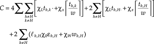
(8.3)

Figure 8.21 Dimensioning results: cost for second and third design methods normalized to the cost of the first method for different values of the cost parameters.
Also in this case, neglecting the integer part to return at the greater integer after achieving the noninteger result, we arrive at a linear expression of the design variables; moreover, as also expected, the hub has a completely particular role in Equation 8.3.
8.4.1.1.4 Comparison between the Design Methods
Since the design methods we have introduced aim at different kinds of network optimization they have to be compared when the cost variables of the network changes. Just to have a feeling of what happens, let us put χx = v χL and χ0 = 3χw = z χL so as to have only two cost parameters: z and v. Increasing z, the cost of the WDM is more and more prevalent, while the contrary happens decreasing z. On the other hand, the ratio between the cost of the node at layer 1 and at layer 2 is regulated by v. Figure 8.21 reports the network cost relative to the base cost obtained with the first method when the second or the third methods are used.
As intuitive, increasing z, the cost of the WDM links is more important and the design with optimized WDM links becomes preferable. This trend is almost independent of v, since the number of ports of LSRs and OXCs have almost the same trend with z.
With high values of v, an LSR port costs much more than an OXC port, and the hub design that reduces the OXC dimensions at the expense of a double passage of each GLSP through an LSR is not convenient. On the contrary, for low values of v sparing in OXC ports is meaningful, since one OXC port costs much more than an LSR port, thus the hub design is convenient.
Since we have done a very simple example, it is not so relevant the fact that in practice, considering long-haul DWDM systems based on EDFA amplifiers; z is slightly greater than one and v is small, perhaps between 0.5 and 0.2. More relevant is the observation that network optimization depends on cost balance and that frequently in the time interval between the planning and optimization of a new network and the end of its deployment, the cost framework is changed. Thus, in real design, it is important to capture qualitative trends that are constant with respect to market evolution to be able to keep the network design updated in all the circumstances.
8.4.1.2 Design for Survivability
In the previous section, we have carried out a basic example of network design without taking into account any survivability strategy. In reality, survivability has to be taken into account. In the case of ASON/GMPLS networks, both protection and restoration can be implemented and each of them can be carried out both at layers 1 and 2. Depending on what solution is chosen for survivability, the impact on the network design changes and network availability has a different value.
Since we are dealing with a simple example to underline the main points of network design, in considering survivability, we will assume to face only fiber cables cuts or DWDM line sites failure.
We will assume that the probability of a cable cut in a given time interval t is constant (does not depends on the absolute time period but only on the interval duration) and for a sufficiently small t can be written as
![]()
(8.4)
In our case, Δt is sufficiently small as far as the failure probability will remain much smaller than one and in this case it can be as long as a few months, since the probability that a single link will be broken in a transport network is generally low.
Naturally, if the number of links in the network is very high, the overall probability that one link breaks in the period can be not negligible. In particular, we can assume as a measure of the network reliability the probability that no service disruption occurs in a fixed time if the service was working at the start of the period. We will call this measure network survivability degree D. In Section 8.5, we will give a more precise definition of the standard parameter used for this kind of evaluations: the network availability.
The survivability degree of a network with NL links without any protection and/or restoration mechanism is

(8.5)
where P(failure, t0) is the probability of a failure in the considered time interval when the network was working at the interval start (instant t0) and it is assumed that the single link failure events are independent and their probabilities pf equal and much smaller than 1.
It is important to note, just for an example, that if the network has 100 links and the probability pf in the network repair time is 2 × 10⁻⁴, the result of (8.5) is D ≈ 0.98, that is clearly unacceptable in front of a normal request of 1 − D = 10−5.
This clarifies the need for a survivability strategy.
8.4.1.2.1 Link 1 + 1 Dedicated Protection
This is the most effective but also the most resource-hungry survivability strategy. Every single link is doubled with another identical link running physically on a different path. This is done by deploying, for example, two identical cables on different sides of a highway or of a railways so that if one is broken, the other is sufficiently far not to be involved in the accident. Every node has a protection switch in front of the receiver and the transmitted signal is doubled and sent both on the working and on the protection path (see Figure 8.22).

Figure 8.22 Block scheme of 1 + 1 link dedicated protection.
If this protection strategy is chosen, the base cost of all the fiber infrastructure is more than doubled (since for each link we have twice the number of amplifiers, DCFs, and so on and moreover we have to add the protection switch card with all the related monitoring), but the network design remains the same. The failure probability of such a protection mechanism adopted is such that within the repair time both the working and the protection links fail.
The probability of two failures on two specific links is, in a first approximation,
Thus the survivability degree can be approximately expressed as
![]()
(8.6)
where P(fail) is given by
![]()
(8.7)
If the network has 100 links and pf in the network, repair time is 2 × 10⁻⁴; the result of is D ≈ 0.999996, a value compliant with values required for D in real networks.
8.4.1.2.2 Optical Channel: 1 + 1 Dedicated Protection
In this case, every GLSP is routed two times in the transport layer on two optical paths such that the links of the working path are never in the same SRLG with any link of the protection path. In our example, we have to connect the following node couples: (2,3), (1,3), (3,4). For each couple of node, two completely disjoined paths are to be found following the desired design criterion.
From the topology, it is quite clear that a design with the hub is impossible in this case due to lack of sufficient topology connectivity. Considering the minimum node cost design, suitable couples of paths are listed in Table 8.5.
Table 8.5 List of Working and Protection Paths for the Minimum Node Cost Design
GLSP Ends |
Working Route |
Protection Route |
(2,3) |
2→3 |
2→4→3 |
(1,3) |
1→4→3 |
1→2→3 |
(3,4) |
3→4 |
3→2→4 |
If dedicated protection is to be implemented, the signal has to be doubled by a splitter after the OXC and sent simultaneously on the working and protection paths. Thus, looking at Table 8.5, two links have to be equipped for protection only (links 1–2 and 2–4) and six more wavelengths are needed.
In a certain number of real situations, the protection paths can be identified as follows:
The working path is routed following the chosen routing criterion.
A new topology is constructed by eliminating all the links traversed by the working path.
The path is routed again using the chosen criterion in this new topology to obtain the protection path.
In the hypothesis of using the OXC switching capacity to double the signals and to feed the working and the protection paths, the cost of the network is given by Equation 8.1 wherein the counts of OXC ports and of links and wavelengths both protection and working paths have to be considered.
In a very first approximation a service disruption occurs if a working path and its protection path both fail during a repair time. Thus probability of failure of a path can be calculated starting from the number of links composing the path. In particular, let us assume to have Np working paths (three in the example) and the same number of protection paths, each composed of Hj hops j = 1 … 2 Np), so that in our example, always considering the first design method, [H] = (1, 2, 1).
The path failure for the j-th path (that can be working if j ≤ Np, otherwise protection) is then

(8.8)
so that a failure that cannot be faced occurs when during a repair time both working path and its protection path fails. The survivability degree, in a first approximation that is valid if the path failure probability is much smaller than one for all the paths, is thus given by

(8.9)
In the example network with 100 links and pf 2 × 10⁻⁴, we will assume a number of routed optical paths equal to 40 with an average length of 5 hops each. With this features D ≈ 0.99996.
8.4.1.2.3 Optical Channel: 1 + 1 Shared Protection
From the routing of protection paths in the example network we are considering, it is evident that some sharing of protection resources can be carried out, paying it with a lower efficiency of the protection mechanism because of losing capacity of facing simultaneous single failures on different paths.
In particular, in our example, in the dedicated protection scheme, two protection wavelengths are routed along the link 2–3. If facing a simultaneous failure of working connections 1 → 3 and 2 → 4 is not a requirement, a single protection wavelength can be equipped on the link 2–3 so that it is used both to protect connection 1–3 and to protect connection 2–4. The OXCs will suitably switch so to create the correct routing of the protection path.
Naturally, if dedicated protection needs only advertising through the control plane, but switches on without any protocol operation, this is not true for shared protection. As a matter of fact, the intermediate OXCs that have to switch to assign the shared protection resources to the right path have to be informed by a control plane protocol of the configuration to implement.
In this case, the network cost is that explained in the previous section, without the wavelengths and OXC ports that now are not needed due to protection resource sharing. A general expression of the survivability degree D is quite difficult to provide for the shared protection, as D depends on the effective sharing of protection resources and then on the topology.
However, a lower bound for D is immediately obtained by assuming as failure probability the probability that two working paths will fail in the repair time plus the probability that a working path and its associated protection both fail during the same repair time.
Thus the lower bound can be approximately expressed as
![]()
(8.10)
where P(fail,1) and P(fail,2) are the failure probabilities for the two failures cases and are given by
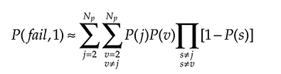
(8.11)

(8.12)
In the example network with 100 links and pf 2 × 10⁻⁴, a number of routed optical paths equal to 40 with an average length of 5 hops each. With these features D ≈ 0.9996. Shared protection can arrive in this example to lose one “9” in D, in front of a relevant sparing in protection resources when the sharing is relevant and thus D is near its lower bound.
8.4.1.2.4 GMPLS Restoration
The extreme form of sparing in survivability resources is GMPLS restoration. When restoration is set up there is no preassignment of survivability resources to specific paths, but a set of resources is assigned to restoration and left unused up to the moment a failure occurs. When a failure occurs, the control plane eliminates the failed link from the topology and reroutes the failed GLSPs using restoration resources.
In general, a complex algorithm is needed to reserve the minimum amount of restoration resources to face the desired set of failures (e.g., all the single link failures), but in the simple example we are dealing with, it is quite clear that if a spare wavelength is installed in links 1–2, 2–3, 1–4, and 3–4, whatever optical channel is involved in a single failure can be rerouted on the spare wavelengths. Thus restoration, in this specific case, to face all single-channel failure, needs 4 spare wavelengths (in each direction) and consequently 16 spare OXC ports.
When a channel is restored using restoration resources, these are occupied; thus, in our example, no other channel can be restored. As in the case of shared protection, in complex situations it is quite difficult to evaluate the exact network survivability degree, but a lower bound can be evaluated.
Such lower bound is obtained by assuming as failure probability the probability that two working paths will fail in the repair time plus the probability that a working path fails besides a single restoration reserved link.
Thus we can write, as in the previous section,
![]()
(8.10)
Where P(fail,1) is given by Equation 8.11 and P(fail,2)
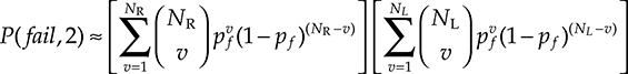
(8.13)
where NR is the number of links dedicated to restoration.
In the example network with 100 links for working paths and 30 links reserved for restoration only and pf 2 × 10⁻⁴ the lower bound is D ≈ 0.99948.
8.4.1.2.5 Comparison of Various Designs for Survivability
We have seen four possible single-layer survivability strategies starting from the more effective and also more expensive in terms of network resources and arriving at the most effective in terms of resources allocation but also less effective in terms of survivability degree. In any case naturally the resulting availability is at least two “9” better than the value of D achieved without any spare resource in the network.
Naturally multilayer survivability strategies can also be implemented, but it is not the scope of this simple example to go so farther and we will return to these more complex solution in a more general analysis later. Now we want to carry out on our simple network an economic comparison between the different strategies taking as a reference the minimum node cost design method.
The survivability degree for the network in Figure 8.20 if the different survivability strategies are used is reported in Table 8.6 if pf = 10−4.
From a network cost point of view, we can take as cost reference the cost of the network designed with the same criterion but without any survivability strategy. The relative cost of the various survivability strategies are reported in Figure 8.23 versus the normalized cost parameters v and z.
Table 8.6 Survivability Degree for the Network in Figure 8.20 if the Different Survivability Strategies Are Used
Survivability Strategy |
Survivability Degree |
Link dedicated 1 + 1 protection |
0.99999996 (seven “9”s) |
Optical channel dedicated 1 + 1 protection |
0.9999998 (six “9”s) |
Optical channel shared protection |
0.9999997 (six “9”s) |
Optical channel restoration |
0.9999996 (six “9”s) |

Figure 8.23 Dimensioning results: cost of survivable networks normalized to the cost of the first method of design without survivability for different values of the cost parameters.
It is evident that the difference in the cost of survivability is great: the most expensive case is 1 + 1 link protection and the dedicated 1 + 1 channel protection. The relationship between the cost of shared protection and the cost of restoration is completely dependent on the particular topology and traffic, thus can be quite different from network to network. In any case, a qualitative idea is given by the network sharing degree, that is, the average number of working path that share a certain protection wavelength on a protection link in the shared channel protection.
It is intuitive that this parameter impacts also the quantity of spare capacity needed for restoration and in general higher the sharing degree, higher the cost advantage that restoration has on shared protection (even if counterexample can be found with a suitable choice of the topology and the traffic). In out example, the sharing degree is 1.3, quite low, thus shared protection and restoration are not so different in cost and in survivability degree. It exist even a value of z above it shared protection is cheaper than restoration. Both are however quite cheaper with respect to dedicated protection.
8.4.1.2.6 Design in Condition of Uncertain Traffic
A last step in the design of our example network before generalizing our considerations to provide design tools that are valid for every network: what happens when the traffic is not known?
If the traffic is completely unknown, no design can be done, different from placing a tentative capacity on each link and see what happen. However generally traffic estimation exists, but it is not sufficiently accurate to allow an optimum design to be realized.
In this case the design has to leverage the statistical description of the traffic fixing a maximum acceptable block probability (that is, the probability that an GLSP setup request has to be rejected) and designing the network to assure a blocking probability at most equal to the maximum acceptable.
We will detail much better this problem dealing with general design methods, for now the discussion about our small example can be considered ended. It allowed us to introduce a set of fundamental concepts for the network design:
The description of multilayer networks in terms of virtual topologies
The balance between grooming and transparent pass-through in multilayer nodes
The possibility to express the network cost as a linear function of the design variables
The necessity of deciding a survivability strategy
A way in which network survivability can be quantified
The different impact on costs of different survivability strategies
Last but not least an idea of how the design can be carried out in conditions of uncertain traffic
8.4.2 Design Based on Optimization Algorithms
The most direct way to generalize the design methods we have used in our example is to set up an optimization algorithm working on a completely general multilayer topology and aimed at optimizing the cost of the network evaluated with a more accurate and general model.
Leveraging on the observation that in our example, neglecting the integer part appearing in the platform cost, the cost function was always linear in the design variables we will target a problem formulation compatible with integer linear programming (ILP), which is a well-known method to model a class of NP-hard problems whose optimization variables are integer [6–9].
8.4.2.1 Optimized Design Hypotheses
The first step to do to develop a general design procedure that can be applied to every topology and traffic request is to define the design problem data. We will assume a few very general hypotheses to restrict the problem and make it solvable.
The infrastructure is completely given; that means that geographical position of Points of Presence of the carrier and of fiber cables are given. Equipment can be installed only in the points of presence, but for in-line amplifier sites of DWDM systems.
We will assume that no OADM branching point exists in DWDM systems.
We will work in terms of nodes topology: the topology in which the physical network nodes are represented by the nodes of the topology graph. A completely equivalent model can be carried out in the so called links topology, where the topology graph has nodes representing the physical network links. An example of corresponding links and node topologies are given in Figure 8.24.

Figure 8.24 Example of (a) node topology and (b) corresponding link topology.
We will image that all the fiber cables are owned by the carrier that is designing the network so that the bare use of a free fiber does not entail a cost and a fiber is always available on each route where a cable is present. However, the model can be generalized without changing the base definitions if the fibers are leased and using a fiber is a cost for itself. Also a possible limitation of fiber availability can be easily introduced without substantially changing the model.
The topology will be meshed at every network layer; design of multiring networks is an important subject, based on different algorithms, and we encourage the interested reader to start the study on multiring networks design from Refs. [10–12].
The layering is also fixed: physical layer is composed by a WDM transport network based on OXCs. We will assume that the OXCs are opaque and that every link between adjacent OXCs has been correctly designed under a transmission point of view so that we need not deal with transmission systems design when designing the network.
The client layer is assumed to be an MPLS layer that interfaces the optical layer via the GMPLS overlay model interface. This means that a node comprising an LSR only cannot exist in the network since in the overlay model, the LRS cannot interface DWDM systems and OXCs directly in other nodes.
The design of optically transparent networks is an important subject that we will consider in Chapter 10. The opaque hypothesis also implies that wavelength continuity is not required in crossing an OXC, since the opaque switching machine also performs wavelength conversion.
In principle, not always an LSR is superimposed on an OXC, and only when it is true, it is possible to communicate between layer 2 and layer 1. Since in practical networks it almost never happens that a node has no local traffic, we will assume that an LSR is always superimposed on an OXC at every node.
Equipment type is already selected when doing network dimensioning at every network layer, thus all the cost parameters are given. In particular, the DWDM layer is composed only of one type of wavelength channel with a given capacity (let us say 10 Gbit/s).
As far as QoS is concerned, we will simplify the situation with respect to a real-istic case and we will assume that all the GLSPs are on the same level as far as the survivability is concerned. Also in this case introducing high priority (that is, protected or restored) and best effort GLSPs simply complicate a bit the model, but does not introduce any new element. Introducing realistic QoS classes on the contrary has quite an impact on the optimization model. Several studies have been done in this direction, see, for example, Refs. [13,14].
We will also assume that a maximum number of GLSPs requests can be done between the same couple of nodes. This is a reasonable limitation, aimed at limiting the number of ports of the network nodes. All the MPLS LSPs will have the same capacity (e.g. 1.2 Gbit/s) that is assumed the unit of capacity of the network. Also this condition can be removed with a slight modification of the optimization algorithm if it is needed.
In principle, an ideal optimization should be carried out by contemporarily assigning both working and survivability resources. We will see that the ILP problem deriving from the multilayer optimization is very complex (precisely NP-hard). Thus, to simplify the solution under a computational point of view, we will design the network in two steps: first assigning the working resources and in a second phase the survivability ones.
The decision of performing a two-step dimensioning, first working capacity and then protection or restoration, deserves some comments. Several studies in literature demonstrate that final network cost is quite near the optimum when proceeding in this way [6], while the computational complexity is sensibly reduced. Besides in terms of computation complexity, this approach has the practical advantage to allow simulation of different survivability mechanisms by designing the working part of the network only once.
We will exploit this feature in the last part of the chapter, when we will compare different survivability strategies maintaining the same traffic and network. These hypotheses are a sufficient base to lay the foundation for a general network design method based on ILP. In order to do that we have to built a general description of the network that is suitable for the scope.
8.4.2.2 Network Model for ILP
In a multilayer network model, a set of topology and traffic variables can be defined at the same way at infrastructure layer (layer 0 in our model), at the optical layer (layer 1) and at the MPLS layer (layer 2). We will call them with the same symbol with a suitable prefix. The layer prefix will be written on the left of the symbol, so that it is not confused with indices representing elements of a matrix.
For example, the number of nodes will be indicated with 0N if we are considering the infrastructure layer, with 1N if we are considering the optical layer, and 2N if we are dealing with the MPLS layer. Naturally variables at different layers are related, in this case 0N ≥ 1N = 2N.
The topology will be described by two matrixes: the adjacency matrix [sA], whose dimensions are sN × sN (s = 0, 1, 2), and the link matrix [L], which exists only at the physical layer. The element sαij of the adjacency matrix is 1 if at the s th layer the nodes i and j are connected via a layer direct connection, otherwise it is zero. The element ℓij of the link matrix contains the length of the physical cable connecting nodes i and j at layer 0 if this cable exists, otherwise it is zero.
The traffic is defined through a traffic matrix [T] of dimension 2N × 2N that contains the request of traffic in terms of LSPs to route in the MPLS layer, its element τij represents in particular the number of LSPs to route between node i and node j of the MPLS layer (layer 2).
If the traffic forecast is not sufficiently reliable, the matrix [T] has to be derived from the traffic statistics with a statistical model. For the moment we will assume that [T] is given, we will analyze in the next section a draft method to manage traffic uncertainly.
We will call
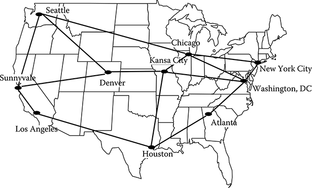
Figure 8.25 Reduced version of the North American network used for the examples of this chapter. The link length is assumed equal to the highway distance between the corresponding cities.
The maximum number TM of LSPs to be routed between a couple of nodes is given by
However, in the network we have chosen as an example and in general in any network, it is possible to set a maximum number of hops per LSP and it is quite small (generally much smaller than N). For example, optimizing with random traffic the network of Figure 8.25 the maximum number of hops results to be 3 at optical layer and 2 at the MPLS layer. As a matter of fact, more hops generally means longer transmission and more costly DWDM.
Let us assume that H is the maximum number of elements different from zero in one slice of [sR] obtained by srijkdv varying k and d and maintaining constant the other indices. Let us also assume that it is the same for all the layers. Due to the meaning of the elements of [sR], H results to be the maximum number of hops of a GLSP on layer s.
The matrixes [sR] have a maximum number of sN2H2 elements different from zero, which in the previous example is 900 for s = 1 and 400 for s = 2.
Moreover, as we will see in detail, the property that all GLSP are bidirectional can be used to further reduce the number of variables, arriving to 450 for s = 1 and 200 for s = 2 out of a total of 30,000. Thus, if it is needed to compact the representation of the matrixes [sR], it is possible to adopt a sparse matrix representation. This can be also beneficial to speed up searches in the matrix and thus calculation.
One way to do that is to represent [sR] through a 2N × 2N × M pointers matrix and to append to each pointer a list of the only nonzero elements with the first two and the last indexes equal to the indexes of the pointer. The records of the list will be H2 and each of them will contain the third and the fourth indexes of the nonzero element of [sR].
This representation has also an important physical meaning that helps in implementing the algorithm. The first two indices are the two ends of an LSP while the last index is the order number of that LSP among all those with the same ends. Thus every pointer represents an LSP and it points to records representing the links traversed at layer s by that LSP.
The computation complexity of the final algorithm is a different issue, which is also triggered by the great number of design variables and we will discuss it at the end of the section. Returning to the definition of the routing matrixes, it is relevant to underline that if an LSP of the MPLS layer is routed through the hth node of the optical layer while it is merged in an optical channel, but it is not sent to the local LSR, we will have 1rijkhv = 1, but 2rijkhv = 0 since it does not travel through the node in the MPLS layer, but only in the optical layer. This shows as in the multilayer representation of routing the grooming is automatically comprised.
The matrix [Λ] is a 1N × 1N matrix and λij represents the number of wavelength connecting node i with node j to route the LSPs. The wavelength channels connecting OXCs and transporting LSPs that travel only at the optical layer without being extracted by the wavelength up to their destination can be considered GLSPs in the optical layer.
The elements of the matrixes [sR], [Λ] are the design parameters and the solution of any optimized design has to provide values for these elements. However, this determines also the number of variables of our ILP problem and from this point of view, this is clearly quite a big number. Thus frequently simplifications are introduced to decrease the number of variables. We will discuss a few ways to simplify the problem when we will have a complete algorithm formulation.
Considering the cost model, we will use a generalization of what we have assumed in our example in the last section. Every equipment has a cost constituted by two terms: a platform and an interfaces term.
DWDM systems cost is given by
 where l is the system length and w is the number of wavelengths, while χw0 and χw1 are constants typical of the system. Mw is the number of wavelengths supported by a single system and ⌈x⌉ indicates the smaller integer greater than x. We will also call W the normalized capacity of one wavelength in term of LSPs (maintaining for definition equal to one the capacity of each LSP).
The cost of OXC is given by
 where q is the number of bidirectional line ports of the OXC, Mq is the number of bidirectional line ports supported by a single platform unit (e.g., a single rack), and ⌈x⌉ indicates the smaller integer greater than x. The parameters χx0 and χx1 are normalized cost constants typical of the OXC.
The cost of LSR is given by
 where u is the number of bidirectional line ports of the LSR and Mu is the number of bidirectional line ports supported by a single platform unit (e.g., a single rack). The parameters χL0 and χL1 are constants typical of the LSR.
The number uj of bidirectional ports of the jth LSR can be calculated as the sum of the locally generated LSPs plus the number of transit LSPs that are sent to the LSR to perform grooming optimization.
Thus

(8.14)
Similarly, the number qj of bidirectional ports of the jth OXC is given by

(8.15)
Finally, neglecting the ⌈x⌉ operator to maintain the linearity of the cost function, the ILP target function writes

(8.16)
The target function is linear in the design variables as desired. In this condition the resulting problem is an ILP problem if suitable constraints are set. Arriving at an ILP requires elimination from the cost function the lower integer part to the addenda representing the platform cost of the equipment. This is not a small approximation and it is worth a comment.
Generally, deploying a new DWDM system or a new OXC is an expensive operation with respect to adding a new wavelength to an existing DWDM or a new card to an existing OXC. This is exactly due to the integer part operation that we have neglected in the cost function: that operator represents the fact that the whole platform cost is paid when the first equipment card is installed.
Thus, while in practice the deployment of a new system is always avoided if possible, in our problem, this would not be true, since the first card will have the same cost of all the others. This approximation is important mainly in the case of DWDM systems whose platform has a high cost due to amplifiers and other line equipment.
In specific cases, this approximation can cause the solution to be far from optimum. This situation is detected when there are a lot of DWDM systems or OXCs and LSRs with a very low number of wavelengths or interfaces, only one in the limit case.
In this case, it can be beneficial to create a postprocessing routine that tries to eliminate these systems by rerouting the wavelengths on already existing equipment and verifies if the cost of the network can be lowered in this way. We do not detail how such post-processing can be implemented, technical literature on such heuristics is very rich, and the interested reader can start to approach the problem from [15]. To obtain the results presented in this chapter, no postprocessing is used since looking at the obtained solutions shows that the platform approximation is never so important to change the results significantly.
Considering the constraints, we have to maintain them linear if we want to formulate an ILP problem. The first set of conditions is the flow continuity across the nodes at every layer. This means that at every layer the traffic entering the node from client and line ports has to balance the traffic exiting from client and line port. Looking at the LSR, the continuity, coinciding with the bidirectional nature of the LSR, can be written as
![]()
(8.17)
![]()
(8.18)
It is important to note that even if (8.17) and (8.18) are constraints, they can be imposed directly on the routing matrix with the effect of reducing the independent variables and decreasing the overall complexity. This is particularly easy if the sparse representation is used for the routing matrix, where LSPs appear explicitly. In this case, only the variables representing an LSP in one direction have to be considered, so halving number of elements of the pointers matrix.
While looking at the OXC we have two continuities, one in terms of wavelengths and one in terms of LSPs. In terms of wavelengths we can write
![]()
(8.19)
which means that the wavelength matrix is symmetric.
In terms of LSPs, the bidirectional condition is written as
![]()
(8.20)
![]()
(8.21)
Last but not least the continuity at the layers’ boundary has to be set. Remembering that an LSR is always present where there is an OXC, we can say that the LSPs traversing the LSR (that is, passed from layer 1 to layer 2 in the nodes) will be in general a subset of the LSR traversing the OXC. This subset has to coincide with the set of LSPs carried by a certain number of wavelengths.
Mathematically this condition is expressed as
![]()
(8.22)
Moreover, the number of LSPs terminated in a node has to coincide with the corresponding entry of the traffic matrix, thus
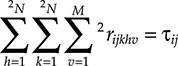
(8.23)

(8.24)
After the bidirectionality, it is needed to assure that the number of wavelengths deployed on each link is sufficient to support the traffic routed along that link and to assign the LSPs to the wavelengths so that passing a set of LSPs between the layers at a certain node coincides with the termination of a certain number of wavelengths in that node. This con-straint requires to introduce the number of wavelengths terminated in a node and the number of wavelengths that bypass the node without termination.
We will call [Ω] ≡ {ω kh} the 1N × 1N matrix containing the wavelengths bypassing node k when arriving from link h-k. The requirement of a certain wavelength number is written as

(8.25)
while the condition on the wavelength termination, utilizing the fact that the locally dropped LSPs are the same both on layer 1 and on layer 2, can be written as

(8.26)
and finally
![]()
(8.27)
where W is the maximum number of MPLS LSPs that can be multiplexed into a wavelength.
After the constraints on bidirectionality and capacity, we have to impose the GLSPs continuity through the network. This means two things:
If the routing matrix tells that a certain GLSPs travels at layer s from node h to node k with one hop, these nodes have to be contiguous in their own layer, which means that sαhk have to be equal to 1.
Successive hops have also to be contiguous, that is, the GLSP can go from node h to node k and then from node k to node j, but not from node j to node v, since after the previous step it was in node k.
First, let us introduce the maximum number of hops sD allowed to the GLSP in the network at layer s (it can be sN in the extreme case).
The first condition involves obviously the adjacency matrix at the given level, and is written as
![]()
(8.28)
which says that if 1rijkhv = 1, implying that the vth path routed through the nodes j and i passes through the link h-k, thus the link h-k has to exist.
In order to express the second condition we can notice that a matrix [srijkhv] where k and h are the running indexes while the other are fixed represents the path of a GLSP that, by definition, has no loops. Thus only one element per line and one element per column can be different from zero, which is the same as saying that the path enters into the hth node of the topology only one time and exits from it only one time.
The previous conditions can be written in term of constrain compatible with ILP as
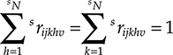
(8.29)
If the condition (8.29) is a constrain of the problem, we are sure that only one element is different from zero among the elements of a column and of a row.
The last step is to express the fact that the path of an GLSP has to be made by adjacent links, that is, the set of nonzero elements srijkhv. with i, j, v fixed has to be constituted by concatenated elements like (srijihv, srijhkv, srijkjv).
This condition can be expressed by the use of the adjacency matrix. From the nodes adjacency matrix, a links adjacency matrix [sB] can be easily derived, whose elements sβijk are equal to one only if the two adjacent links i, j, and j, k both exist. In particular, it is immediately seen that sβijk = sαi,j sαj,k.
Thus the condition we are searching is written as
![]()
(8.30)
The meaning of this constraint is the following. Starting from srijikv, which are the unique nonzero elements with the first and third index equal to i, the second equal to j and the fifth equal to v, a chain of elements of [sR] can be constructed by adding to each element the following element having the same first, second, and fifth index and the fourth index moved at the third place.
These last conditions also define a unique nonzero element, so that, if a valid path has been found between i and j, it can be constructed in this way. This also implies that both srijhkv, and sr ijkxv,, representing adjacent links of the path, are equal to 1. From this property derives the fact that Equation 8.26 is satisfied.
A similar continuity constraint has to be written across a node for the wavelengths that are not passed to the upper layer by the OXC. In particular, the number of passing through wavelengths entering the OXC has to be equal to the number of passing through wavelengths exiting the OXC.
This condition however is automatically satisfied by the coexistence of the constrain (8.18) and by the property ωkh = ωhk deriving from the bidirectional nature of the GMPLS GLSPs. The equations we have derived up to now are sufficient to dimension the network with optimized resources to sustain the traffic, but without any survivability strategy.
In order to add survivability resources a further dimensioning step has to be done. This step is sensibly different if protection or restoration is used. We will limit ourselves to describe the algorithms that can be used in this second step, leaving to the reader the construction of the optimization equations.
8.4.2.2.1 Optical 1 + 1 or 1:1 Link Protection
This is the simplest case; every optical link is protected through a similar link connecting the same nodes, but running on a different path (e.g., on the opposite sides of an highway or of a railway). The 1:1 protection differs from the 1 + 1 only because in the first case low-priority traffic can be routed on the protection capacity when it is not used while in the second case the working signal is sent also on the protection path to render recovery against failure the fastest possible.
In this case the transmission capacity of the links and the switching capacity of the nodes at the optical layer increments by 100%. The only attention to be paid is not to duplicate uselessly the OXC platforms using when possible for protection platform-free space that is present in the platforms already installed.
8.4.2.2.2 Optical 1 + 1 or 1:1 GLSP Protection
At the optical layer, the GLSPs are the wavelength paths. A wavelength path starts when a set of LSPs with the same destination are aggregated by an LSR in a wavelength and sent to the collocated OXC and terminates when the wavelength is extracted by the optical layer to be delivered to the destination LSR.
There is no data structure in our network model that represents directly the optical GLSPs, thus they have to be derived from the information we have. In particular, the fol-lowing criterion can be used.
Every LSP is routed through the network in a known way so that it is possible to divide the LSPs into groups so that each group is formed by LSPs starting for node k, traveling through the same set of nodes on the same links and ends with the node h. They can be either LSPs that really start for a layer three request in k and end in h or LSPs that are injected in the optical layer in k or in h or both after grooming at the MPLS layer.
The extreme case is that of an optical GLSP that starts in node h from the aggregation of LSPs collected by other optical GLSPs via grooming at layer two and ends in node k where the LSPs are distributed among other optical GLSPs to be transported to destination.
Once the groups are constructed, every group corresponds to one or more optical GLSPs, depending upon the group cardinality and on the number of LSPs a wavelength can accommodate. Once a map of the optical GLSPs is created, a protection path is completely disjoined from the working path has to be preprovisioned for each of them.
To do that three matrixes have to be defined:
The optical traffic matrix [Q] whose elements qhk represents all the layer 1 GLSPs (the wavelength paths previously calculated) connecting node h with node k.
The working routes matrix [ψ] whose generic element ψijhkv is equal to one if the vth working wavelength path starting from node i and terminating in node j transits through the link h-k.
The protection routes matrix [Ф] whose generic element ϕijhkv is equal to one if the vth protection wavelength path starting from node i and terminating in node j transits through the link h-k.
The first two matrixes are easily derived from the solution of the working optimization problem, the third matrix elements are the parameters of a new single layer ILP problem where the traffic [Q] is routed in the optical topology and the condition that working and protection paths have to be disjoined is guaranteed imposing the condition ψijhkv ϕijhkv=0.
8.4.2.2.3 Optical Shared Protection
In this case, before going on with the design of the protection, a data structure has to be constructed where the working optical GLSPs are divided into sets so that the GLSPs of one set are routed on paths completely disjoined by the GLSPs of the other set.
After that, when performing the optimization, for every link assigned for protection, the sets of the working GLSPs protected through that link are determined and tagged on the link. To assign the protection capacity for a certain working GLSPs, let us say the GLSP with ID equal to 123 belonging to the fourth group, all the protection links that are not tagged with the fourth group are considered available capacity to route the protection GLSP.
8.4.2.2.4 MPLS 1 + 1 or 1:1 Protection
In this case, for each MPLS LSP, a protection path has to be preprovisioned that is com-pletely disjoined from the working path. The optimization is carried out using the same approach already used for 1+1 optical protection with a further step: the possibility that new wavelengths have to be introduced due to the need of routing the protection LSPs. Naturally before adding resources to the network the unused resources already present have to be exploited. A new wavelength is introduced on a certain optical link only if no wavelength exists where the working LSP is not multiplexed and with enough free capacity to host the protection LSP.
8.4.2.2.5 MPLS Shared Protection
In this case, in analogy to what was done for the shared optical protection, before going on with the design of the protection, a data structure has to be constructed where the work-ing LSPs are divided into sets so that the LSPs of one set are routed on paths completely disjoined by the LSPs of the other set.
After that, when performing the optimization for every link assigned for protection, the sets of the working LSPs protecting through that link are determined and tagged on the link. To assign the protection capacity for certain working LSPs, not only the free capacity left by the routing of the working traffic is considered available, but also all that link that has been introduced to route protection paths and that are not tagged with the group to which the link under analysis belongs.
8.4.2.2.6 Restoration at Optical Layer
In case of use of restoration at the optical layer, the OXC manages the restoration procedure in such a way that the MPLS layer does not detect the failure if possible. Different types of restoration exists, depending on when the restoration resources are assigned to the LSPs affected by a certain failure event. Among them we will consider three cases:
Type 1. Restoration resources are reserved and the connection is set up after the failure. In other words, the optical GLSPs affected by the failure are rerouted in the network as if they were new requests of connection delivered directly at the optical layer. If new connection requests arrive during the restoring phase, they go in competition with the GLSPs to be restored.
Type 2. Reservation is made before the failure (but without a links with a specific failure event) and the path setup is performed after the failure. If new connection requests arrive during the restoring phase, no competition with the GLSPs to be restored happens due to the assignment of the restoration resources to survivabil-ity only.
Type 3. Resources are reserved to survivability and a certain number of restoration paths are set-up. When a failure occurs, the affected paths are rerouted using the prepared restoration paths. This is the most rapid restoration, based on the setup of a certain number of prereserved paths. Naturally it is also the most resource-hungry restoration technique.
When restoration is used, an effective way to operate is similar to that of shared protection, but for the fact that in Type 1 restoration even the parts of the working GLSP that are not affected by failure are considered available as restoration paths.
In order to take into account this strategy, the following algorithm can be used to design the restoration capacity: for each link in the topology graph, the link is elimi-nated and the GLSPs involved are determined. These GLSPs constitute a capacity to be routed through the network without the failed link. This can be done with an ILP algorithm to optimize the resources use. Generally the cost of the restoration part of the network has to be recalculated since the final solution will not coincide with one of the partial solutions.
From a complexity point of view, it could seem that restoration design is much more complex than working capacity assignment, due to the fact that one ILP optimization is required for each network link. This is generally not true due to two facts: the first is that only the optical layer is involved in the routing, grooming is not permitted during this type of restoration to avoid multilevel signaling. Moreover, only a few elements of the traffic matrix are different from zero, contributing to lower computation complexity.
8.4.2.2.7 Restoration at GMPLS Layer
The procedure is quite similar to that carried out for restoration in the optical layer, with the same three restoration types. The difference is that now there are the MPLS LSPs to be restored, so that we have to face a two-layer optimization. This allows grooming to be used also when designing restoration resources generally with a better result with respect to the same restoration strategy adopted at the optical layer.
On the other hand, the complexity of the whole design algorithm is quite higher.
8.4.2.2.8 Final Comment on Survivability Resources Design
We have presented a set of methods to design survivability resources independently from working resources. This is for sure a suboptimum procedure, but as we have seen has a certain number of advantages. In any case, several optimization methods have been proposed in literature that does not divide the planning of working and survivability capacity. They are strictly related to a specific survivability method, but in principle, provide an optimum solution to the planning problem.
Naturally, the complexity of such a design method is higher with respect to what we have used here and generally some approximation is in any case used to make the problem solvable. For a discussion on different joined optimization methods, see Refs. [6,8,9].
8.4.2.3 ILP Design Complexity
The ILP optimization model we have presented in the last section is very explicit in representing the capacity routed on every link, which is useful in those cases in which DWDM links have to be designed after the network general optimization.
Other model exists that are a bit less complex from a computational point of view [16–18], however, whatever model is defined, the optimization of a multilayer mesh network is an NP hard problem, which means that the problem nature implies an exponential complexity increase with the key scale variable, which in our case is the number of nodes. Thus it is important to understand how the computation time can be shortened and what does it mean in terms of accuracy of the found solution. A very good analysis on this point is reported in Ref. [6] and we encourage the reader interested to detailed results on specific examples to start from this reference. Here we will cite and justify intuitively a few techniques for ILP complexity reduction without reporting a detailed quantitative analysis.
The first observation is that ILP goes uniformly toward the optimum solution, thus there is a relevant part of the time used by the algorithm to refine an already good solution. There is a measure of how much the configuration found in an intermediate state is far from the final optimization, which is the so-called solution optimality gap to be evaluated comparing the fully optimized solution with the intermediate one and measuring the cost difference in percentage with respect to the optimum cost.
It has been demonstrated in Ref. [6] a quite general result regarding algorithms like this: if an optimality gap of the order of 3% is accepted the computation time can be significantly shortened and even quite large networks can be analyzed.
In our case, trying to find a full optimal solution in the case of the network with 15 nodes and 25 links with a dense traffic matrix requires a vector computer or a very long time. However, in few hours of working on a well-equipped workstation a solution with a cost within 3% from the optimum can be obtained.
In practice, of course, the optimum solution is not known and the optimality gap cannot be evaluated exactly. However, observing the solution evolution for different running times it is not difficult to estimate the order of magnitude of the solution refinement versus the running time.
Even accepting a certain optimality gap, networks with a number of nodes in the order of 11–13 depending on the traffic matrix and the number of links are the limit for a reasonable execution time. If greater networks have to be analyzed, some more important simplification has to be done.
We can divide the possible simplifications in two classes: physical simplifications related to the particular nature of the problem at hand and mathematical simplifications, which is the mathematical approximation of the original ILP problem that can be applied to all the networks.
8.4.2.3.1 Physical Approximations of the ILP problem
The most important class of simplifications are those aimed at reducing the number of design variables. Generally such simplifications work very well on certain types of network and traffic while they give a poor performance in some specific cases. Now we report a list of possible simplifications that has been successfully used to design large networks, but only direct experience can achieve complete confidence when used on a generic topology.
A first possible simplification is to decouple the design of the MPLS layer and of the optical layer. In this case, two different ILP problems result that are both quite simpler with respect to the joined design problem.
This approach is very effective when grooming has not to be used intensively to increase the effective utilization of the optical channels. In the extreme case in which no grooming is used and MPLS layer and optical layer have separated survivability mechanisms, it is exact. Unfortunately, this is not the generic situation and in real networks excluding grooming brings to a suboptimal design. Naturally smaller the W, more difficult an effective grooming, more performing the method of disjoined design.
Another important simplification is possible when the network is divided into zones and only a few LSRs are routed through different zones. In this case, the problem can be divided into a different problem for each zone and a global prob-lem only for the interzone LSRs.
The single-zone problem can be solved exactly being relative to a network with much less nodes, while if the interzone GLSPs are really a small quantity of the traffic, they can routed through a suboptimum algorithm without affecting greatly the final network cost.
If W is small (that is, the LSR are high speed and a small number of that fit into a wavelength) and the network is poorly connected, further simplification can be achieved assuming that all the paths having the same extremes are routed through the same route. In this case, the routing matrix loses the last dimension, since all the LSRs are routed together. This decreases the number of elements of the routing matrix by a factor M, so simplifying the resulting computation.
If W is great and a large number of GLSPs are routed toward each couple of nodes (that is, the traffic matrix elements are large), the problem can be simplified by creating sets of GLSPs and routing them together.
8.4.2.3.2 Mathematical Approximations of the ILP problem
Since it is well known that an ILP problem can be very hard to solve, several mathemati-cal studies have been developed to analyze possible approximations of the problem that reduces its complexity [19,20].
A simple method to obtain an upper-bound and a lower-bound to the solution of the ILP problem is to use the so-called relaxation method. This method simply consists in eliminating the condition that the variables have to be integer, substituting them with real variables. In the particular case in which there is a variable that can be zero or one, this is substituted with a real variable in between zero and one.
The first case happens in our model, for example, for the number of wavelengths in a link and the second for the elements of the matrix [sR].
With these substitutions, the problem becomes a linear programming problem, whose complexity is polynomial, thus solvable also in high-dimensional cases. At the end, the optimum variables will not be integer in general, but the optimum of the LP problem will be a lower bound of the real problem solution; this lower bound is called LP-relaxation bound [20].
In order to derive an upper bound of the solution, the following algorithm can be used:
Construct a problem-acceptable solution by rounding the LP optimum variables to the upper or lower integer as suited.
Substitute these variables into the cost function to obtain the cost relative to the constructed network design.
The obtained cost is an upper bound of the solution of the ILP problem.
The first step of the algorithm is generally not unique and, if several possible networks can be designed rounding to integer value the LP solution, the tighter upper bound is rep-resented by the smaller cost corresponding to one of such networks. This upper bound is called rounding bound [20].
If the upper-bound and the lower bound are sufficiently near, the rounded variables constitute a good approximation of the effective ILP optimum solution. These simplifica-tion methods can make solvable a problem that is not solvable searching an exact solution, but the general nature of NP hard problem remains. This is why, in order to analyze large networks or to analyze a large number of alternatives, completely different design methods have been introduced based on heuristic approaches. These methods provide suboptimum solutions, but are much less complex than ILP optimization.
8.4.2.4 Design in Unknown Traffic Conditions
The design method we have detailed up to now relies on the fact that a reliable prediction of the traffic to be routed in a considered period of time (e.g., between two major network upgrades) is well known and that this traffic is constituted by connections that will last up to the end of the considered period.
In this case, the network design does not depend on the order in which the connections are opened, since the traffic matrix is available from the beginning. This condition is called deterministic static traffic.
The traffic model can be altered essentially in two ways:
Substituting the absolute knowledge of the traffic to be routed in the network with a partial knowledge of the traffic matrix; for example, the element of the matrix can be known only with a great approximation (like 5 < τij < 8) or they can be random variables with a known statistical description. In this case the design is performed in unknown traffic conditions.
Instead to be semipermanent, the connections are setup and tear-down several times in the considered observation period on the ground of some statistics. In this case the network is designed under dynamic traffic conditions.
GMPLS sets up semipermanent connections in the transport and MPLS layers, thus dimensioning in conditions of dynamic traffic does not occurs in the bottom layers of the network. On the contrary, if the dimensioning was performed for a TCP/IP network, since TCP set-up and tear down continuously connections design in dynamic conditions would be needed.
On the other hand, the consolidation of competition among carriers and in general the uncertainty on the penetration of new services renders the knowledge of the traffic matrix less and less precise so that dimensioning is often performed in conditions of unknown traffic.
In order to use a dimensioning algorithm in these conditions, it is needed to set up a method to manage the unknown traffic condition. The problem is widely studied in literature and in general we would like to evidence three possible methods [21]:
A priori adjustment
A posteriori adjustment
Probabilistic approach
In the first two methods, the idea is simply to use a safety margin to face possible fluctuations of the traffic matrix. This safety margin reflects at the end in an overdeployment of network resources with respect to the optimum solution dictated by the average traffic matrix. The difference between the two methods is that in the first the average traffic matrix is augmented by the safety margin and then the optimization is carried out as usual.
In the second method all the optimization is carried out on the ground of the average traffic and at the end more resources are deployed with respect to the optimization output. The key issue in both these methods is how to choose the safety margin to be sure to reduce suitably the network rejection probability (that is, the probability a connection request is rejected by the network) while containing the deployment cost.
A discussion based on statistical approach is reported in Ref. [21] where it is demonstrated that it is possible to select an optimum safety margin starting from hypothesis on the statistical distribution of the traffic both in a priori and in a posteriori adjustment. However, even when the margin is chosen in this way, in particular cases, its use leads to excessive overdeployment in some areas of the network where in other areas resource shortage could still happen for modest fluctuations of the traffic variables. Sometimes the problem is solved considering different safety margins in different zones of the network, but other times this gives no advantage.
In any case, after the design of the network using the safety margin–driven overdeployment, simulations have to be generally performed to verify the effectiveness of the design in reducing the rejection probability.
Better results are achieved via the probabilistic method, which uses directly the knowledge of the traffic statistic distribution.
The easier case is that of uniform traffic variation.
In this case the random traffic matrix [T] can be written as follows:
![]()
(8.31)
where
[T0] is the average traffic matrix.
x is a random variable with average equal to one and known probability distribution
In this case, the problem can be formulated as follows: the network has to be designed so that the probability that a connection request is rejected is smaller than a certain limit, called PR.
The solution is straightforward once the design tool is available. Calling p(x) the probability density of the variable x, it is possible to find a value x0 so that

(8.32)
If the network is dimensioned for the traffic matrix [T] = x0[T0], the rejection probability is surely smaller or equal to PR.
The situation gets more complex if the traffic matrix depends on more than one random variable, but in line of principle the solution method is the same. Let us assume that [X] is a random matrix, with 2N ≤ V ≤ 2N2 nonzero elements, and whose average is the identity matrix [I]. Let also assume to know the joined probability density functions of the V random variables that are elements of [X], called p(x1, x2, …, xV).
If the traffic matrix can be written as [T] = [X] [T0], the method used for the single random variable can be directly generalized. Naturally it is not easy to derive the model of the traffic matrix and its distribution so that, in the absence of other information, a Gaussian model is often adopted. It is possible to imagine more complex models for the random nature of the traffic, for example, based on Markov chains [21]. In this case, the design gets more complex and we direct the reader to the relevant bibliography for a study of the problem.
8.4.3 Routing Policies–Based Design
As we have seen, ILP-based optimization algorithms are quite computationally complex, representing in reality, a particular formulation of an NP hard problem. If they are largely used for dimensioning of networks, it is not possible to adopt them when network dimensioning is only a step of a complex procedure, for example, of a comparison between different network architectures or the study of the network sensitivity to a set of design variables.
In this case, it could be necessary to repeat the dimensioning hundreds of times, which is quite hard using an ILP algorithm if the network is not particularly simple. Other times it is needed to have a first impression of the network deployment with a fast calculation, without resorting to the complexity of an ILP program. A plethora of heuristic network design algorithms have been proposed to be used in these cases, much less computationally hard than the ILP optimization.
A class of design algorithms based on suboptimum design methods is those of the routing-based design. These algorithms are inspired by the automatic configuration of the network and work as follows:
A traffic matrix is individuated either through forecast of through statistical elaboration.
A routing algorithm is also fixed for working capacity at all layers.
Starting from the upper layer, connections are routed assuming the availability of infinite capacity in the network.
At the end of the routing, the nodes and the links are inspected and the equipment required to sustain the performed routing is deployed.
Every time that the dimensioning depends on the order in which the paths are routed, the dimensioning is performed in several cases and the cheaper solution is selected. Moreover the algorithm can be easily generalized to include design of survivability capacity both in cases of protection and restoration.
For example, in case of 1 + 1 optical layer protection, the protection capacity is routed after the working one. In particular, the optical path protecting a link (i,j) is routed in the optical layer virtual topology where the link (i,j) has been eliminated and this procedure is repeated for all the links. Once the protection capacity has been provisioned it is considered occupied exactly like the working one in the successive routing operations, to reflect the 1 + 1 protection.
On the other hand, if shared protection has to be planned, the algorithm is similar, but the protection capacity is considered free for use in successive routing of protection optical paths with a procedure similar to that adopted for shared protection in the section dealing with ILP.
A great number of routing policies has been proposed as basis of the network design. We will introduce and comment few of them [15] limiting the comment to the design of the working capacity and of the optical layer only. Extension to a multilayer network is immediate.
8.4.3.1 OSPF Protocol
This is the simpler choice, suggested by the fact that is one of the most diffused routing protocols. Moreover, it is possible to shape the working of the protocol by tagging the network links with a suitable tag and, in case, tagging also the crossing through a node.
The algorithm corresponding to pure OSPF for the routing, as it is generally used in dimensioning tools, remembering that in this case infinite resources are assumed, can be described as follows:
Evaluate the shortest path between source and destination with the given graph metrics.
If on every link there is an incomplete DWDM system with available wavelengths, route the GLSP and go to END.
If there is no wavelength available on one or more links, route the GLSP on the shortest path by opening new DWDM systems where needed.
END
The operation of opening new DWDM systems is generally an expensive operation since it requires the deployment of new equipment in the central office and the deployment in the field of optical amplifier places.
Thus sometimes effort is paid to avoid the aperture of a new DWDM system by exploring the possibility of routing the new GLSP on a second shortest path. In this case the algorithm is the following (we will call it M-OSPF: Modified OSPF):
Evaluate the shortest path between source and destination with the given graph metrics.
If on every link there is an incomplete DWDM system with available wavelengths, route the GLSP and go to END.
If there is no wavelength with sufficiently capacity available on one or more links, eliminate those links from the topology.
Find the shortest path in the new topology.
If on every link there is an incomplete DWDM system with available wavelengths, route the GLSP and go to END.
Return to the original topology and to the original shortest path. • Add a new DWDM system when needed and route the GLSP.
END
Naturally this is only one of the possible flavors that OSPF like algorithms can have when used in network design tools. For example, we have listed a version that opens a new DWDM if the second shortest path is also unavailable, but this is not needed. It would be possible to look for the third shortest path and so on. Finally, in this paragraph we have considered explicitly the cost of the links, but the cost of the nodes can be added using the same criterion.
8.4.3.2 Constrained Routing
A different type of routing can be applied when designing a network, more oriented to limit the overall network cost. This is the cost constrained routing whose algorithm can be described as follows:
Set an order for the GLSP setup requests.
For each GLSP, find all the paths connecting source and destination.
With an opportune cost model compute the incremental cost related the possibility of routing the new GLSP on every possible route.
Among the considered paths chose that with the minimum incremental cost.
END
Several routing algorithms can be devised introducing different kind of constrains, for example, on the QoS, on the capacity and so on. A class of interesting constrains are the so called dynamic once. A routing constraint is called dynamic when the tags that are put on the links and drive the constrained routing are not constant but change while the situation of the network evolves.
Naturally also in this case an order in which the setup of the GLSP is request has to be fixed. A classical example is constituted by the CAPEX related to the routing of a new wavelength on a certain link. This is generally constant, but when the routing of the wave-length implies the deployment of a new DWDM system, then it becomes very high so limiting as much as possible the opening of new DWDM systems.
Another typical application of dynamic constrains is possible when the number of fibers connecting the network nodes are not unlimited, for example, since the carrier is leasing them, and the bare use of a fiber has its own cost. In this case the cost of using a link for a new wavelength depends on the link length, on the number of fibers available along the link and on the leasing price if applicable. In this condition a dynamic link cost tag is very effective in performing a correct network optimization.
The design methods based on routing strategies are only one of the classes of heuristic algorithms that has been devised to design GMPLS networks. A more complete analysis can be done starting from the following biographies [22–24].
8.4.3.3 Comparison among the Considered Algorithms
In comparing the different heuristics we have introduced, we will take as a reference the results obtained using the ILP optimization.
The comparison is based on sets of 10 random networks designed to cover an approxi-mately square area of the dimension of Italy for all the considered values of the number of nodes. All the considered networks have a connectivity (average number of disjoined path between couples of nodes) around 2.2 and the design does not include any survivability mechanism.
The traffic matrix is uniform and composed of three GLSPs between each couple of OXC. When the order of the connection request is required the dimensioning is repeated in 10 random orders and the lower cost is accepted. The comparison result is reported in Figure 8.26. All costs are normalized with respect to the optimized cost obtained with the ILP.
The first observation is that there is a good performance of the routing-based algorithms, the cost does not change more that 20% from the value obtained from ILP. The reason essentially has to be found in two characteristics of the considered networks:

Figure 8.26 Comparison among routing based design based on a set of 10 random network for all the considered values of the number of nodes. All the considered networks have a connectivity around 2.2 and the design do not include any survivability mechanism. All costs are normalized with respect to the optimized cost obtained with the ILP.
connectivity and geographic extension. The connectivity is low, generally two paths between any couple of node with a few exceptions, thus a smart optimization algorithm cannot do much better than a simple OSPF having a little number of alternatives. Moreover the number of nodes is also low, so that any advantage achieved in node dimensioning has little impact.
The transmission systems are not so long, so that the platform cost (proportional to the system length) has less impact with respect to a continental network like the North American one. This also explains why the performance of the M-OSPF is so near to the simple OSPF.
It is interesting to note that the situation depicted in the figure is common to a significant part of the national networks in Europe and Asia, but for connectivity that is generally slightly higher, while a completely different problem is the design of a U.S. or a Chinese network due to the greater extension and number of nodes.
8.5 GMPLS Network Design for Survivability
Since core network equipment processes a huge amount of traffic, survivability against failures is a key characteristic of carrier networks. Transport networks based on SDH/SONET or on OTN assures a high degree of reliability by using protection mechanisms, like self-healing rings, to recover the traffic affected by a cable cut or by a node failure in a so short time not to influence the packet network.
On the other hand, extensive use of protection means devoting a main part of the CAPEX needed to build the network to built a back-up capacity. Survivability strategies are also implemented at higher layer with respect to transport, at the MPLS or Ethernet layer, for example. Due to the poor interworking between transport and upper layers, potential coordination between survivability strategies at different layers is generally not fully exploited at present days, creating sometimes quite inefficient situations.
An example is provided by the configuration in which dedicated optical channel protection is applied at the OTN transport layer and restoration with prereserved back-up is applied at the MPLS layer. To implement restoration, for each LSP the MPLS asks the OTN layer to provide a back-up capacity, which is prereserved so as to be associated to one or more LSPs once a failure happens.
On the OTN side, this request is not different from any request of MPLS layer and the provided capacity will be protected at the OTN layer. Thus, in case of failure, for each failed LSP, the OTN will devote three times the back-up capacity: one time for OTN protection, one time to provide capacity for MPLS restoration, and one time to protect the capacity provided for MPLS restoration.
The introduction of a convergent control plane is expected to improve the network survivability exploiting possible interlayer coordination while decreasing the cost of the backup equipment. In this section, we will use the methods we have introduced in the previous section to analyze the design and performances of different multilayer and single layer survivability strategies applicable in GMPLS networks.
In particular, we will analyze the overlay GMPLS model, so that no pure LSR node can exist, since nodes of the Layer 2 can exchange information with layer one OXCs only through the UNI interface and not through the NNI. The OXC will be considered opaque so that electronic wavelength conversion and regeneration are performed in the nodes. We will also assume that partial equipment failures are all managed with redundancy at the equipment level; the only equipment-related failure we will consider will be complete node failure.
Realistic core networks are generally constituted by a mesh layer 0 topology with a connection degree between 2 and 2.5. A connection degree greater than 2 is needed to implement effective survivability strategies, but a too high connection degree is avoided due to the high cost of installing in the field long cable ducts to create connections between far nodes.
We will assume as test network a reduced version of the network of Figure 3.2, which is shown in Figure 8.25. Some nodes are eliminated from the real network both to rise the connection degree (in the real network there are also apparently single connections that are in reality doubled by parallel cable ducts deployed along different routes) and to lower the complexity of ILP design reducing to 10 the number of nodes.
We will carry out the survivability performance evaluation in two steps:
The network is designed using the ILP procedure with a target traffic matrix. The design is performed in two steps: first the design of a network without survivabil-ity, then in a second phase equipments and transport capacity is added to allow the chosen survivability strategy to be implemented. Normalized cost parameters for the network design are summarized in Table 8.7.
Once the network is dimensioned and loaded, a simulation of different failure scenarios is performed so to assess the capability of the chosen survivability strategy to react. This simulation is a discrete time slot simulation, where the evolution in time of the network behavior is simulated starting from the instants in which a failure event happens. These instants are randomly generated. In this way it is possible also to evaluate correctly parameters like the availability that imply the knowledge of the failure and repair process time dynamic. In the simulation, the network is loaded as foreseen by the ILP design and no further connection request arrives during the simulation period.
Table 8.7 Normalized Cost Parameters for the Network Design and Performance Evaluation Examples Presented in This Section (per Span of 75 km)
χx1 |
2 |
χx0 |
30 |
χL1 |
3 |
χL0 |
40 |
χw0 |
4.5 |
χw1 |
1.5 |
The process of failure events is considered a Poisson process with average interarrival time equal to 1000 days. In every failure instant, the program extracts one of three possible failure scenarios, each one with its own probability:
Single link failure (88%)
Double link failure (11%)
Triple link failure (1%)
Once the failure scenario is fixed, a group of failed links is randomly individuated and the failure and successive recovery simulated in the time domain. Besides the solution we have chosen in this section, it is also possible to develop analytical models for the survivability strategy performance evaluation. A detailed comparison among the results of analytical models and time domain simulations is carried out in Ref. [25] and we recommend the interested reader to start from this quite complete work to study this subject.
8.5.1 Survivability Techniques Performance Evaluation
The first parameter related to the effectiveness of a survivability strategy is the resulting network availability. In Section 8.4.1, we have introduced a concept somehow similar to network availability in an operative manner as the probability that no service disruption happens during a given time and we have called it survivability degree. It was useful at that time not to complicate further an example, but now we have to use more complete standard definitions.
ITU-T Rec. E.800 defines the so-called instantaneous availability A(t) of a system as the ratio between the up time Tup (that is, the time in which the system worked correctly) and the total system working time. Since the complement of the up time is the down time (that is, the time Tdw in which the system was out of work) it can be written as
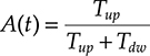
(8.33)
The ratio between the up time and the total operation time of the system can also be interpreted as the probability of founding the system working looking at it in a random instant. This is another possible definition of the availability of a system.
Besides the instantaneous availability, depending generally from time due to the fact that old systems tend to go out of work more frequently than new systems, the average availability is widely used, which is the average probability that in a fixed a time interval the system works in an instant of this time interval.
Mathematically it can be written as

(8.34)
where the total observation time has been identified with Δt, the up time is written as Δt− Tdw, which is the difference between the total observation time and the downtime and the function Tdw(τ) is a function defined only in the observation interval and equal to one when the system is out of work and to zero when it is correctly working.
Equation 8.34 can be read as the normalized average up time divided by the observation time, which is also the average probability to find the system working, observing it in a random instant during the observation time.
In the analysis of failures affecting systems that does not deteriorate sensibly with time, it is often assumed that the system working stabilizes up to a steady state in which the system characteristics does not depends on time. In this case, that reflects sufficiently well what happens in communication systems, a steady-state availability is defined as
![]()
(8.35)
In order to compare different survivability methods we will evaluate the corresponding value of the average steady state availability of the routed GLSPs using a simulation program. In order to evaluate the average GLSP availability, let us number the GLSPs (optical or MPLS depending on the case) that are routed through the network in an arbitrary order. Let us imagine that the simulation simulates NF failure events by extracting the failure starting instants tj with j = 1 to NF.
The simulation, in correspondence of each failure event, evaluates the duration of the different phases of protection or restoration and recovery for each individual GLSP and for each individual failure event. Let us consider the k-th GLSP; in correspondence of the generic h-th simulated failure it can be in one of three states:
Not involved in the failure
Restored after the failure via the network survivability mechanism
Impossible to restore via the survivability mechanism, restored when the network return in the working state that is when the failure is fully repaired
Let us assume a multiple survivability mechanism: for example, shared protection at the optical layer and Type 1 restoration at the MPLS layer coordinated through a hold-off time so as to avoid interlayer problems.
Simulating N F failure scenarios, let us assume that N0,k simulated failure events do not involve the k-th GLSP, in N1,k events, corresponding to the initial instants th1, it is recovered in a time
Finally, in N3,k = NF − N0,k − N1,k − N2,k failure events, the k-th GLSP is not recovered so that it turns up again only when the failure is completely repaired after a time
Thus the steady-state availability of the k-th GLSP can be evaluated as

(8.36)
where TT is the total simulated time that is the time elapsing from the simulation MPLS layer n start t1 = 0 to the instant in which, after the last failure event, the network is again in the working state.
Considering the average availability with respect to the NP GLSPs that are routed at the considered layer through the network it is finally obtained:

(8.37)
In cases in which both the recovery time and the failure repair time do not depend on the particular GLSP under examination and on the specific nature of the failure (that is, do not depends on the instant thj), Equation 8.37 becomes very simple.
Let us assume that we are observing a so long time that, for example, N1,k can be approximated as N1,k = P1(F) NF , where the probability P1(F) is the probability that, assuming to have a failure event, the considered GLSP is involved in the failure and can restored by the first survivability mechanism and analogously N2,k = P2(F) NF and N3,k = [1 − P1(F) − P2(F)] NF.
With these definitions Equation 8.38 becomes
![]()
(8.38)
where
τF is the interarrival time of the failure events.
〈T〉 is the average unavailability time of the generic GLSP in correspondence to a failure.
Besides network availability, when complex survivability strategies are implemented so that multiple failure can be faced, the so-called resilience factor (RF) is useful to evaluate the effectiveness of a survivability strategy. Let us imagine that a specific survivability strategy is able to face all single link failures (property always true for effective strategies) and a subset of multiple failure events.
Calling Sk ≡ {s1, s2, …} the set of all possible
among the m cable ducts at layer 0, the kth order resilience factor is defined as [26]

(8.39)
where
lsp(sj) is the cardinality of the set of working GLSPs that are interrupted by the contemporary failure of all the links in the set Sj
lspr(sj) is cardinality of the subset of those GLSPs that are restored without causing service disruption by the network protection mechanism
The normalization factor is derived from the number of links m.
The resilience factor of kth order can be also interpreted, if the failure events have the same probability, as the probability that an GLSP is restored in the presence of a random kth order failure event, and complete protection against k contemporary failures imply RFK = 1.
Since a network that is able to face k contemporary failures is in general also capable to manage a lower number of failures, the overall resilience factor RF is sometimes defined as

(8.40)
where F is the maximum number of contemporary failures that can be partially recovered and for our assumptions R1 = 1.
From the earlier discussion, it results that a key point in evaluating the survivability of a network is the analysis of the time that various elements of the recovery process, either protocols of hardware mechanisms, take to do their work.
Thus a detailed analysis of the recovery process is needed. When a failure occurs the network goes into the recovery state. The network in this state performs a series of operations aimed to perform recovery of the lost connections and return of the network to the normal state after the failure has been repaired.
These phases can be described as follows:
Phase 1: Fault detection
Phase 2: Fault localization and isolation
Phase 3: Fault notification
Phase 4: Recovery (protection/restoration)
Phase 5: Reversion (normalization)
Fault detection, localization, and notification phases are often joined together and called fault management. Reversion, also known as normalization process, is the mechanism bringing back the network from the recovery state, where the failed connections are reestablished using spare capacity, to the normal state. This process can be performed only after the physical repair of the failure and, among other elements, comprise the switch back of the connections affected by the failure to a working path.
It is to note that not always the working path after reversion is the same of those before reversion: as a matter of fact some restoration mechanisms reroute the connections in the reversion phase without any knowledge of their route before the failure occurs.
In order to perform failure recovery, alternative backup paths are required. These backup paths can be either set-up prior the failure or a posteriori. Given such possibilities, a range of different subphases in an a priori or a posteriori manner exists within the recovery process. The subphases and the associated elapsed times are illustrated in Table 8.8.
Table 8.8 Definition of the Failure Management Phases and the Corresponding Times

The restoration recovery time TRR depends on the type of restoration is used (compare Section 8.4.2.2). In particular we have

(8.41)
On the contrary, the protection recovery time TPR does not include the backup routing and backup signaling since the backup path was preestablished:
![]()
(8.42)
When a failure occurs, connections are lost until the traffic is switched over to the backup path. The amount of lost information due to a connection loss is a function of TPR or TRR and the number of LSRs directly corrupted by the failure. Generally, losses cannot be totally avoided by most of the protection mechanisms exceptions being 1 + 1 protection.
In the case of protection techniques, the time required to start the switchover is expressed as:
![]()
(8.43)
In case of restoration the switchover can be avoided: after restoration the new routes becomes working routes and when the failed capacity is restored it is included among the back-up resources.
8.5.2 Protection versus Restoration
In this section, we will consider the case of a single layer (the optical layer). One survivability mechanism is implemented in the network, either a type of protection or a type of restoration. Since link-dedicated protection is quite trivial within a GMPLS context, we will consider the following forms of optical path protection:
End-to-end 1 + 1 Dedicated Protection
End-to-end 1 + 1 Shared Protection
End-to-end 1:1 Shared Protection
As far as restoration is concerned, as we have already anticipated in the previous section, three methods of restoration are considered:
End-to-end GLSP restoration with complete re-provisioning (type 1 restoration):
A recovery path is not established before a failure. After the fault notification, the ingress layer 2 node starts the procedure to establish the whole failed GLSP to the egress node once again. This is a working involving both layer 2 and layer 1. However, it is not guaranteed that the process will succeed because the bandwidth is not prereserved and could be unavailable (it will not be possible to establish a recovery path). Two resource reuse procedures are associated to this kind of restoration technique: stub reuse and stub release. The stub reuse procedure consists in the fact that the recovery path may use parts of the working path not affected by the failure. The stub release procedure consists in the possibility that resources related to faulty connections are freed to be used by different connections for their recovery.
End-to-end GLSP restoration with presignaled recovery bandwidth reservation and no label preselection (type 2 restoration):
The bandwidth on the links that will constitute the recovery path is reserved by using signaling protocols, although the recovery path is not established. After a failure, the labels are chosen and the path is established by using a signaling protocol and, if necessary, the OXCs are rearranged. Even new routing through layer 2 topology could happen to exploit LSR grooming capability. The reserved resources may be shared among different recovery paths, but only when they are not affected by the same failures.
End-to-end GLSP restoration with presignaled recovery bandwidth reservation and label preselection (type 3 restoration):
Analogous to the method described earlier only faster, since the labels are assigned before the failure. Therefore, the necessity of OXC switching is signaled immediately after the fault notification.
These restoration methods can be applied at each layer of the network (but at layer 0 naturally), in this section we will consider them applied at layer 1 and we will compare their performances with those of the different protection mechanisms first under a qualitative point of view and then with a quantitative comparison.
8.5.2.1 Bandwidth Usage
Dedicated protection uses exactly the same bandwidth for protection that for working GLSPs. Shared protection is a bit more efficient. In 1:1 protection, the spare bandwidth is used for low-priority traffic, generally best effort services. In this way also the protection bandwidth is used during the normal network working.
Restoration with presignaled GLSPs and reserved bandwidth is generally slight better than shared protection. On the contrary, restoration with complete reprovisioning exploits the bandwidth at best.
8.5.2.2 Recovery Time
All protection mechanisms, due to the preprovision of the protection path, are very fast. The SDH/SONET standard of 50 ms between the failure and the complete service resto-ration is the reference for these methods. Restoration with presignaling and bandwidth reservation has a speed similar to protection, while the other two forms of restoration in general are quite slow.
8.5.2.3 Specific Protocols
Optical path 1 + 1 protection requires no real-time protocol, even if obviously the protection setup has to be advertised at the network elements and at the network manager. However, these communications does not condition the speed of the protection mecha-nism that is completely hardware.
In case of shared protection, a dedicated specific protocol has to be realized in order to manage the protection resources sharing and coordinate the protection switch on and switch off. The SDH/SONET automatic protection switching protocol (APS) is an example of such a protection dedicated protocol. Restoration processes are completely managed by the control plane and uses control plane standard protocols.
8.5.2.4 QoS Issues
In the cases of shared protection and, mainly, of restoration with complete reprovisioning of the path, it is difficult to guarantee some elements of the QoS, i.e., the network traversing time. If services with a high-level QoS are concerned, other survivability methods should be used.
8.5.2.5 Quantitative Comparison
To perform a quantitative comparison, for each survivability strategy we will consider three merit parameters. First is the survivability cost efficiency CE, which is the percentage of the overall cost expended for working equipment.
In other words,

(8.44)
This parameter represents somehow the results of the design. Besides CE we will consider. the average GLSP availability, or better the so-called unavailability (U = 1 − A), and finally the parameter RF2 to characterize the behavior in front of double failure events.
The simulation was carried out using the parameters summarized in Tables 8.7 and 8.9 and the main results, which are weakly dependent on traffic as far as the network is correctly dimensioned, are summarized in Table 8.10.
The first thing to be noticed is that dedicated protection absorbs about 64% of the network cost to deploy protection resources. This is due to the fact that the network connectivity is quite low so that protection paths are quite longer with respect to working paths. This causes DWDM systems used for protection to be much more costly than those used for working traffic. Moreover the protection routes also have an higher number of hops, forcing the nodes to devote a large amount of resources to process transit protection paths.
The situation is only a bit better for shared protection. Again, the poor network connec-tivity, which is frequently a characteristic of real geographical networks, forces protection paths to be frequently quite longer with respect of working path and sharing the protection capacity helps only partially. The result is that even when using shared protection a bit more that 50% of the network CAPEX is used to set up protection capacity.
Table 8.9 Design Parameters for the Design for Survivability of the North American Network

Table 8.10 Main Results of the Performance Evaluation of Different Survivability Strategies
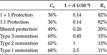
The situation is completely different considering restoration at the MPLS layer. As a matter of fact, while optical channel protection is constrained to maintain the optical channel in its wholeness protecting it as a single entity, MPLS restoration does not have this constraint.
What happens is that when restoration is in place and a link fails, layers 1 and 2 communicate through the common control plane and the GLSPs are individually restored not only by opening other optical paths exploiting free resources in layer 1, but also filling free spaces in already created optical paths and exploiting grooming to better distribute the traffic to be restored.
This causes a negligible increase of the cost of layer 2 (less than 2%) but the effect is strong and the final efficiency of restoration is near 70% if only the optical layer is considered or about 65% if all the network is taken into account.
The first type of restoration, without any preassignment of resources is slightly better due to the stub reuse and stub release procedures, while in the case of the other two restoration techniques, under the point of view of efficiency they have the same performances.
The value of the asymptotic availability, which we will use as a parameter, depends not only on the protection or restoration scheme, but also on the characteristics of the link failure process, on the repair time and on average time passing from the failure discovery to a complete traffic restoration.
In case of protection the time needed to restore a connection is assumed deterministic, while in case of restoration the recovery time is assumed a Gaussian random variable due to the need of running signaling protocols for the last two models of restoration and both routing and signaling for the first case. The time this protocol takes to provision and reserve restoration resources depends on the number of nodes to be traversed by the restored path and on the number of GLSPs to be restored. As a matter of fact, in our model, restoration manages each GLSP as an independent connection to be routed using available layer 1 capacity. As expected, the best availability is reached using dedicated protection, networks using bare rerouting restoration have the lower availability. Last, but not least, Table 8.10 shows the value of the reliability coefficient related to double failures.
The only scheme that has a reasonable probability to survive to a double failure is the dedicated optical channel protection. As a matter of fact, if two links will fail within a link repair time so that a double failure situation occurs, the only case in which traffic is lost is the case in which one failure affects a working path and the other the corresponding protection.
The values of RF2 are much smaller in the case of shared protection, due to the fact that in this case the traffic is lost either if both working and protection path fails and if two working paths sharing the same protection resources fails. In the considered case, the sharing degree (number of protection links shared by at least two working paths normalized to the number of protection links) is quite high.
A similar comment can be done regards restoration types 2 and 3, since in these cases restoration resources are reserved for restoration, even if not coupled with a particular working path. In this case the sharing is high so that RF2 is small.
8.5.3 Multilayer Survivability Strategies
The step beyond the use of a single survivability strategy is to use more than one contemporary method, in case at different layers. In the last section, the restoration was effectively based on cooperation between layers 1 and 2, due to the fact that all the MPLS LSPs hit by a failure were rerouted starting from their MPLS origin in layer 2. However, much better can be done if a coordinated multilayer strategy is adopted to manage a recovery mechanism at each layer.
8.5.3.1 Multilayer Survivability
Let us image that shared protection is adopted at Layer 1 with a network design suitable to face all single link failures. In case a multiple failure occurs and some GLSPs cannot be restored by layer 1 protection, layer 2 LSRs manage a restoration process to exploit free transport resources to reroute the affected LSPs.
Naturally the two processes have to be coordinated in order to avoid those problems that can occur in a bad designed multilayer restore mechanism. The most important phenomenon to be avoided is protection instability: if a path is protected at layer 1 and then also restored at layer 2, restoration can cause switching off optical power on the layer 1 protec-tion path. Layer 1 protection mechanism could interpret the fact as a new failure and try to protect the considered and other paths against it, with service disruption and the possibility to start an oscillatory phenomenon between the two layers.
The simpler way to coordinate two reliability mechanism located at different layers is to introduce a sufficiently long hold-off time at the upper layer so to give to the lower layer sufficient time to stabilize. More sophisticated methods however exists to avoid the increment of recovery time due to the fact that the hold-off time is the same for any failure event. These methods are based on the use of signaling protocols to advertise all the rel-evant network entities of the started protection switch.
It is also interesting to compare, at last in a qualitative way, multilayer reliability with a multistrategy single layer reliability, where, for example, both dedicated protection and wavelength level restoration are carried out by OXCs directly at the optical layer.
The basic multilayer approach advantage is that, in case the optical reliability mecha-nism does not work or is compromised by a multiple failure, the successive step is to route MPLS LSPs individually, exploiting the small granularity to perform more efficient restoration.
This is a principle similar to that of grooming, where complexity at layer 2 is traded with more effective exploitation of transmission capacity at layer 1. We will analyze multilayer survivability with the same method used in the previous section: we will design first the network for the required traffic, so deriving information on the network cost.
Table 8.11 Efficiency and Availability of Different Multilayer Survivability Strategies
Only Optical Layer Resources |
CE |
1 − A (×10−6) |
1 + 1 protection |
36% |
1.4 |
SP-R multilayer survivability |
25% |
0.8 |
R-R multilayer survivability |
45% |
1.3 |
Restoration type 2 |
65% |
10 |
We will use a three stage optimization, first optimizing the network for working traffic, then dimensioning the bottom layer survivability and at the end the upper layer survivability. The average availability is evaluated by simulation as in previous section. Two multilayer methods will be considered, assuming simple coordination through an hold-off time. The first method, which for simplicity we will call SP-R, is based on 1 + 1 optical GLSP at layer 1 and type 1 restoration at layer 2. This means that after a failure event, the MPLS LSR at layer 2 wait a certain time to let the optical layer to end its recovery attempt. After this time, all the LSR that has not been recovered by the optical layer has to be restored using already the available network resources to route them.
The second method, which briefly we will call R-R, comprises wavelength level type 3 restoration at layer 1 and LSR type 3 restoration at level 2. The survivability method efficiency and the average GLSP availability are reported in Table 8.11 in the conditions detailed in the previous section.
The two multilayer methods are both better with respect to single-layer methods, even if under different points of view. The R-R method attains almost the same availability of 1 + 1 optical protection, but at a much lower cost in terms of redundant equipment in the network. The SP-R method is quite expensive, but has the highest availability among the methods analyzed up to now.
Not only double failures can be efficiently faced, but also a few of triple and quadruple fail-ure events are recovered and a good recovery capability also exists in front of node failures. This property is shown in Table 8.12, where resilience factors of different degree are evaluated.
Besides the factor relative to multiple link failures, the resilience factor RFn relative to node failure is also reported. This new factor is defined in line with the definition of RFk as

(8.45)
Table 8.12 Resilience Degrees of Various Order for Two Multilayer Survivability Strategies
RF |
SP-R |
R-R |
RF2 |
1 |
1 |
RF3 |
0.85 |
0.82 |
RF4 |
0.77 |
0.71 |
RFn |
0.9 |
0.88 |
Rfn indicates the factor relative to full node failure.
where
N is the node number
lspn(j) is the total number of GLSPs processed in the absence of any failure by node j
The term lsp n0 (j) is added to the numerator of Equation 8.45 so to obtain a definition that gives one in case of full recovery, since local GLSPs cannot be recovered with any mean if the node fails.
8.5.3.2 QoS-Driven Multilayer Survivability
From a survivability point of view, multilayer restoration R-R and multilayer protectionrestoration SP-R are completely satisfactory, assuring excellent resilience against a large number of failure events and a very high GLSP survivability. Against this good perfor-mance, the cost to pay in terms of additional equipment to be deployed to provide the required spare capacity is very high. The cost of the network equipment is almost multiplied by two in the case of R-R and by more than two in the case of SP-R.
Sometimes it could be the right choice, due to the fact that the customer is willing to pay a high price to have a nine “9” survivability, it is the case of banks, other business customers like insurance, companies providing network based back-up of strategic data and so on.
In other cases however, this is clearly an excessive target bringing an excessive cost. This consideration, besides the very flexible structure of GMPLS, allowing to characterize GLSPs with a certain number of different tags, suggest that it should be the customer requirements, summarized in the service level agreement to drive the type of survivability to implement and consequently the service availability and cost.
In our model for QoS-driven multilayer survivability we will start mainly from Ref. [27], where a similar model was introduced and detailed. The main differences are that we will exploit multilayer structure of the network to benefit, when needed, to the possibility of layer 2 to manage reduced granularity LSPs with respect to the high capacity optical GLSPs and that we will assume that the network is designed and optimized for the specific level of traffic.
Even if in real networks, every LSPs has a specific bandwidth request, so that different classes of LSPs exist with respect to the capacity, we will continue to model the network as having a single type of LSP having fixed capacity. This assumption simplifies greatly the model and does not impact essentially results on survivability.
We will imagine, on the contrary, that when the layer 3 makes the request of a new LSP to layer 2 through the UNI interface, this request is characterized not only by the indication of the two end nodes, but also by the request of a certain QoS that, for what is our interest in this section, consists in the request of one of the available survivability classes.
In order to maintain a better control on the use of network resources, the network manager is imagined to force a constraint on the control plane, forcing not to allow the traffic allocated into a certain service class to go over a fixed percentage of the maximum traffic that the network can accept. Only the class one traffic, which does not require spare capacity, is allowed to grow as much as possible.
We will image that the network will offer to the client layer five possible classes of survivability, whose description is given in the following.
Service Class 0: Low Priority Traffic
This is constituted by unprotected LSPs that are routed using exclusively spare capacity that is planned to be used for shared protection or for restoration. When a failure occurs, the low-priority traffic that is routed onto the spare capacity, which has to be exploited for recovery is blocked, and the connection is lost.
This is the lower service class in terms of availability.
Service Class 1: Best Effort Traffic. This service class collects all the services, like web browsing and many other consumer services, that run onto a specifically provisioned capacity, but are not protected. If a failure occurs, on a working link where a best effort LSP is routed, it is lost up to the repair of the link.
Service Class 2: Standard Traffic. This is a class composed by LSPs that are protected via a type 1 restoration at the MPLS layer. It is important to notice that services of the classes 1 and 2 can run on the same physical fiber and even in the same optical GLSP. As a matter of fact, class 2 traffic restoration is managed by MPLS on layer 2. Thus if a fiber containing both class 1 and class 2 services is cut, the LSR that are at the ends of the involved GLSPs will start the rerouting of the failed class 2 LSPs, while will start signaling over the GMPLS network and through the UNI interface toward layer 3 to advertise that the involved best effort LSPs have been lost. In this case RF1 is very near to one, but not exactly equal.
Service Class 3: High Availability Traffic. This traffic is protected via a multilayer protection with the R-R method. This class of LSPs has a very high resilience toward many type of failure events, as we have evidenced in the last section, besides a complete recovery ability toward single and double link cut. Class 3 services cannot run on the same fibers where classes 1 and 2 services run, since they are protected also at the optical layer by a restoration mechanism. We will see that they can run in the same fibers of class 4 services, but not in the same wavelength.
Service Class 4: Mission Critical Traffic. This is the traffic that cannot be lost, but in cases of cataclysmic disasters like extended earthquakes or strategic nuclear attacks. The protection of these LSRs is with the SP-R method but with type 2 instead that type 1 restoration at MPLS layer. Moreover the SLA relative to this traffic type foresees a repair time of only 4 days against any type of link failure. It is to be noticed that LSPs belonging to class 4 can run on the same fibers where class 3 services run, but not on the same wavelengths. As a matter of fact, wavelengths accommodating class 4 services have to be protected at the optical layer as a whole, but this is not true for wavelength containing LSPs of class 3.
From the earlier discussion, it results that, as a consequence of the differentiation of the classes of service of the GLSPs, the wavelengths are also differentiated.
In particular, there are the following types of wavelengths:
Type 1 wavelengths: Containing working LSPs of classes 1 and 2 and spare capacity to be used by Layer 2 restoration processes. This last capacity can be occupied by low-priority traffic (service level 0).
Type 2 wavelengths containing service level 3 LSPs and spare capacity to be used by Layer 2 restoration processes. This last capacity can be occupied by low-priority traffic (service level 0).
Type 3 wavelengths containing service level 4 LSPs. Both protection and working paths are considered type 3 wavelengths, since they have no difference under a traffic load point of view but for the fact that at the receiver the working path is selected whenever possible.
Type 4 wavelengths that convey spare capacity to be used by restoration at layer 1 and can support low-priority traffic.
To dimension a network with a so complex traffic demand and survivability technique with IPL optimization in only two steps, one for capacity managing working traffic the other for capacity for use as a back-up is naturally possible under a theoretical point of view, but difficult to do with a realistic computation machine. It is to be noted however that the introduction of different classes of wavelength, practically segments the optical layer in different optical plans that have OXCs in common.
Thus it can be devised an algorithm based on the following steps:
Step 1: The first virtual network is dimensioned starting from the given layer 0 topology and assuming as traffic-only mission critical traffic. The fibers that will be equipped in this network will all be Type 3 fibers, all devoted to carry either working or protection Service Class 4 LSPs.
Step 2: A second virtual network is dimensioned starting from the same layer 0 topology and assuming as traffic only high-availability LSPs. The fibers that will be equipped in this network will all be Type 2 and Type 4 fibers and are tagged so to be possible to recognize their nature.
Step 3: A third virtual network is dimensioned starting from the same layer 0 topology and assuming as traffic only standard traffic and best effort GLSPs. The fibers that will be equipped in this network will all be Type 1 and Type 2 fibers and are tagged so to be possible to recognize their nature. This is the only step mixing two types of traffic, but it is managed easily due to the fact that best-effort traffic does not require back-up capacity.
In particular, the substeps are organized as follows:
A whole traffic matrix for the working traffic is created by merging standard and best-effort LSPs.
The overall traffic matrix is used to dimension the virtual network for the working part.
The traffic matrix relative to standard traffic only is retrieved and used to deploy protection capacity.
Step 4: OXC synthesis. The OXC occupying the same topological position in each virtual network are analyzed by merging them so to minimize their cost. The only exception is the OXC managing mission critical traffic that is not merged with other. The cost of these OXCs is on the other end recalculated doubling the cost of the interfaces to simulate 1 + 1 local interface protection. As far as the switch matrix is concerned, it is assumed to be doubled for protection in all the deployed OXCs and that this is already included in the cost of the OXC platform.
Table 8.13 Maximum Percentage of Traffic That Can Belong to a Specified QoS Class in the Example Discussed in This Section
Mission critical
5%
High reliability
20%
Standard
35%
Best effort
40%
Low priority (in addition to 100%)
30%
To show an example of OXC merging, let us image that in a certain node we have the following OXCs:
Virtual network 2: Number of out/in wavelength ports 22, platform 1
Virtual network 3: Number of out/in wavelength ports 12, platform 1
Final OXC design: Total number of ports 32, 1 platform (a second platform has to be eliminated)
Step 5: LSR synthesis. The LSR occupying the same topological position in each virtual network are analyzed by merging them so to minimize traffic. The operation is similar to that performed for OXC, but with no exceptions.
Step 6: Network synthesis. The fibers cannot be merged due to the limitations we have underlined previously, so this step only consists of putting all the network information into a single data base.
Step 7: Low-priority traffic is routed. It is to be noted that no further capacity is deployed and if the present back-up capacity is not sufficient to route a low priority traffic request, it is rejected by the network.
As in the other cases, after dimensioning a simulation is performed, where all the classes of service are present as foreseen by the network design. In the example whose results are reported in this section the mix of different LSR is reported in Table 8.13.
The result of the design and simulation is summarized in Figure 8.27 where the efficiency (indicating the CAPEX cost of the survivability) is related to the average availability of the selected types of LSR.

Figure 8.27 The efficiency (related to the CAPEX cost of the survivability) is related to the availability of the selected types of LSR for different types of Service Class (SC).
Looking at this figure a further efficiency reduction due to the OXC platform duplication is taken into account in the CE of the SP-R method.
8.6 Impact of ASON/GMPLS on Carriers OPEX
It is completely evident that the introduction of the ASON/GMPLS model is a sort of revolution in the way in which the carrier network is conceived and managed. The rationale of this revolution is in the great need of big carriers of reducing the OPEX related to the network so to prepare themselves to further network evolutions related to new services.
Intuition tells us that if all the network is managed through an automated and unique control plane, OPEX should decrease with respect to a situation in which the network layers are managed separately and in managing the transport layer several manual operations are needed.
However, we also know that intuition is not always reliable, thus carriers have carried out several studies to quantify the OPEX advantages related to the introduction of the new network paradigm. This quantification is also needed since this technology step implies the investment of relevant capital needed to buy new equipment or to update the deployed equipment so to be compatible with the new control plane. Besides equipment capitals, training of network personnel to the new procedures, change of carriers organization to reflect the new network structure are all costs that have to be paid to implement the new control plane.
A so big project cannot be executed without a detailed business plan pointing out costs and benefits and describing the impact of the project on the carrier business. Among the studies that has been done to try to determine the benefits of ASON/GMPLS we will follow the work presented in Refs. [28,29] both in the method and in the results.
In order to evaluate the OPEX expensed a model of the process implemented by the carrier to manage the network has to be done. This process is composed not only of technical activities, like network maintenance and technical personnel training to use and maintain new equipment, but also by sales and marketing activity to promote and sell new services, administration activity to control the company general working and other nontechnical processes that are fundamental for a good carrier working.
In order to model this complex set of activities, the model developed i [28,29] is based on an activity graph, which correlate various activities in terms of cause and effect. In particular, each activity is connected with other activities with oriented branches, tagged with a probability. This is the probability that if the carrier is carrying on the activity at the beginning of the branch, the activity at the end of the branch also will be needed.
A very simple example is given in Figure 8.28 where the graph relative to the process of repairing a failed card in an equipment is shown in detail. In Figure 8.29 a small part of the graph of Figure 8.28 is isolated to show how every element of the graph is tagged with a record containing the main element that are needed to evaluate the impact of the considered step on the cost of the overall activity represented by the graph.
The considered example regards a spot process of the reactive type: this means that the process happens at random instants as a reaction to a causing event, in this case the individuation of a failed card in an equipment. All spot events have a trigger; if the event is of the reaction type the trigger is an external event, if the event is a direct action (e.g., the planned substitution of a working but obsolete equipment) the trigger is the arrival of the time at which the action was planned.

Figure 8.28 Activity graph relative to the process of repairing a failed card in an equipment.

Figure 8.29 A small part of the graph of Figure 8.28 showing associated tags.
Besides spot processes, carriers implement a great number of recurring processes that periodically happen. In this case the graph does not have a trigger, but it is a closed loop containing a delay to regulate the periodicity of the event. A third type of processes are the continuous processes; these are the activities that never stop and constitute the base of the carrier work.
In particular circumstances a process can activate other processes starting their trigger. This causes a strong dependence of the operational processes one from the other. Some dependencies however can be neglected since they are so rare that do not impact the OPEX in a significant way.
The analysis proceeds by creating a complete description of the business activity of a big carrier via process diagrams and analyzing how the processes and the corresponding diagrams are changed by the introduction of ASON/GMPLS.
Thus operational models of the two carriers are defined before and after ASON/GMPLS. Since we tag every graph branch with a probability and every graph node with a double tag, we can calculate the cost and time needed to carry out the activity. For can every activity we can define an activity cost as the weighted average of the cost of every possible route through the activity graph connecting the activity start with the activity end. The weight of a route is naturally the overall probability that the route will take place.
Beside the activity cost, an average activity time is also evaluated, which is sometimes needed to take into account the fact that some activities cannot start again if they are still ongoing. Once the models are set up, we can evaluate the overall OPEX expenditure of the carrier. This is estimated by adding all the costs of parallel recurring or continuous activities.
As far as the spot activities are concerned, their costs are weighted with the probability of the trigger, so to take into account the fact that they are not continuous. Here we will not report the real activity graphs of the most complex activities, and much more details are reported in Refs. [28,29].
We will limit our self to list the main activities and the impact of the introduction of ASON/GMPLS on them. The main activities are all periodical or continuous, thus we will not repeat this every time.
Cost of failure free network operation: This is the base cost to take the network operational in a failure-free situation: it includes the cost of electrical power, building leasing for central offices, fiber leasing if it is the case, permissions for traversing private properties or to bring cables in private buildings, taxes on the ownership of the infrastructure and so on. This cost is heavily impacted by ASON/GMPLS due to the change of several equipments and to the substitution of preprovisioned protection with restoration in several areas of the network with a consequent reduction of the number of network equipments.
Routine operations: This is the cost related to all actions aimed to maintain the network in an efficient working status, maintaining the ability to face a possible failure. The main actions performed here aim at monitoring the network and its services. Therefore, the actions involved include the following:
Periodic verification of the equipment performances and services quality versus existing SLAs.
Management of the spare parts warehouses and activity to assure spare parts availability when a failure occurs.
Software management in terms of patches and new releases installation and bugs tracking.
Alarms management with all the activities aimed to failure identification, verification, and repair.
Network configuration management in terms of keeping track of changes in the network derived from failures or from equipment substitution due to preventive replacement of old or obsolete equipment.
Routine operations are influenced by ASON/GMPLS in two different ways. On one side, faster and more effective network reconfiguration allows the reduction of fail-ure-related service disruptions and consequently a more effective and less expensive process of intervention when a failure occurs.
On the other hand, software management will become more complex and expensive due to the introduction of a much more complex control plane.
Operational network planning: This is the set of actions that aim to maintain the network efficient and optimized. In a traditional transport network they are mainly manual operations carried out with the support of the TMN network manager and of off-line network optimization tools, often included into the TMN software. If ASON/GMPLS is used, these actions are mainly constituted by traffic engineering that, as we have seen in Section 8.3, are needed not to allow the network to slide very far from an optimized GLSPs routing. Since the ASON/GMPLS network is more complex, it is probable that this activity will be more expensive, even if it will be supported by more powerful tools.
Marketing: This is the traditional activity of customer base enlargement and customer maintenance through service promotions, new billing schemes introduc-tion and advertisement and so on. In correspondence with the introduction of ASON/GMPLS, it is reasonable to assume that new service bundles will be introduced so increasing the marketing expenses. On the other hand, even if this does not appear in our model, this will also bring new revenues.
Service management: These are all the activities related to offering, delivery, and managing end user services. Since this is a category quite important both for its absolute impact on carrier OPEX and for the impact of ASON/MPLS on it, it is worth doing a detailed analysis dividing this activity into subactivities.
Service offering: This is the process related to the preparation of the offering for the end customer in terms of service SLA and price. The sales department negotiates the terms and conditions of the offer with the customer, and does an inquiry as to whether the connection request can be handled by the standard mechanisms and infrastructure.
For nonstandard connection inquiries, a separate project is triggered. Then the offer is sent to the customer.
Service provisioning: This is the process related to the effective service setup after a contract has been subscribed with the end customer. After contract registration, a service provisioning project starts involving various parts of the carrier organization. At the end of the project, after a final test of the service by the carrier test department, the final customer is enabled to use the new service. A detailed action graph for service delivery is reported in Ref. [29].
Service cease: This is the process related to the discontinuation of a service after the end of the contract with the end customer.
Service move or change: Often moving or changing a connection is one of the most complex operations. It involves all three previous processes: contract update, new connection setup, and release of the previous connection. The customer’s request for change is handled by the sales department as a service offer process, checking again for the availability of resources. The sales department then generates orders for the service provisioning and cease process that are implemented through coordination from the Project Management department. At the same time, the client is receiving updates on the new installation.
Technologies automating some of the network operation allow the cost for service provisioning to be significantly reduced, because the signaling can be done via standardized interfaces (UNI and NNI), without requiring manual intervention. This means that the cost of setting up a new connection decreases greatly. In this case, the service offer and provisioning processes will change fundamen-tally. Since service delivery will now be automated and executed on the pure machine level, correct agreements and regulations must be negotiated by the sales department and implemented well before in the form of SLAs. The use of GMPLS technologies and the possibility to offer dynamic services are strongly interconnected issues.
The strongest impact of dynamic services is on the pricing and billing pro-cess. Fixed price services (e.g., leased lines) will definitely be cheaper in pricing and billing than dynamic services. For dynamic services, it is much more dif-ficult (and thus more expensive) to correctly assign costs to customer accounts. Calculating a new price for a new service is more expensive than just applying a traditional pricing scheme.
As a conclusion, provisioning of new services, especially when the setup of a new connection is needed, is quite cheaper both due to the easier process and to the absence of errors due to the elimination of manual operations. On the other hand, the process carried out by the sales department is more complicated and thus more expensive.
In analyzing the activity graphs and the related costs, it becomes evident that the greater OPEX cost element is the labor cost and it is also the most impacted by the transition to ASON/GMPLS.
Thus we will start our analysis from labor cost. This will be evaluated by detailing exactly the level of personnel that is needed and estimating the labor cost on the average over European nations and over United States. This average is done both using official statistics and doing a set of interviews with carriers to confirm them [29]. Naturally there is a difference between labor cost in Europe and in United States, but the percentage impact of ASON/GMPLS is not relevantly different [30,31].
It is natural to divide the carriers in two categories: incumbent carriers and competitive carriers. Incumbent carriers are characterized by a large, well-structured organization by a set of coded processes (probably relater to global quality certifications) and by the owner-ship of almost all the network they use to deliver services.
On the contrary, competitive carriers have a lighter organization and the general cost of a process is smaller both for the simpler organization and for the lighter structure. On the other hand, competitive carriers have higher costs in terms of consultancy services from the vendors since generally a set of activities that an incumbent operated through its own organizations are delegated to vendors by competitive carriers.
In Figure 8.30 the labor cost related to service management for a European incumbent carrier is shown considering a traditional network architecture and an architecture imple-menting ASON/GMPLS control plane.
The costs are divided into the processes we have considered in the previous analysis and the cost related to each process is further divided considering the carrier professional group carrying on the work. Costs are reported in normalized units.

Figure 8.30 Service management labor cost for an incumbent carrier considering a traditional network and an architecture implementing ASON/GMPLS control plane.
(After Pasqualini, S. et al., IEEE Commun. Mag., 6, 28, 2005.)
The first observation is that network automation reduces drastically the network man-agement costs needed in a traditional network, for example, to provision a new connection or to reroute a connection. These operations that require a relevant amount of manual work in a traditional network are completely automated via the control plane.
The counterpart is that the carrier front end, especially the sales group, has to face a more difficult work, absorbing more costs than in the traditional case. This is evident in Figure 8.31 where labor cost for service management processes is reported per professional group.

Figure 8.31 Service management labor cost for processes per professional group.
(After Pasqualini, S. et al., IEEE Commun. Mag., 6, 28, 2005.)

Figure 8.32 Global result for the overall OPEX of an incumbent carrier.
(After Pasqualini, S. et al., IEEE Commun. Mag., 6, 28, 2005.)
Taking into account all the changes, labor cost related to service management decreases about 52% with the introduction of ASON/GMPLS. A similar analysis can be carried out with North American costs deriving a reduction of the labor cost related to service management of about 42%. This is due to the fact that the difference between high-level and low-level employees in terms of compensation is much more evident in North America. The spared personnel in the network operation area is mainly con-stituted by technicians, warehouse workers, and similar professional figures that are located in the middle or lower part of the organization while the number of managers is less affected.
Thus the percentage OPEX spared is smaller. However, the result is in any case impressive, taking into account that we have considered the most critical part of the carrier OPEX.
The global result, obtained considering the overall OPEX of an European carrier, is shown in Figure 8.32. The overall sparing related to the introduction of ASON/MPLS is 24% (20% with U.S. numbers).
This is an important result if we consider that the annual OPEX of an average incum-bent carrier is around 70% of the overall carrier expenditure, a figure of the order of €3 billion for a medium European incumbent carrier. The results in the case of a competi-tive carrier are only slightly different due to the different weight of internal process structure.
We will give only, as an example, the result relative to the service management for a competitive European carrier. The plot, analogous to that of Figure 8.30, is reported in Figure 8.33. The percentage OPEX spare is of the same order of magnitude of that fore-casted for the incumbent, demonstrating that, if ASON/GMPLS will maintain its promises it is a good step in the right direction.

Figure 8.33 Global result for the overall OPEX of a competitive carrier.
(After Pasqualini, S. et al., IEEE Commun. Mag., 6, 28, 2005.)
REFERENCES
1.. ITU-T Recommendations regarding ASON standard architecture
G.8080/Y.1304: Architecture for the automatically switched optical network (ASON)
G.807/Y.1302: Requirements for automatic switched transport networks (ASTN) Call and Connection Management
G.7713/Y.1704: Distributed call and connection management (DCM) .
G.7713.1/Y.1704.1: DCM signalling mechanism using PNNI/Q.2931
G.7713.2/Y.1704.2: DCM signalling mechanism using GMPLS RSVP-TE
G.7713.3/Y.1704.3: DCM signalling mechanism using GMPLS CR-LDP Discovery and Link Management
G.7714/Y.1705: Generalized automatic discovery techniques
G.7715/Y.1706: Architecture and requirements of routing for automatic switched transport network
G.7716/Y.1707: Architecture and requirements of link resource management for automatically switched transport networks
G.7717/Y.1708: ASTN connection admission control. Other Related Recommendations .
G.872: Architecture of optical transport networks
G.709/Y.1331: Interface for the optical transport network (OTN) .
G.959.1: Optical transport network physical layer interfaces
G.874: Management aspects of the optical transport network element
G.874.1: Optical transport network (OTN) protocol-neutral management information model for the network element view
G.875: Optical transport network (OTN) management information model for the network element view
G.7041/Y.1303: Generic framing procedure (GFP)
G.7042/Y.1305: Link capacity adjustment scheme (LCAS) for virtual concatenated signals
G.65x: Series on optical fibre cables and test methods
G.693: Optical interfaces for intra-office systems
G.7710/Y.1701: Common equipment management function requirements
G.7712/Y.1703: Architecture and specification of data communication network
G.806: Characteristics of transport equipment. Description methodology and generic functionality
2.. OIF Implementation Agreements for ASON/GMPLS coordination
OIF-UNI-01.0: User Network Interface (UNI) 1.0 Signaling Specification (October 2001)
OIF-UNI-01.0-R2-Common: User Network Interface (UNI) 1.0 Signaling Specification, Release 2: Common Part
OIF-UNI-01.0-R2-RSVP: RSVP Extensions for User Network Interface (UNI) 1.0 Signaling, Release 2 (February 2004)
OIF-UNI-02.0-Common: User Network Interface (UNI) 2.0 Signaling Specification: Common Part .
OIF-UNI-02.0-RSVP: User Network Interface (UNI) 2.0 Signaling Specification: RSVP Extensions for User Network Interface (UNI) 2.0 (February 2008)
OIF-CDR-01.0: Call Detail Records for OIF UNI 1.0 Billing (April 2002) .
OIF-SEP-01.0: Security Extension for UNI and NNI (May 2003)
OIF-SEP-02.1: Addendum to the Security Extension for UNI and NNI (March 2006)
OIF-SLG-01.0: OIF Control Plane Logging and Auditing with Syslog (November 2007)
OIF-SMI-01.0: Security for Management Interfaces to Network Elements (September 2003)
OIF-SMI-02.1: Addendum to the Security for Management Interfaces to Network Elements (March 2006)
OIF-E-NNI-Sig-01.0: Intra-Carrier E-NNI Signaling Specification (February 2004)
OIF-E-NNI-Sig-02.0: E-NNI Signaling Specification (April 2009)
OIF-ENNI-OSPF-01.0: External Network-Network Interface (E-NNI) OSPF-based Routing -1.0 (Intra-Carrier) Implementation Agreement (January 2007)
OIF-G-Sig-IW-01.0: OIF Guideline Document: Signaling Protocol Interworking of ASON/GMPLS Network Domains (June 2008)
3. Iqbal, A. A., Mahmood, W., Ahmed, E., Samad, K., Evaluation of distributed control signaling protocols in GMPLS, Proceedings of the Fourth International Conference on Optical Internet (COIN05), Chongqing University of Posts and Telecommunications, Chongqing, China, May 29-June 2, 2005.
4.. Duarte, S., Martos, B., Brestavos, A., Almeida, V., Almeida, J., Traffic characteristics and com-munication patterns in blogosphere, Proceedings of the International Conference of Weblogs and Social Media, Boulder, CO, s.n., March 26–28, 2007.
5.. Sheluhin, O., Smolskiy, S., Osin, A., Self Similar Processes in Telecommunications, Wiley, Chichester, England, s.l., 2007. ISBN-13: 978-0470014868.
6.. Bigos, W., Cousin, B., Gosselin, S., Le Foll, M., Nakajima, H., Survivable MPLS over opti-cal transport networks: Cost and resource usage analysis, IEEE Journal on Selected Areas in Communications, 25(5), 949–961 (2007).
7. Nabil, N., Mouftah, H. T. Optimum planning of GMPLS transport networks. International Conference on Transparent Optical Networks - ICTON 2006, Nothingham, s.n., pp. 70–73, June 18–22, 2006.
8.. Sabella, R., Settembre, M., Oriolo, G., Razza, F., Ferlito, F., Conte, G., A multilayer solution for path provisioning in new-generation optical/MPLS networks, Journal of Lightwave Technology, 21(5), 1141–1155 (2003).
9.. Tornatore, M., Maier, G., Pattavina, A., WDM network optimization by ILP based on source formulation, Proceedings of IEEE INFOCOM, New York, USA, pp. 1813—1821, June 23–27, 2002.
10.. Proestaki, A., Sinclair, M. C., Design and dimensioning of dual-homing hierarchical multi-ring networks, IEE Proceedings on Communications, 147(2), 96–104 (2000).
Song, Y., Wool, A., Yener, B., Combinatorial design of multi-ring networks with combined routing and flow control, Computer Networks: The International Journal of Computer and Telecommunications Networking, 41(2), 247–267 (2003).
12.. Binetti, S., Bragheri, A., Iannone, E., Bentivoglio, F., Mesh and multi-ring optical networks for long-haul applications, IEEE Journal of Lightwave Technology, 18(12), 1677 (2000).
13.. Ash, G. R., Traffic Engineering and QoS Optimization of Integrated Voice & Data Networks, Morgan Kaufmann, San Francisco, CA, s.l., 2006. ISBN-13: 978-0123706256.
14.. Anjalia, T., Scoglio, C., A novel method for QoS provisioning with protection in GMPLS networks, Computer Communications, 29, 757–764 (2006).
15. Minoux, M., Networks synthesis and optimum network design problems: Models, solution methods and applications, Networks, 19(3), 313–360 (2006).
16.. Tornatore, M., Maier, G., Pattavina, A., WDM network design by ILP models based on flow aggregation, IEEE Transactions on Networking, 15(3), 709–720 (2007).
17. Scheffel, M., Kiese, M., Stidsen, T., A Clustering Approach for Scalable Network Design, Munich University of Technology, Munich, Germany, 2007. Deliverable of German Ministry of Education and Research Project ID 01BP551.
18.. Nguyen, H. N., Habibi, D., Phung, V. Q., Efficient optimization of network protection design with p-cycles, Journal of Photonic Network Communications, 19(1), 22–31 (2010).
19.. Lucentini, M., Spaccamela, A. M., Approximate solutions of an integer linear programming problem with resource variations, Lecture Notes in Control and Information Sciences, 18, 207–219 (1979).
20.. Schrijver, A., Theory of Linear and Integer Programming, Wiley, New York, 1998. ISBN-13: 978-0471982326.
21. Verbrugge, S., Colle, D., Pickavet, M., Demeester, P., Common planning practices for network dimensioning under traffic uncertainty, Design of Reliable Communication Networks (DRCN) 2003, Banff, Alberta, Canada, October 19–22, 2003.
22.. Sugiyama, R., Takeda, T., Oki, E., Shiomoto, K., Network design method based on adaptive selec-tion of facility-adding and path-routing policies under traffic growth, Global Telecommunications Conference, GLOBECOM 2008, New Orleans, LA, IEEE, s.l., USA, November 30–December 3, 2008.
23. Naas, N., Mouftah, H. T., Efficient heuristics for planning GMPLS transport networks, Canadian Conference on Electrical and Computer Engineering, CCECE 2007, Vancouver, British Columbia, Canada, s.n., April 22–26, 2007.
24.. Fukumoto, T., Komoda, N., Optimal paths design for a GMPLS network using the Lagrangian relaxation method, Symposium on Computational Intelligence in Scheduling, SCIS ‘07, Honolulu, HI, IEEE, 2007.
25. Lacković, M., Mikac, B., Analytical vs. simulation approach to availability calculation of cir-cuit switched optical transmission network, Proceedings of the 7th International Conference on Telecommunications, ConTEL 2003, Zagreb, Croatia, IEEE, s.l., Vol. 2, pp. 743–750, 2003.
26. Sone, Y., Nagatsu, N., Imajuku, W., Jinno, M., Takigawa, Y., Optical path restoration scheme escalation achieving enhanced operation and high survivability in multiple failure scenarios, Network Innovation Laboratories, Public Presentation, NTT, 2007.
27. Ricciato, F., Listanti, M., Salsano, S., An architecture for differentiated protection against single and double faults in GMPLS, Photonics Networks Communications, 8(1), 119–132 (2004).
28.. Kirstadter, A., Iselt, A., Winkler, C., Pasqualini, S., A quantitative study on the influence of ASON/GMPLS on OPEX, International Journal of Electronics and Communications, 60(1), 1–4 (2006).
29.. Pasqualini, S., Kirstädter, A., Iselt, A., Chahine, R., Verbrugge, S., Colle, D., Pickavet, M., Demeester, P., Influence of GMPLS on network providers’ operational expenditures: A quantitative study, IEEE Communications Magazine, 6, 28–34 (2005).
30.. USA Bureau of Labor, National Compensation Statistical data, 2010, Public Report, http://www.bls.gov/data/ (accessed: July 2, 2010).
Organization for Economic Cooperation and Development, Unit Labor Cost working paper including detailed zone aggregation methodology, 2010, Public Report, http://stats.oecd.org/mei/default.asp?lang=e&subject=19&country=OEU (accessed: July 2, 2010).
32.. IETF RFCs related to the MPLS Architecture
IETF-RFC2205: Braden, R. (Ed.), Resource Reservation Protocol (RSVP)—Version 1 Functional Specification, September 1997, http://www.ietf.org/rfc/rfc2205.txt
IETF-RFC2370: Coltun, R. The OSPF Opaque LSA Option, July 1998, http://www.ietf.org/rfc/rfc2370.txt
IETF-RFC2748: Durham, D. (Ed.), The COPS (Common Open Policy Service) Protocol, January 2000, http://www.ietf.org/rfc/rfc2748.txt
IETF-RFC2903: Laat de, C., Gross, G., Gommans, L., Vollbrecht, J., Spence, D., Generic AAA Architecture, Experimental, August 2000, http://www.ietf.org/rfc/rfc2903.txt
IETF-RFC2904: Vollbrecht, J., Calhoun, P., Farrell, S., Gommans, L., Gross, G., de Bruijn, B., de Laat, C., Holdrege, M., Spence, D., AAA Authorization Framework, August 2000, http://www.ietf.org/rfc/rfc2904.txt
IETF-RFC3630:Katz, K. (Ed.), Traffic Engineering (TE) Extensions to OSPF Version 2, September 2003, http://www.ietf.org/rfc/rfc3630.txt
IETF-RFC4203: Kompella, K. (Ed.), OSPF Extensions in Support of Generalized Multi-Protocol Label Switching, October 2005
IETF-RFC4204: Lang, J. (Ed.), Link Management Protocol (LMP), October 2005, http://www.ietf.org/rfc/rfc4204.txt
IETF-RFC4940: Kompella, K., Fenner, B., IANA Considerations for OSPF, July 2007
33.. Griffith, D., Rouil, R., Klink, S., Sriram, K., An analysis of path recovery schemes in GMPLS opti-cal networks with various levels of pre-provisioning [aut. libro]. In Z. Zhang, A. K. Somani (Eds.) Proceedings of SPIE Optical Networking and Communications, Orlando, USA, September 7–11, 2003.
34.. Resea, B., Multiple hierarchical protection schemes for differentiated services in GMPLS networks, Proceedings International Conference on Information Technology: Research and Education, ITRE 2003, Newark, NJ, USA, August 10–13, 2003.
35.. Aweya, J. IP router architectures: An overview. International Journal of Communication Systems. Whiley, 14(5), 447–475 (2001).
36. Lawton, G. Routing laces dramatic changes. Computer. IEEE, 42(9), 15-17 (2009).
37.. Csaszar, A., et al. Converging the evolution of router architectures and IP networks. Networks. IEEE, 21(4), 8–14 (2007).