
Chapter 7
History of Computers
Most people take computers for granted today without even noticing their impact on society. To gain a better understanding of our digital world, this chapter examines the history of computing: hardware, software, and users. This chapter begins with the earliest computing devices before moving into the development of the electronic, digital, programmable computer. Since the 1940s, computers fall into four “generations,” each of which is explored. The evolution of computer software provides three overlapping threads: changes in programming, changes to operating systems, changes to application software. The chapter also briefly considers how computer users have changed as the hardware and software have evolved.
The learning objectives of this chapter are to
- Compare computer hardware between the four computer generations.
- Describe the impact that integrated circuits and miniaturization have played on the evolution of computer hardware.
- Describe shifts in programming from low level languages to high level languages including concepts of structured programming and object-oriented programming.
- Explain how the role of the operating system arose and examine advances in software.
- Discuss the changes in society since the 1950s with respect to computer usage and computer users.
In all of human history, few inventions have had the impact on society that computers have had. Perhaps language itself, the ability to generate and use electricity, and the automobile have had similar impacts as computers. In the case of the automobile, the impact has been more significant in North America (particularly in the United States) than in other countries that rely on mass transit such as trains and subways. But without a doubt, the computer has had a tremendous impact on most of humanity, and the impact has occurred in a shorter time span than the other inventions because large-scale computer usage only dates back perhaps 25–30 years. In addition to the rapid impact that computers have had, it is certainly the case that no other human innovation has improved as dramatically as the computer. Consider the following simple comparisons of computers from the 1950s to their present-day counterparts:
- A computer of the 1950s cost hundreds of thousands of 1950s dollars, whereas computers today can be found as cheaply as $300 and a “typical” computer will cost no more than $1200.
- A computer of the 1950s could perform thousands of instructions per second, whereas today the number of instructions is around 1 billion (an increase of at least a million).
- A computer of the 1950s had little main memory, perhaps a few thousand bytes; today, main memory capacity is at least 4 GB (an increase of perhaps a million).
- A computer of the 1950s would take up substantial space, a full large room of a building, and weigh several tons; today, a computer can fit in your pocket (a smart phone) although a more powerful general-purpose computer can fit in a briefcase and will weigh no more than a few pounds.
- A computer of the 1950s would be used by no more than a few people (perhaps a dozen), and there were only a few hundred computers, so the total number of people who used computers was a few thousand; today, the number of users is in the billions.
If cars had progressed like computers, we would have cars that could accelerate from 0 to a million miles per hour in less than a second, they would get millions of miles to a gallon of gasoline, they would be small enough to pack up and take with you when you reached your destination, and rather than servicing your car you would just replace it with a new one.
In this chapter, we will examine how computers have changed and how those changes have impacted our society. We will look at four areas of change: computer hardware, computer software, computer users, and the overall changes in our society. There is a separate chapter that covers the history of operating systems. A brief history of the Internet is covered in the chapter on networks, although we will briefly consider here how the Internet has changed our society in this chapter.
Evolution of Computer Hardware
We reference the various types of evolution of computer hardware in terms of generations. The first generation occurred between approximately the mid 1940s and the late 1950s. The second generation took place from around 1959 until 1965. The third generation then lasted until the early 1970s. We have been in the fourth generation ever since. Before we look at these generations, let us briefly look at the history of computing before the computer.
Before the Generations
The earliest form of computing was no doubt people’s fingers and toes. We use decimal most likely because we have 10 fingers. To count, people might hold up some number of fingers. Of course, most people back in 2000 b.c. or even 1000 a.d. had little to count. Perhaps the ancient shepherds counted their sheep, and mothers counted their children. Very few had much property worth counting, and mathematics was very rudimentary. However, there were those who wanted to count beyond 10 or 20, so someone invented a counting device called the abacus (see Figure 7.1). Beads represent the number of items counted. In this case, the abacus uses base 5 (five beads to slide per column); however, with two beads at the top of the column, one can either count 0–4 or 5–9, so in fact, each column represents a power of 10. An abacus might have three separate regions to store different numbers, for instance: the first and third numbers can range from 0 to 9999, and the middle number can be from 0 to 99999. We are not sure who invented the abacus or how long ago it was invented, but it certainly has been around for thousands of years.
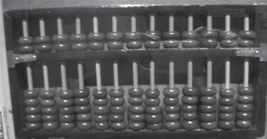
An abacus. (Courtesy of Jrpvaldi, http://commons.wikimedia.org/wiki/File:Science_museum_030.jpg .)
Mathematics itself was very challenging around the turn of the millennium between BC and AD because of the use of Roman numerals. Consider doing the following arithmetic problem: 42 + 18. In Roman numerals, it would be written as XLII + XVIII. Not a very easy problem to solve in this format because you cannot simply line up the numbers and add the digits in columns, as we are taught in grade school.
It was not until the Renaissance period in Europe that mathematics began to advance, and with it, a desire for automated computing. One advance that permitted the improvement in mathematics was the innovation of the Arabic numbering system (the use of digits 0–9) rather than Roman numerals. The Renaissance was also a period of educational improvement with the availability of places of learning (universities) and books. In the 1600s, mathematics saw such new concepts as algebra, decimal notation, trigonometry, geometry, and calculus.
In 1642, French mathematician Blaise Pascal invented the first calculator, a device called the Pascaline. The device operated in a similar manner as a clock. In a clock, a gear rotates, being moved by a pendulum. The gear connects to another gear of a different size. A full revolution of one gear causes the next gear to move one position. In this way, the first gear would control the “second hand” of the clock, the next gear would control the “minute hand” of the clock, and another gear would control the “hour hand” of the clock. See Figure 7.2, which demonstrates how different sized gears can connect together. For a mechanical calculator, Pascal made two changes. First, a gear would turn when the previous gear had rotated one full revolution, which would be 10 positions instead of 60 (for seconds or minutes). Second, gears would be moved by human hand rather than the swinging of a pendulum. Rotating gears in one direction would perform additions, and rotating gears in the opposite direction would perform subtractions. For instance, if a gear is already set at position 8, then rotating it 5 positions in a clockwise manner would cause it to end at position 3, but it will have passed 0 so that the next gear would shift one position (from 0 to 1), leaving the calculator with the values 1 and 3 (8 + 5 = 13). Subtraction could be performed by rotating in a counterclockwise manner.

In 1672, German mathematician and logician Gottfried Leibniz expanded the capability of the automated calculator to perform multiplication and division. Leibniz’s calculator, like Pascal’s, would use rotating gears to represent numbers whereby one gear rotating past 10 would cause the next gear to rotate. However, Leibniz added extra storage locations (gears) to represent how many additions or subtractions to perform. In this way, the same number could be added together multiple times to create a multiplication (e.g., 5 * 4 is just 5 added together 4 times). Figure 7.3 shows both Pascal’s (a) and Leibniz’s (b) calculators. Notice the hand crank in Leibniz’s version to simplify the amount of effort of the user, rather than turning individual gears, as with the Pascaline.
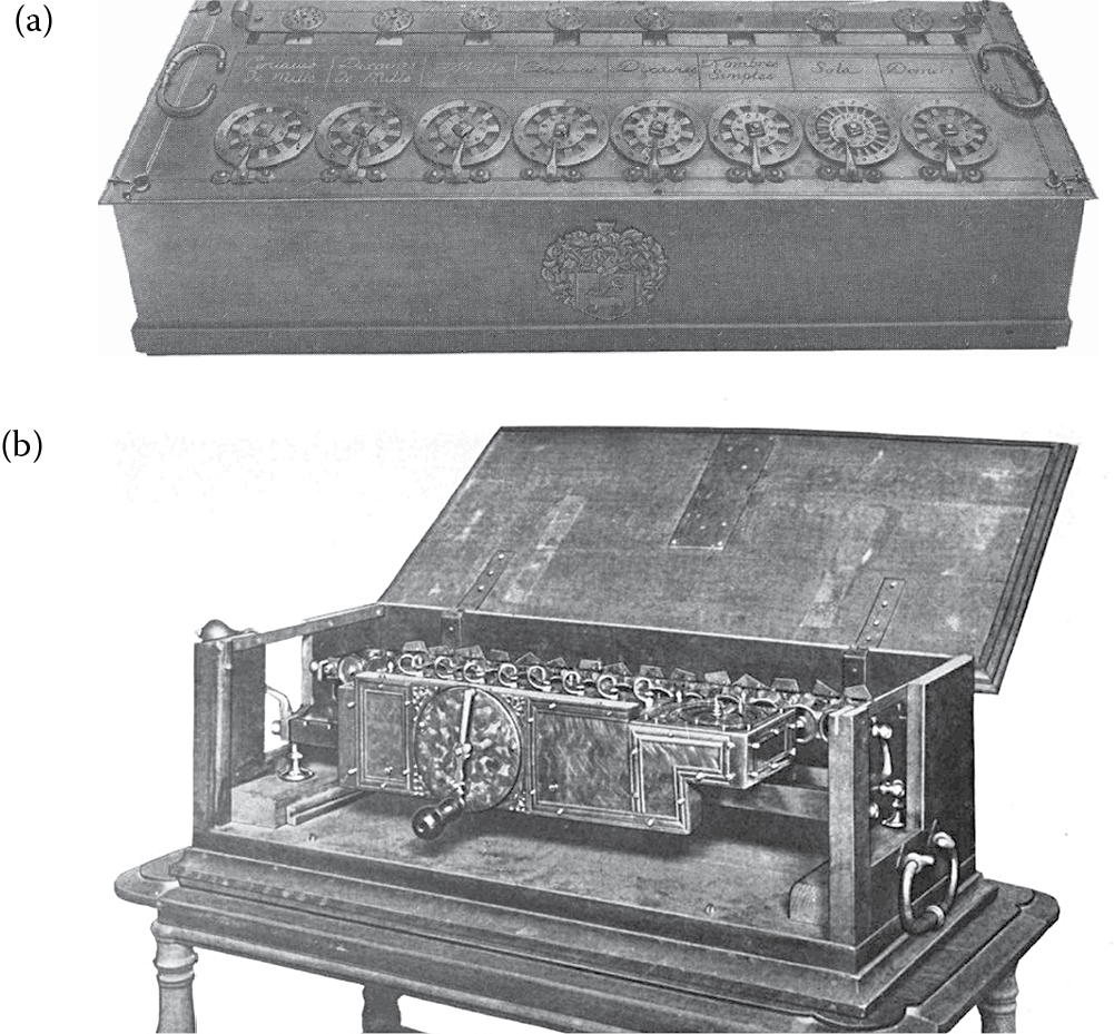
(a) Pascal’s calculator (Scan by Ezrdr taken from J.A.V. Turck, 1921, Origin of Modern Calculating Machines, Western Society of Engineers, p. 10. With permission.) and (b) Leibniz’s calculator. (Scan by Chetvorno, taken from J.A.V. Turck, 1921, Origin of Modern Calculating Machines, Western Society of Engineers, p. 133. With permission.)
In 1801, master weaver Joseph Marie Jacquard invented a programmable loom. The loom is a mechanical device that allows threads to be interwoven easily. Some of the threads are raised, and a cross-thread is passed under them (but above other threads). The raising of threads can be a time-consuming process. Hooks are used to raise some selection of threads. Jacquard automated the process of raising threads by punch cards. A punch card would denote which hooks are used by having holes punched into the cards. Therefore, a weaver could feed in a series of cards, one per pass of a thread across the length of the object being woven. The significance of this loom is that it was the first programmable device. The “program” being carried out is merely data that dictates which hooks are active, but the idea of automating the changes and using punch cards to carry the “program” instructions would lead to the development of more sophisticated programmable mechanical devices. Figure 7.4 illustrates a Jacquard loom circa end of the 1800s. Notice the collection of punch cards that make up the program, or the design pattern.
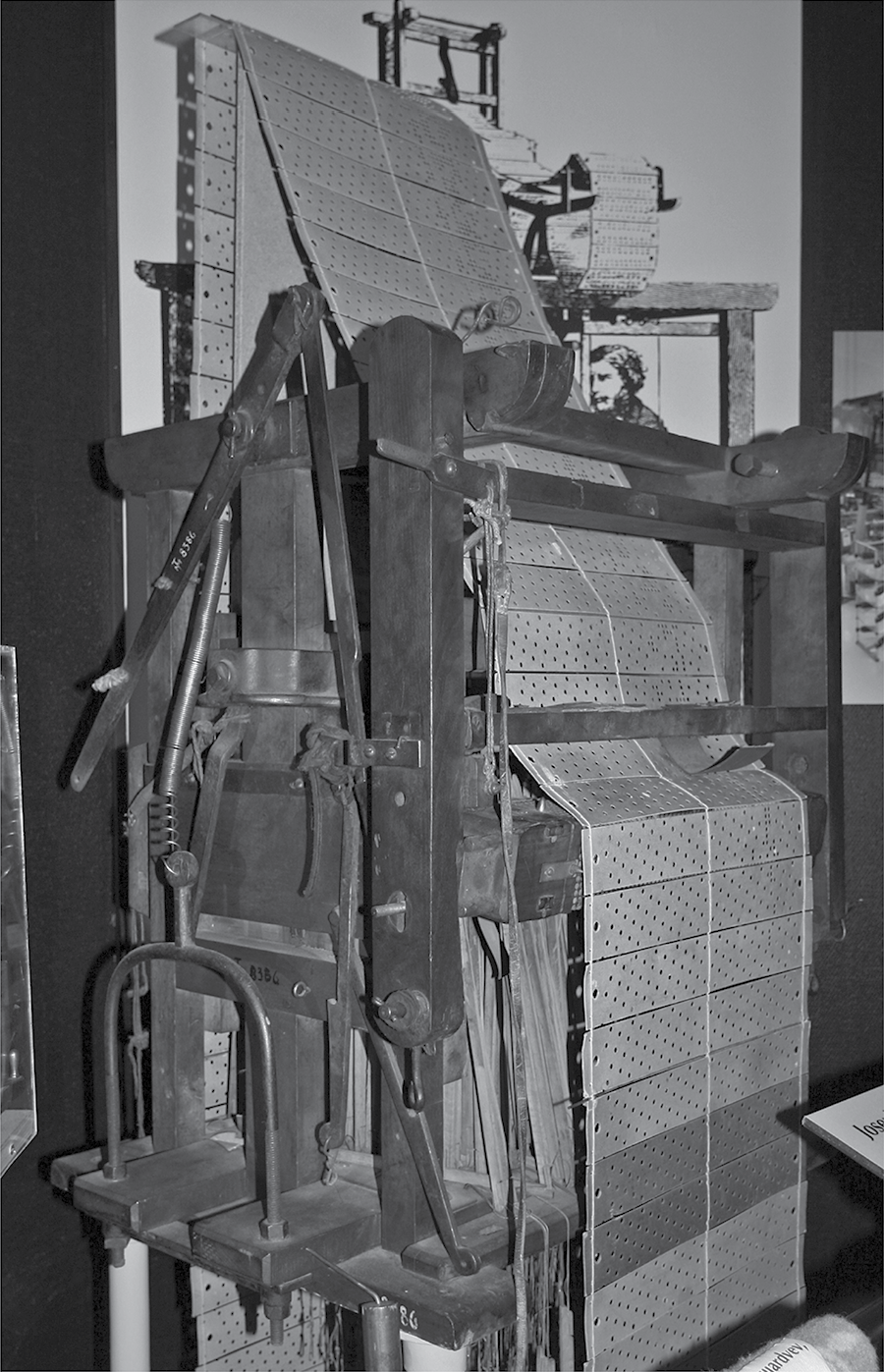
Jacquard’s programmable loom. (Mahlum, photograph from the Norwegian Technology Museum, Oslo, 2008, http://commons.wikimedia.org/wiki/File:Jacquard_loom.jpg .)
In addition to the new theories of mathematics and the innovative technology, the idea behind the binary numbering system and the binary operations was introduced in 1854 when mathematician George Boole invented two-valued logic, now known as Boolean logic.* Although this would not have a direct impact on mechanical-based computing, it would eventually have a large impact on computing.
In the early 1800s, mathematician Charles Babbage was examining a table of logarithms. Mathematical tables were hand-produced by groups of mathematicians. Babbage knew that this table would have errors because the logarithms were computed by hand through a tedious series of mathematical equations. These tables were being computed by a new idea, difference equations. Difference equations consist solely of additions and subtractions, but each computation could be very involved. Babbage hit on the idea that with automated calculators, one could perhaps program a calculator to perform the computations necessary and even print out the final table by using a printing press form of output. Thus, Babbage designed what he called the Difference Engine. It would, like any computer, perform input (to accept the data), processing (the difference equations), storage (the orientation of the various gears would represent numbers used in the computations), and output (the final set of gears would have digits on them that could be printed by adding ink). In 1822, he began developing the Difference Engine to compute polynomial functions. The machine would be steam powered. He received funding from the English government on the order of ₤17,000 over a 10-year period.
By the 1830s, Babbage scrapped his attempts at building the Difference Engine when he hit upon a superior idea, a general-purpose programmable device. Whereas the Difference Engine could be programmed to perform one type of computation, his new device would be applicable to a larger variety of mathematical problems. He named the new device the Analytical Engine. Like the Difference Engine, the Analytical Engine would use punch cards for input. The input would comprise both data and the program itself. The program would consist of not only mathematical equations, but branching operations so that the program’s performance would differ based on conditions. Thus, the new device could make decisions by performing looping (iteration) operations and selection statements. He asked a fellow mathematician, Lady Ada Lovelace, to write programs for the new device. Among her first was a program to compute a sequence of Bernoulli numbers. Lovelace finished her first program in 1842, and she is now considered to be the world’s first computer programmer. Sadly, Babbage never completed either engine having run out of money. However, both Difference Engines and Analytical Engines have been constructed since then using Babbage’s designs. In fact, in 1991, students in the UK constructed an Analytical Engine using components available in the 1830s. The cost was some $10 million. Figure 7.5 is a drawing of the Difference Engine on display at London’s Science Museum.
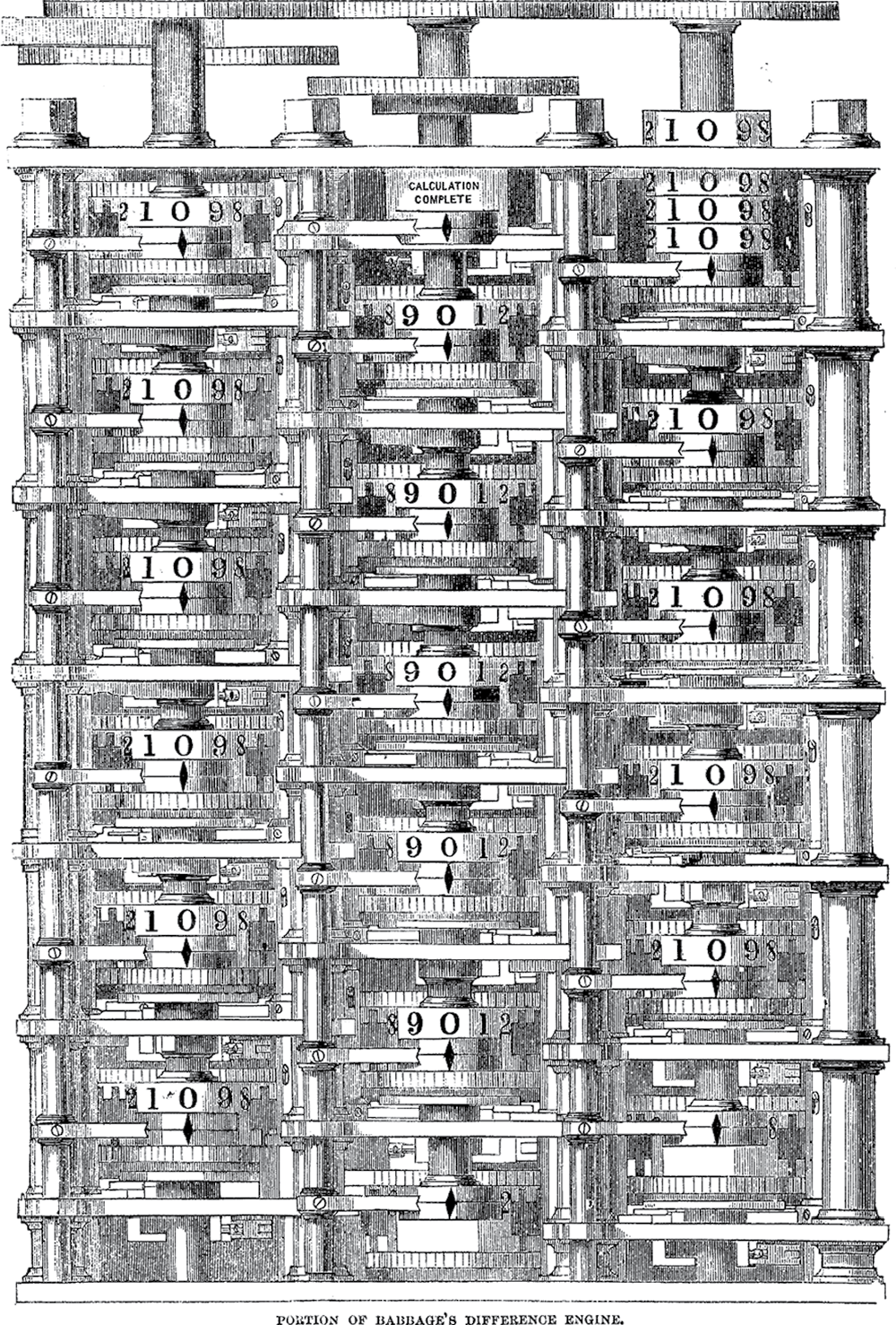
A difference engine. (From Harper’s New Monthly Magazine, 30, 175, p. 34. http://digital .library.cornell.edu/cgi/t/text/pageviewer-idx?c=harp;cc=harp;rgn=full%20text;idno=harp0030 - 1;didno=harp0030-1;view=image;seq=00044;node=harp0030-1%3A1. With permission.)
Babbage’s “computer” operated in decimal, much like the previous calculator devices and was mechanical in nature: physical moving components were used for computation. Gears rotated to perform additions and subtractions. By the late 1800s and into the 1900s, electricity replaced steam power to drive the rotation of the mechanical elements. Other mechanical elements and analog elements (including in one case, quantities of water) were used rather than bulky gears. But by the 1930s and 1940s, relay switches, which were used in the telephone network, were to replace the bulkier mechanical components. A drawing of a relay switch is shown in Figure 7.6. A typical relay switch is about 3 cm2 in size (less than an inch and a half). The relay switch could switch states more rapidly than a gear could rotate so that the performance of the computing device would improve as well. A relay switch would be in one of two positions and thus computers moved from decimal to binary, and were now referred to as digital computers.
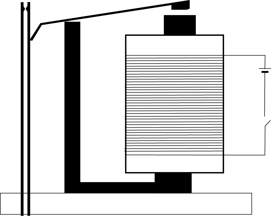
Electromagnetic relay switch. (Adapted from http://commons.wikimedia.org/wiki/File:Schema_rele2.PNG .)
First Generation
Most of the analog (decimal) and digital computers up until the mid 1940s were special-purpose machines—designed to perform only one type of computation (although they were programmable in that the specific computation could vary). These included devices to compute integral equations and differential equations (note that this is different from the previously mentioned difference equations).
By the time World War II started, there was a race to build better, faster, and more usable computers. These computers were needed to assist in computing rocket trajectories. An interesting historical note is that the first computers were not machines—they were women hired by the British government to perform rocket trajectory calculations by hand! Table 7.1 provides a description of some of the early machines from the early 1940s.
Early Computers
|
Name |
Year |
Nationality |
Comments |
|
Zuse Z3 |
1941 |
German |
Binary floating point, electromechanical, programmable |
|
Atanasoff-Berry |
1942 |
US |
Binary, electronic, nonprogrammable |
|
Colossus Mark 1 |
1944 |
UK |
Binary, electronic, programmable |
|
Harvard (Mark 1) |
1944 |
US |
Decimal, electromechanical, programmable |
|
Colossus Mark 2 |
1944 |
UK |
Binary, electronic, programmable |
|
Zuse Z4 |
1945 |
German |
Binary floating point, electromechanical, programmable |
The Allies also were hoping to build computers that could crack German codes. Although completed after World War II, the ENIAC (Electronic Numerical Integrator and Computer) was the first digital, general-purpose, programmable computer, and it ended all interest in analog computers. What distinguishes the ENIAC from the computers in Table 7.1 is that the ENIAC was general-purpose, whereas those in Table 7.1 were either special purpose (could only run programs of a certain type) or were not electronic but electromechanical. A general-purpose computer can conceivably execute any program that can be written for that computer.
Built by the University of Pennsylvania, the ENIAC was first made known to the public in February of 1946. The computer cost nearly $500,000 (of 1940s money) and consisted of 17,468 vacuum tubes, 7200 crystal diodes, 1500 relays, 70,000 resistors, 10,000 capacitors, and millions of hand-soldered joints. It weighed more than 30 tons and took up 1800 ft2. Data input was performed by punch cards, and programming was carried out by connecting together various electronic components through cables so that the output of one component would be used as the input to another component (Figure 7.7). Output was produced using an offline accounting machine. ENIAC’s storage was limited to about 200 digits. Interestingly, although the computer was a digital computer (which typically means a binary representation), the ENIAC performed decimal computations. Although the ENIAC underwent some upgrades in 1947, it was in continuous use from mid 1947 until October 1955. The ENIAC, with its use of vacuum tubes for storage, transistors, and other electronics for computation, was able to compute at the rate of 5000 operations per second. However, the reliance on vacuum tubes, and the difficulty in programming by connecting components together by cable, led to a very unreliable performance. In fact, the longest time the ENIAC went without a failure was approximately 116 hours.
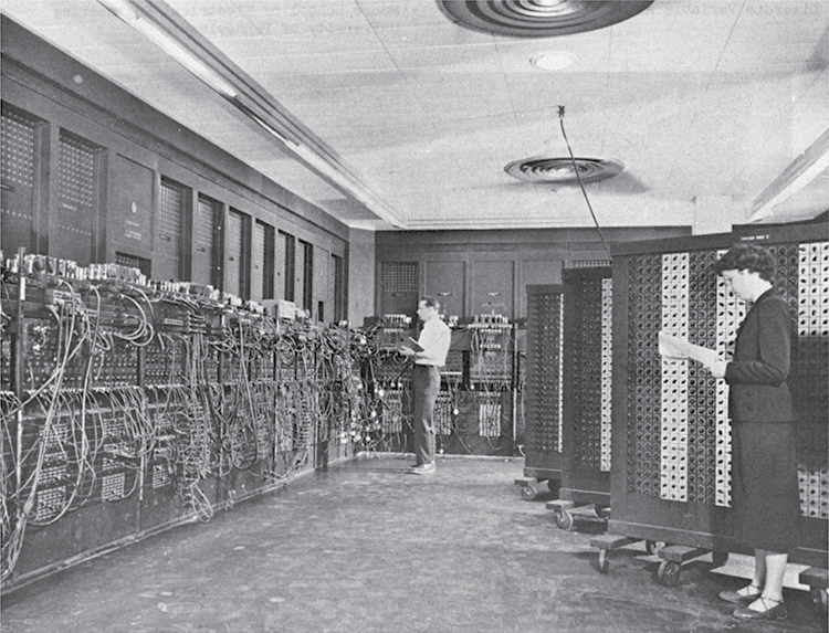
Programming the Electronic Numerical Integrator and Computer (ENIAC). (Courtesy of http://commons.wikimedia.org/wiki/File:Eniac.jpg , author unknown.)
The ENIAC, and other laboratory computers like it, constitute the first generation of computer hardware, all of which were one-of-a-kind machines. They are classified not only by the time period but also the reliance on vacuum tubes, relay switches, and the need to program in machine language. By the 1940s, transistors were being used in various electronic appliances. Around 1959, the first computers were developed that used transistor components rather than vacuum tubes. Transistors were favored over vacuum tubes for a number of reasons. They could be mass produced and therefore were far cheaper. Vacuum tubes gave off a good deal of heat and had a short shelf life of perhaps a few thousand hours, whereas transistors could last for up to 50 years. Transistors used less power and were far more robust.
Second and Third Generations
Around the same time, magnetic core memory was being introduced. Magnetic core memory consists of small iron rings of metal, placed in a wire-mesh framework. Each ring stores one bit by having magnetic current rotate in either clockwise or counterclockwise fashion.
It was these innovations that ushered in a new generation of computers, now referred to as the second generation. Figure 7.8 illustrates these two new technologies. Figure 7.8 provides a comparison between the vacuum tube and transistor (note the difference in size), and Figure 7.8 shows a collection of magnetic core memory. The collection of magnetic cores and wires constitute memory where each ring (at the intersection of a horizontal and a vertical wire) stores a single bit. The wires are used to specify which core is being accessed. Current flows along one set of wires so that the cores can retain their charges. The other set of wires is used to send new bits to select cores or to obtain the values from select cores.
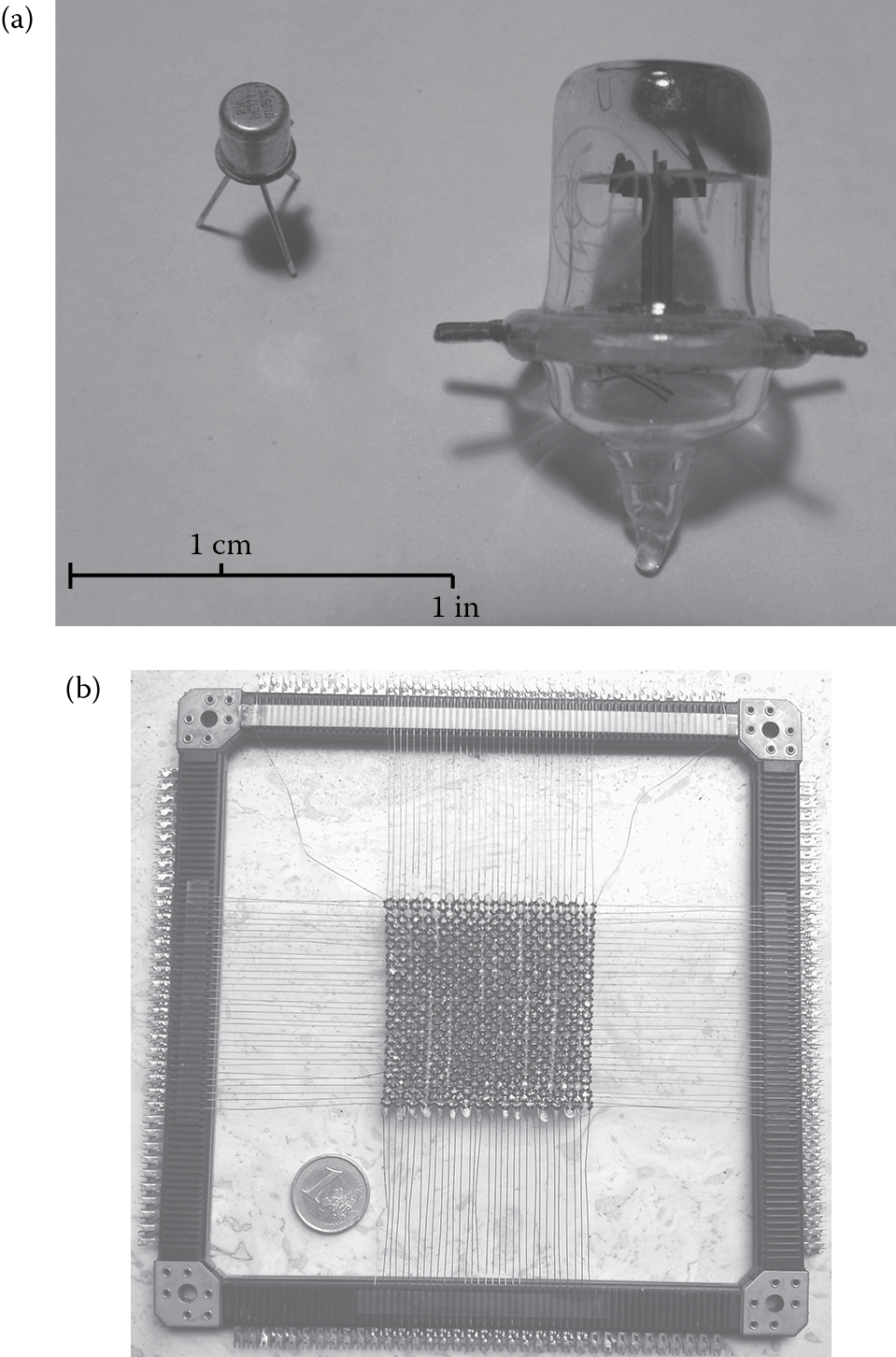
The vacuum tube and transistor (a) (Courtesy of Andrew Kevin Pullen, http://commons.wikimedia.org/wiki/File:955ACORN.jpg .) and magnetic core memory (b) (Courtesy of HandigeHarry, http://commons.wikimedia.org/wiki/File:Core_memory.JPG .)
The logic of the computer (controlling the fetch–execute cycle, and performing the arithmetic and logic operations) could be accomplished through collections of transistors. For instance, a NOT operation could be done with two transistors, an AND or OR operation with six transistors, and a 1-bit addition circuit with 28 transistors. Therefore, a few hundred transistors would be required to construct a simple processor.
By eliminating vacuum tubes, computers became more reliable. The magnetic core memory, although very expensive, permitted computers to have larger main memory sizes (from hundreds or thousands of bytes to upward of a million bytes). Additionally, the size of a computer was reduced because of the reduction in size of the hardware. With smaller computers, the physical distance that electrical current had to travel between components was lessened, and thus computers got faster (less distance means less time taken to travel that distance). In addition, computers became easier to program with the innovation of new programming languages (see the section Evolution of Computer Software).
More computers were being manufactured and purchased such that computers were no longer limited to government laboratories or university research laboratories. External storage was moving from slow and bulky magnetic tape to disk drives and disk drums. The computers of this era were largely being called mainframe computers—computers built around a solid metal framework. All in all, the second generation found cheaper, faster, easier to program, and more reliable computers. However, this generation was short-lived. Figure 7.9 shows the components of the IBM 7094 mainframe computer (circa 1962) including numerous reel-to-reel tape drives for storage.
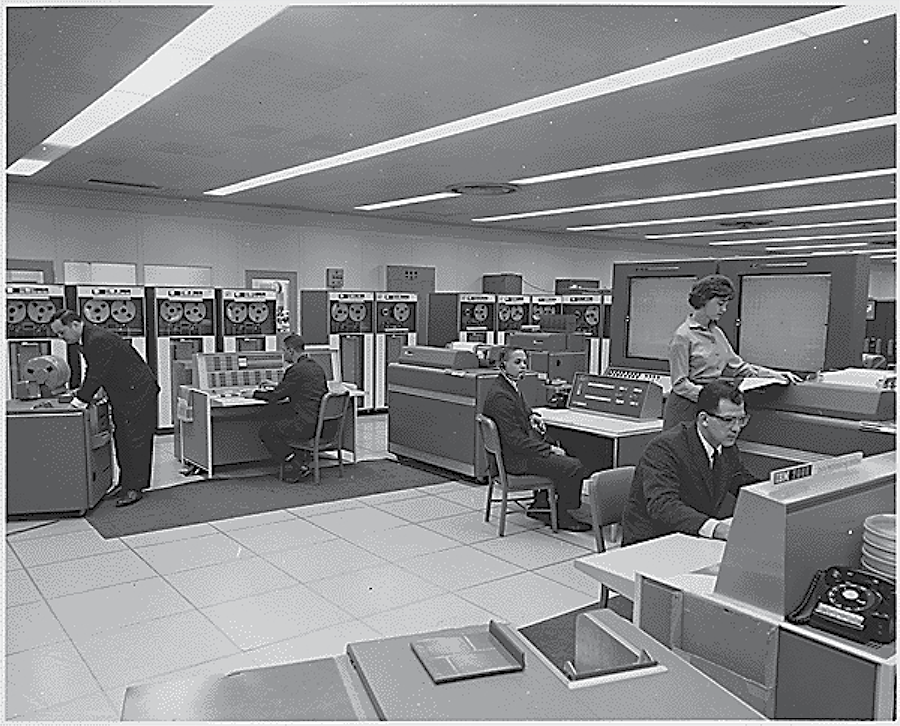
IBM 7094 mainframe. (From National Archives and Records Administration, record # 278195, author unknown, http://arcweb.archives.gov/arc/action/ExternalIdSearch?id=278195&jScript=true .)
During the 1950s, the silicon chip was introduced. By 1964, the first silicon chips were used in computers, ushering in the third generation. The chips, known as printed circuits or integrated circuits (ICs), could incorporate dozens of transistors. The IC would be a pattern of transistors etched onto the surface of a piece of silicon, which would conduct electricity, thus the term semiconductor. Pins would allow the IC, or chip, to be attached to a socket, so that electrical current could flow from one location in the computer through the circuit and out to another location. Figure 7.10 shows both the etchings that make up an IC and the chip itself with pins to insert the chip into a motherboard. The chip shown in Figure 7.10 is a typical chip from the late 1960s.
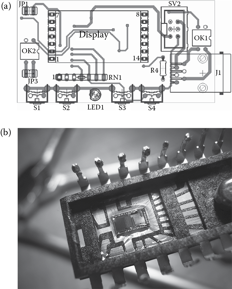
An integrated circuit (a) (Courtesy of Martin Broz, http://commons.wikimedia.org/wiki/File:Navrh_plosny_spoj_soucastky.png .) and a silicon chip (b) (Courtesy of Xoneca, http://commons.wikimedia.org/wiki/File:Integrated_circuit_optical_sensor.jpg .)
ICs would replace both the bulkier transistors and magnetic core memories, so that chips would be used for both computation and storage. ICs took up less space, so again the distance that current had to flow was reduced even more. Faster computers were the result. Additionally, ICs could be mass produced, so the cost of manufacturing a computer was reduced. Now, even small-sized organizations could consider purchasing a computer. Mainframe computers were still being produced at costs of perhaps $100,000 or more. Now, though, computer companies were also producing minicomputers at a reduced cost, perhaps as low as $16,000. The minicomputers were essentially scaled-down mainframes, they used the same type of processor, but had reduced number of registers and processing elements, reduced memory, reduced storage, and so forth, so that they would support fewer users. A mainframe might be used by a large organization of hundreds or thousands of people, whereas a minicomputer might be used by a small organization with tens or hundreds of users.
During the third generation, computer companies started producing families of computers. The idea was that any computer in a given family should be able to run the same programs without having to alter the program code. This was largely attributable to computers of the same family using the same processor, or at least processors that had the same instruction set (machine language). The computer family gave birth to the software development field as someone could write code for an entire family and sell that program to potentially dozens or hundreds of customers.
Organizations were now purchasing computers with the expectation that many employees (dozens, hundreds, even thousands) would use it. This created a need for some mechanisms whereby the employees could access the computer remotely without having to go to the computer room itself. Computer networks were introduced that would allow individual users to connect to the computer via dumb terminals (see Figure 7.11). The dumb terminal was merely an input and output device, it had no memory or processor. All computation and storage took place on the computer itself. Operating systems were improved to handle multiple users at a time. Operating system development is also described in Evolution of Computer Software.
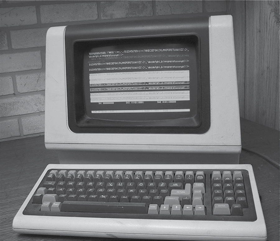
A dumb terminal, circa 1980. (Adapted from Wtshymanski, http://en.wikipedia.org/wiki/File:Televideo925Terminal.jpg .)
Fourth Generation
The next major innovation took place in 1974 when IBM produced a single-chip processor. Up until this point, all processors were distributed over several, perhaps dozens, of chips (or in earlier days, vacuum tubes and relay switches or transistors). By creating a single-chip processor, known as a microprocessor, one could build a small computer around the single chip. These computers were called microcomputers. Such a computer would be small enough to sit on a person’s desk. This ushered in the most recent generation, the fourth generation.
It was the innovation of the microprocessor that led to our first personal computers in the mid 1970s. These computers were little more than hobbyist devices with little to no business or personal capabilities. These early microcomputers were sold as component parts and the hobbyist would put the computer together, perhaps placing the components in a wooden box, and attaching the computer to a television set or printer. The earliest such computer was the Mark 8. Apple Computers was established in 1976, and their first computer, the Apple I, was also sold as a kit that people would build in a box. Unlike the Mark 8, the Apple I became an overnight sensation (Figure 7.12).
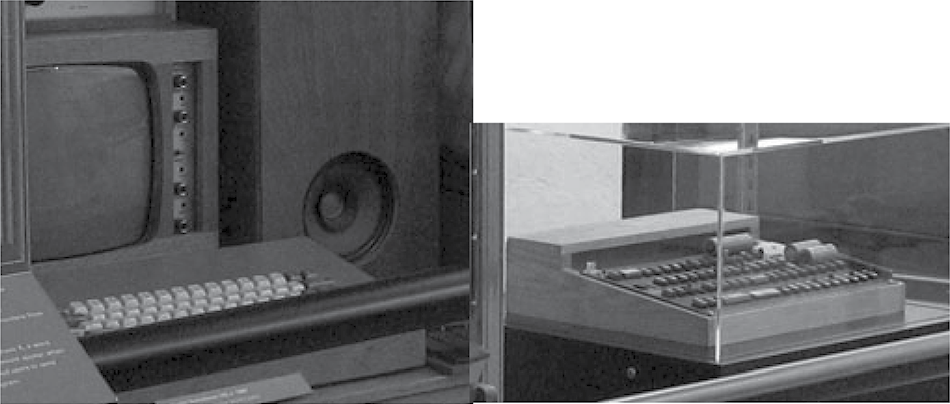
Apple I built in a wooden box. (Courtesy of Alpha1, http://commons.wikimedia.org/wiki/File:Apple_1_computer.jpg .)
Although the early microcomputers were of little computing use being hobbyist toys, over time they became more and more popular, and thus there was a vested interest in improving them. By the end of the 1970s, both microprocessors and computer memory capacities improved, allowing for more capable microcomputers—including those that could perform rudimentary computer graphics. Modest word processing and accounting software, introduced at the end of the 1970s, made these computers useful for small and mid-sized businesses. Later, software was introduced that could fill niche markets such as desktop publishing, music and arts, and education. Coupled with graphical user interfaces (GUI), personal computers became an attractive option not just for businesses but for home use. With the introduction of a commercialized Internet, the computer became more than a business or educational tool, and today it is of course as common in a household as a car.
The most significant change that has occurred since 1974 can be summarized in one word: miniaturization. The third-generation computers comprised multiple circuit boards, interconnected in a chassis. Each board contained numerous ICs and each IC would contain a few dozen transistors (up to a few hundred by the end of the 1960s). By the 1970s, it was possible to miniaturize thousands of transistors to be placed onto a single chip. As time went on, the trend of miniaturizing transistors continued at an exponential rate.
Most improvements in our society occur at a slow rate, at best offering a linear increase in performance. Table 7.2 demonstrates the difference between an exponential and a linear increase. The linear improvement in the figure increases by a factor of approximately 20% per time period. This results in a doubling of performance over the initial performance in about five time periods. The exponential improvement doubles each time period resulting in an increase that is orders-of-magnitude greater over the same period. In the table, an increase from 1000 to 128,000 occurs in just seven time periods.
Linear versus Exponential Increase
|
1000 |
1000 |
|
1200 |
2000 |
|
1400 |
4000 |
|
1600 |
8000 |
|
1800 |
16,000 |
|
2000 |
32,000 |
|
2200 |
64,000 |
|
2400 |
128,000 |
What does this mean with respect to our computers? It means that over the years, the number of transistors that can be placed on a chip has increased by orders of magnitude rather than linearly. The improvements in our computers have been dramatic in fairly short periods. It was Gordon Moore, one of the founders of Intel, who first noticed this rapidly increasing “transistor count” phenomenon. In a 1965 paper, Moore observed that the trend from 1958 to 1965 was that the number of transistors on a chip was doubling every year. This phenomenon has been dubbed “Moore’s law.” Moore predicted that this trend would continue for at least 10 more years.
We find, in fact, that the degree of miniaturization is a doubling of transistor count roughly every 18 to 24 months, and that this trend has continued from 1965 to the present. The graph in Figure 7.13 illustrates the progress made by noting the transistor count on a number of different processors released between 1971 and 2011. It should be reiterated that Moore’s law is an observation, not a physical law. We have come to rely on the trend in miniaturization, but there is certainly no guarantee that the trend will continue forever. In fact, there were many engineers who have felt that the rate of increase would have to slow down by 2000. Once we reached 2000 and Moore’s law continued to be realized, engineers felt that 2010 would see the end of this trend. Few engineers today feel that Moore’s law will continue for more than a few more years or a decade, and so there is a great deal of active research investigating new forms of semiconductor material other than silicon.
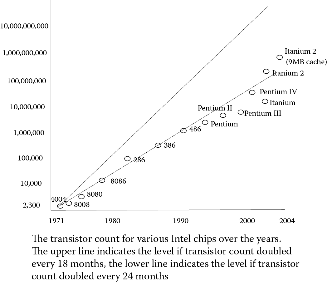
Charting miniaturization—Moore’s law. The scale on the left increases exponentially, not linearly. (Adapted from Wgsimon, http://commons.wikimedia.org/wiki/File:Moore_Law_diagram _%282004%29.jpg .)
What might it mean if Moore’s law was to fail us? Consider how often you purchase a car. Most likely, you buy a car because your current car is not road-worthy—perhaps due to accidents, wear and tear from excessive mileage, or failure to keep the car up to standards (although in some cases, people buy new cars to celebrate promotions and so forth). Now consider the computer. There is little wear and tear from usage and component parts seldom fail (the hard disk is the one device in the computer with moving parts and is likely to fail much sooner than any other). The desire to purchase a new computer is almost entirely made because of obsolescence.
What makes a computer obsolete? Because newer computers are better. How are they better? They are faster and have more memory. Why? Because miniaturization has led to a greater transistor count and therefore more capable components that are faster and have larger storage. If we are unable to continue to increase transistor count, the newer computers will be little better or no better than current computers. Therefore, people will have less need to buy a new computer every few years. We will get back to this thought later in the chapter.
Moore’s law alone has not led us to the tremendously powerful processors of today’s computers. Certainly, the reduction in size of the components on a chip means that the time it takes for the electrical current to travel continues to lessen, and so we gain a speedup in our processors. However, of greater importance are the architectural innovations to the processor, introduced by computer engineers. These have become available largely because there is more space on the chip itself to accommodate a greater number of circuits. Between the excessive amount of miniaturization and the architectural innovations, our processors are literally millions of times more powerful than those of the ENIAC. We also have main memory capacities of 8 GB, a number that would have been thought impossible as recently as the 1980s.
Many architectural innovations have been introduced over the years since the mid 1960s. But it is the period of the past 20 or so years that has seen the most significant advancements. One very important innovation is the pipelined CPU. In a pipeline, the fetch–execute cycle is performed in an overlapped fashion on several instructions. For instance, while instruction 1 is being executed, instruction 2 is being decoded and instruction 3 is being fetched. This would result in three instructions all being in some state of execution at the same time. The CPU does not execute all three simultaneously, but each instruction is undergoing a part of the fetch–execute cycle. Pipelines can vary in length from three stages as described here to well over a dozen (some of the modern processors have 20 or more stages). The pipelined CPU is much like an automotive assembly line. In the assembly line, multiple workers are working on different cars simultaneously.
Other innovations include parallel processing, on-chip cache memories, register windows, hardware that speculates over whether a branch should be taken, and most recently, multiple cores (multiple CPUs on a single chip). These are all concepts studied in computer science and computer engineering.
The impact of the microprocessor cannot be overstated. Without it, we would not have personal computers and therefore we would not have the even smaller computing devices (e.g., smart phones). However, the fourth generation has not been limited to just the innovations brought forth by miniaturization. We have also seen immense improvements in secondary storage devices. Hard disk capacity has reached and exceeded 1 TB (i.e., 1 trillion bytes into which you could store 1 billion books of text or about 10,000 high-quality CDs or more than 1000 low-resolution movies). Flash drives are also commonplace today and provide us with portability for transferring files. We have also seen the introduction of long-lasting batteries and LCD technologies to provide us with powerful laptop and notebook computers. Additionally, broadband wireless technology permits us to communicate practically anywhere.
Machines that Changed the World
In 1992, PBS aired a five-part series on the computer called The Machine That Changed the World. It should be obvious in reading this chapter that many machines have changed our world as our technology has progressed and evolved. Here is a list of other machines worth mentioning.
Z1—built by Konrad Zuse in Germany, it predated the ENIAC although was partially mechanical in nature, using telephone relays rather than vacuum tubes.
UNIVAC I—built by the creators of the ENIAC for Remington Rand, it was the first commercial computer, starting in 1951.
CDC 6600—the world’s first supercomputer was actually released in 1964, not the 1980s! This mainframe outperformed the next fastest computer by a factor of 3.
Altair 8800—although the Mark 8 was the first personal computer, it was the Altair 8800 that computer hobbyists initially took to. This computer was also sold as a computer kit to be assembled. Its popularity though was nothing compared to the Apple I, which followed 5 years later.
IBM 5100—the first commercially available laptop computer (known as a portable computer in those days). The machine weighed 53 lb and cost between $9000 and $19,000!
IBM Simon—In 1979, NTT (Nippon Telegraph and Telephone) launched the first cellular phones. But the first smart phone was the IBM Simon, released in 1992. Its capabilities were limited to mobile phone, pager, fax, and a few applications such as a calendar, address book, clock, calculator, notepad, and e-mail.
Today, we have handheld devices that are more powerful than computers from 10 to 15 years ago. Our desktop and laptop computers are millions of times more powerful than the earliest computers in the 1940s and 1950s. And yet, our computers cost us as little as a few hundred to a thousand dollars, little enough money that people will often discard their computers to buy new ones within just a few years’ time. This chapter began with a comparison of the car and the computer. We end this section with a look at some of the milestones in the automotive industry versus milestones in the computer industry (Table 7.3). Notice that milestones in improved automobiles has taken greater amounts of time than milestones in computing, whereas the milestones in the automobile, for the most part, have not delivered cars that are orders-of-magnitude greater as the improvements have in the computing industry.
Milestone Comparisons
|
Year |
Automotive Milestone |
Computing Milestone |
Year |
|
6500 b.c. |
The wheel |
Abacus |
4000? b.c. |
|
1769 |
Steam-powered vehicles |
Mechanical calculator |
1642 |
|
1885 |
Automobile invented |
Programmable device |
1801 |
|
1896 |
First automotive death (pedestrian hit by a car going 4 mph) |
First mechanical computer designed (analytical engine) |
1832 |
|
1904 |
First automatic transmission |
First digital, electronic, general purpose computer (ENIAC) |
1946 |
|
1908 |
Assembly line permits mass production |
Second-generation computers (cheaper, faster, more reliable) |
1959 |
|
1911 |
First electric ignition |
Third-generation computers (ICs, cheaper, faster, computer families) |
1963 |
|
1925 |
About 250 highways available in the United States |
ARPANET (initial incarnation of the Internet) |
1969 |
|
1940 |
One quarter of all Americans own a car |
Fourth-generation computers (microprocessors, PCs) |
1974 |
|
1951 |
Cars reach 100 mph at reasonable costs |
First hard disk for PC |
1980 |
|
1956 |
Interstate highway system authorized (took 35 years to complete) |
IBM PC released |
1981 |
|
1966 |
First antilock brakes |
Macintosh (first GUI) |
1984 |
|
1973 |
National speed limits set in the United States, energy crisis begins |
Stallman introduces GNUs |
1985 |
|
1977 |
Handicapped parking introduced |
Internet access in households |
1990s |
|
1997 |
First hybrid engine developed |
Cheap laptops, smart phones |
2000s |
Evolution of Computer Software
The earliest computers were programmed in machine language (recall from Chapter 2 that a machine language program is a lengthy list of 1s and 0s). It was the engineers, those building and maintaining the computers of the day, who were programming the computers. They were also the users, the only people who would run the programs. By the second generation, better programming languages were produced to make the programming task easier for the programmers. Programmers were often still engineers, although not necessarily the same engineers. In fact, programmers could be business people who wanted software to perform operations that their current software could not perform. In the mid 1960s, IBM personnel made a decision to stop producing their own software for their hardware families. The result was that the organizations that purchased IBM computers would have to go elsewhere to purchase software. Software houses were introduced and the software industry was born.
The history of software is not nearly as exhilarating as the history of hardware. However, over the decades, there have been a number of very important innovations. These are briefly discussed in this section. As IT majors, you will have to program, but you will most likely not have to worry about many of the concerns that arose during the evolution of software because your programs will mostly be short scripts. Nonetheless, this history gives an illustration of how we have arrived where we are with respect to programming.
Early computer programs were written in machine language, written for a specific machine, often by the engineers who built and ran the computers themselves. Entering the program was not a simple matter of typing it in but of connecting memory locations to computational circuits by means of cable, much like a telephone operator used to connect calls. Once the program was executed, one would have to “rewire” the entire computer to run the next program. Recall that early computers were unreliable in part because of the short lifetime and unreliability of vacuum tubes. But add to that the difficult nature of machine language programming and the method of entering the program (through cables), and you have a very challenging situation. As a historical note, an early programmer could not get his program working even though the vacuum tubes were working, his logic was correct, and the program was correctly entered. It turned out that a moth had somehow gotten into a relay switch so that it would not pass current. This, supposedly, has led to the term bug being used to mean an error. We now use the term debugging not only to refer to removal of errors in a program, but just about any form of troubleshooting! See Figure 7.14.
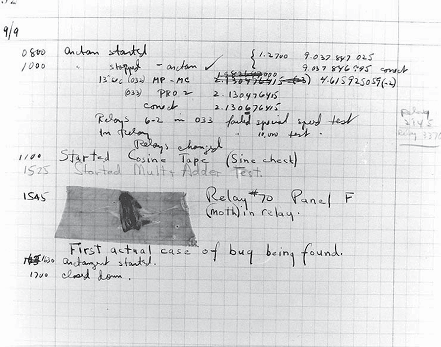
The first computer bug. (Courtesy of the U.S. Naval Historical Center, Online library photograph NH 96566-KN.)
Recall at this time, that computer input/output (I/O) was limited mostly to reading from punch cards or magnetic tape and writing to magnetic tape. Any output produced would be stored onto tape, unmounted from the tape drive, mounted to a printer, and then printed out. Since a computer only ran one program at a time and all input and output was restricted in such a manner, there was no need for an operating system for the computer. The programmer would include any I/O-specific code in the program itself.
The programming chore was made far easier with several innovations. The first was the idea of a language translator program. This program would take another program as input and output a machine language version, which could then be run on the computer. The original program, often known as the source code, could not be executed in its original form. The earliest language translators were known as assemblers, which would translate an assembly program into machine language. Assembly language, although easier than machine language, still required extremely detailed, precise, and low-level instructions (recall the example from Chapter 2). By 1959, language translation improved to the point that the language converted could be written in a more English-like way with far more powerful programming constructs. The improved class of language translator was known as a compiler, and the languages were called high-level languages. The first of these language translators was made for a language called FORTRAN. The idea behind FORTRAN was that the programmer would largely specify mathematical formulas using algebraic notation, along with input, output, and control statements. The control statements (loops, selections) would be fairly similar to assembly language, but the rest of the language would read more like English and mathematics. The name of the language comes from FORmula TRANslator. FORTRAN was primarily intended for mathematic/scientific computing. A business-oriented language was also produced at roughly the same time called COBOL (Common Business Oriented Language). Other languages were developed to support artificial intelligence research (LISP), simulation (Simula), and string manipulations (SNOBOL).
Let us compare high level code to that of assembly and machine language. Figure 7.15 provides a simple C statement that computes the summation of all integer values from 1 to an input value, x. The C code is a single statement: a for loop. The for loop’s body is itself a single assignment statement.
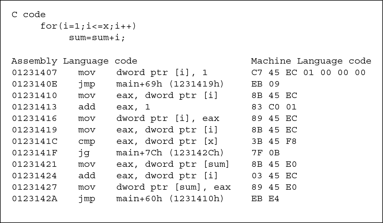
When this single C instruction is assembled into assembly language code (for the Intel x86 processor), the code is 12 instructions long. This is shown in the figure as three columns of information. The first column contains the memory address storing the instruction. The second column is the actual operation, represented as a mnemonic (an abbreviation). The third column contains the operands (data) that the instruction operates on.
For instance, the first instruction moves the value 1 into the location pointed to by a variable referenced as dword ptr. The fourth instruction is perhaps the easiest to understand, add eax, 1 adds the value 1 to the data register named the eax. Each assembly instruction is converted into one machine language instruction. In this case, the machine language (on the right-hand side of the figure) instructions are shown in hexadecimal. So, for instance, the first mov instruction (data movement) consists of 14 hexadecimal values, shown in pairs. One only need examine this simple C code to realize how cryptic assembly language can be. The assembly language mnemonics may give a hint as to what each operation does, but the machine language code is almost entirely opaque to understanding. The C code instead communicates to us with English words like for, along with variables and mathematical notation.
Programmers Wanted!
Computer scientist and software engineer are fairly recent terms in our society. The first computer science department at a university was at Purdue University in 1962. The first Ph.D. in Computer Science was granted from the University of Pennsylvania in 1965. It was not until the 1970s that computer science was found in many universities. Software engineering was not even a term in our language until 1968.
Today, most programmers receive computer science degrees although there are also some software engineering degree programs. But who were the programmers before there were computer scientists? Ironically, like the story of Joe from Chapter 1, the computer scientist turned IT specialist, early programmers were those who learned to program on their own. They were engineers and mathematicians, or they were business administrators and accountants. If you knew how to program, you could switch careers and be a computer programmer.
Today, computer programmer is a dying breed. Few companies are interested in hiring someone who knows how to program but does not have a formal background in computing. So, today, when you see programming in a job listing, it will most likely require a computer science, information systems, computer engineering, or IT degree.
Although assembly language is not impossible to decipher for a programmer, it is still a challenge to make sense of. High level language code, no matter which language, consists of English words, mathematical notation, and familiar syntax such as a semicolon used to end statements. The C programming language was not written until 1968; however, the other high level languages of that era (FORTRAN, COBOL, etc.) were all much easier to understand than either machine or assembly language. The move to high level programming languages represents one of the more significant advances in computing because without it, developing software would not only be a challenge, the crude programming languages would restrict the size of the software being developed. It is unlikely that a team of 20 programmers could produce a million-line program if they were forced to write in either machine or assembly language.
Into the 1960s, computers were becoming more readily available. In addition, more I/O resources were being utilized and computer networks were allowing users to connect to the computer from dumb terminals or remote locations. And now, it was not just the engineers who were using and programming computers. In an organization that had a computer, any employee could wind up being a computer user. These users might not have understood the hardware of the computer, nor how to program the computer. With all of these added complications, a program was required that could allow the user to enter simple commands to run programs and move data files in such a way that the user would not have to actually write full programs. This led to the first operating systems.
In the early 1960s, the operating system was called a resident monitor. It would always be resident in memory, available to be called upon by any user. It was known as a monitor because it would monitor user requests. The requests were largely limited to running a program, specifying the location of the input (which tape drive or disk drive, which file(s)), and the destination of the output (printer, disk file, tape file, etc.). However, as the 1960s progressed and more users were able to access computers, the resident monitor had to become more sophisticated. By the mid 1960s, the resident monitor was being called an operating system—a program that allowed a user to operate the computer. The operating system would be responsible for program scheduling (since multiple programs could be requested by several users), program execution (starting and monitoring the program during execution, terminating the program when done), and user interface. The operating system would have to handle the requests of multiple users at a time. Program execution was performed by multiprogramming at first, and later on, time sharing (now called multitasking).
Operating systems also handled user protection (ensuring that one user does not violate resources owned by another user) and network security. Throughout the 1960s and 1970s, operating systems were text-based. Thus, even though the user did not have to understand the hardware or be able to program a computer, the user was required to understand how to use the operating system commands. In systems such as VMS (Virtual Memory System) run on DEC (Digital Equipment Corporation) VAX computers and JCL (Job Control Language) run on IBM mainframes, commands could be as elaborate and complex as with a programming language.
With the development of the personal computer, a simpler operating system could be applied. One of the most popular was that of MS-DOS, the disk operating system. Commands were largely limited to disk (or storage) operations—starting a program, saving a file, moving a file, deleting a file, creating directories, and so forth. Ironically, although the name of the operating system is DOS, it could be used for either disk or tape storage! The next innovation in operating systems did not arise until the 1980s. However, in the meantime….
Lessons learned by programmers in the 1960s led to a new revolution in the 1970s known as structured programming. Statements known as GOTOs were used in a large number of early languages. The GOTO statement allowed the programmer to transfer control from any location in a program to anywhere else in the program. For a programmer, this freedom could be a wonderful thing—until you had to understand the program to modify it or fix errors. The reason is that the GOTO statement creates what is now called spaghetti code. If you were to trace through a program, you would follow the instructions in sequential order. However, with the use of GOTO statements, suddenly after any instruction, you might have to move to another location in the program. Tracing through the program begins to look like a pile of spaghetti. In structured programming, the programmer is limited to high level control constructs such as while loops, for loops, and if–else statements, and is not allowed to use the more primitive GOTO statement. This ushered in a new era of high level languages, C and Pascal being among the most notable.
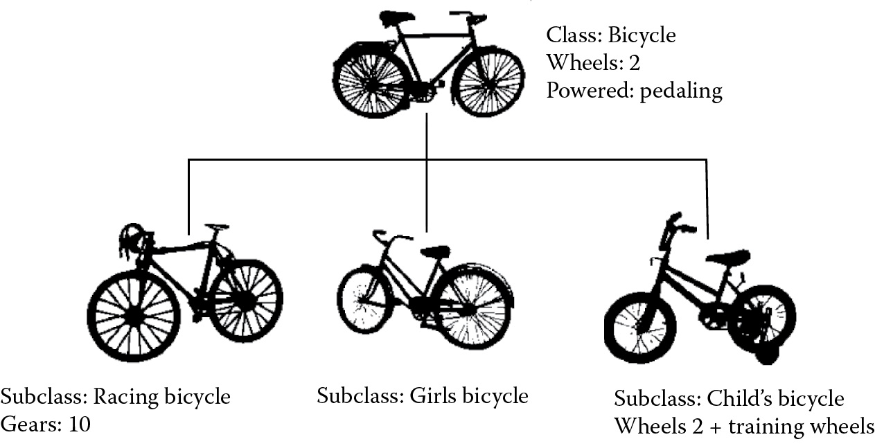
In the 1980s, another innovation looked to rock the programming world. Up until the mid 1980s, a programmer who wanted to model some entity in the world, whether a physical object such as a car, or an abstract object such as a word process document, would use individual variables. The variables would describe attributes of the object. For the car, for instance, variables might include age, gas mileage, type of car, number of miles, and current Blue Book value. A better modeling approach was to define classes of entities called objects. Objects could then be spawned by a program, each object being unique and modeling a different physical object (for instance, given a car class, we could generate four different cars). Objects would then interact with each other and with other types of objects. The difference between the object-oriented approach and the older, variable-based approach, is that an object is a stand-alone entity that would be programmed to handle its own internal methods as well as messages received from other objects. And with classes defined, a programmer could then expand the language by defining child classes. Through a technique called inheritance, a programmer is able to take a previous class and generate a more specific class out of it. This provides a degree of code reuse in that programmers could use other programmers’ classes without having to reinvent the code themselves. The notion of inheritance is illustrated in Figure 7.16, where a bicycle class is the basis for several more specific types of bicycles. For instance, all bicycles in the hierarchy represent modes of transportation that contain two wheels powered by a human pedaling. However, there are subtypes of bicycles such as a racing bike, a girl’s bike, or a bike with training wheels.
Object-oriented programming (OOP) was initially introduced in the language Smalltalk in the 1970s and early 1980s. In the mid 1980s, a variant of Smalltalk’s object-oriented capabilities was incorporated into a new version of C, called C++. C++ became so popular that other object-oriented programming languages (OOPL) were introduced in the 1990s. Today, nearly every programming language has OOP capabilities.
Hand in hand with the development of OOPLs was the introduction of the first windowing operating system. To demonstrate the use of OOP, artificial intelligence researchers at Xerox Palo Alto California (Xerox Parc) constructed a windows-based environment. The idea was that a window would be modeled as an object. Every window would have certain features in common (size, location, background color) and operations that would work on any window (moving it, resizing it, collapsing it). The result was a windows operating system that they would use to help enhance their research. They did not think much of marketing their creation, but they were eager to demonstrate it to visitors. Two such visitors, Steven Jobs and Steven Wozniak (the inventors of the Apple personal computers), found this innovation to be extraordinary and predicted it could change computing. Jobs and Wozniak spent many years implementing their own version. Jobs was involved in the first personal computer to have the GUI, the Apple Lisa. But when it was released in 1983 for $10,000 per unit, very few were sold. In fact, the Lisa project became such a mess that Jobs was forced off of the project in 1982 and instead, he moved onto another Apple project, the Macintosh. Released in 1984 for $2500, the Macintosh was a tremendous success.†
A windows-based interface permits people to use a computer by directing a pointer at menu items or using clicking and dragging motions. With a windowing system, one does not need to learn the language of an operating system such as VMS, DOS, or Unix, but instead, one can now control a computer intuitively after little to no lessons. Thus, it was the GUI that opened up computer usage to just about everyone. Today, graphical programming and OOP are powerful tools for the programmer. Nearly all software today is graphical in nature, and a good deal of software produced comes from an object-oriented language.
Another innovation in programming is the use of an interpreter rather than a compiler. The compiler requires that the components of the software all be defined before compilation can begin. This can be challenging when a software project consists of dozens to hundreds of individual components, all of which need to be written before compilation. In a language such as Java, for instance, one must first write any classes that will be called upon by another class. However, if you simply want to test out an idea, you cannot do so with incomplete code. The Lisp programming language, developed at the end of the 1950s for artificial intelligence research, used an interpreter. This allowed programmers to test out one instruction at a time, so that they could build their program piecemeal.
The main difference between a compiled language and an interpreted language is that the interpreted language runs inside of a special environment called the interpreter. The programmer enters a command, then the interpreter converts that command to machine language and executes it. The command might apply the result of previous commands by referring to variables set by earlier commands, although it does not necessarily have to. Thus, interpreted programming relies on the notion of a session. If the programmer succeeds in executing several instructions that go together, then the programmer can wrap them up into a program. In the compiled language, the entire program is written before it can be compiled, which is necessary before it can be executed. There are many reasons to enjoy the interpreted approach to programming; however, producing efficient code is not one of them. Therefore, most large software projects are compiled.
As an IT administrator, your job will most likely require that you write your own code from time to time. Fortunately, since efficiency will not necessarily be a concern (your code will be relatively small, perhaps as few as a couple of instructions per program), you can use an interpreted environment. In the Linux operating system, the shell contains its own interpreter. Therefore, writing a program is a matter of placing your Linux commands into a file. These small programs are referred to as scripts, and the process of programming is called shell scripting. In Windows, you can write DOS batch files for similar results.
Scripting goes beyond system administration, however. Small scripts are often written in network administration, web server administration, and database server administration. Scripts are also the tool of choice for web developers, who will write small scripts to run on the web server (server-side scripts), or in the web browser (client-side scripts). Server-side scripts, for instance, are used to process data entered in web-page forms or for generating dynamic web pages by pulling information out of a database. Client-side scripts are used to interact with the user, for instance, by ensuring that a form was filled out correctly or through a computer game. Many of the interpreted languages today can serve as scripting languages for these purposes. Scripting languages include perl, php, ruby, python, and asp. We will visit programming and some of these scripting languages in more detail in Chapter 14.
Evolution of the Computer User
Just as computer hardware and computer software have evolved, so has the computer user. The earliest computer users were the engineers who both built and programmed the computers. These users had highly specialized knowledge of electronics, electrical engineering, and mathematics. There were only hundreds of such people working on a few dozen laboratory machines. By the 1950s, users had progressed to include programmers who were no longer (necessarily) the engineers building the computers.
In the 1960s and through the 1970s, users included the employees of organizations that owned or purchased time on computers. These users were typically highly educated, but perhaps not computer scientists or engineers. Some of the users were computer operators, whose job included such tasks as mounting tapes on tape drives and working with the computer hardware in clean rooms. But most users instead worked from their offices on dumb terminals. For this group of users, their skills did not have to include mathematics and electronics, nor programming, although in most cases, they were trained on the operating system commands of their computer systems so that they could enter operating system instructions to accomplish their tasks. The following are some examples from VMS, the operating system for DEC’s VAX computers, which were very popular in the 1970s and 1980s (excerpted from a tutorial on VMS).
ASSIGN DEV$DISK:[BOB]POSFILE.DAT FOR015
COPY SYS$EXAMPLES:TUT.FOR TUT.FOR
DEL SYS$EXAMPLES:TUT.FOR
PRINT/FORM = 1/QUEUE = SYS$LASER TUT.FOR
SHOW QUEUE/ALL SYS$LASER
As the 1970s progressed, the personal computer let just about anyone use a computer regardless of their background. To control the early PCs, users had to know something of the operating system, so again, they wrote commands. You have already explored some MS-DOS commands earlier in the text. Although the commands may not be easy to remember, there are far fewer commands to master than in the more complex mainframe operating systems such as VMS.
With the release of the Apple Macintosh in 1984, however, the use of operating system commands became obsolete. Rather than entering cryptic commands at a prompt, the user instead controlled the computer using the GUI. All of the Macintosh software was GUI-based such that, for the first time, a user would not have to have any specialized knowledge to use the computer. It was intuitively easy. The Microsoft Windows operating system was introduced a year later, and by the 1990s, nearly all computers were accessible by windows-based GUI operating systems and applications software. In an interesting turn of events, it was often the younger generations who easily learned how to use the computer, whereas the older generations, those who grew up thinking that computers were enormous, expensive, and scary, were most hesitant to learn to use computers.
The most recent developments in computer usage is the look and feel of touch screen input devices such as smart phones and tablet PCs. Pioneered by various Apple products, the touch screen provides an even more intuitive control of the computer over the more traditional windows-style GUI. Scrolling, tapping, bringing up a keyboard, and using your fingers to move around perhaps is the next generation of operating systems. It has already been announced that Microsoft plans on adopting this look and feel to their next generation of desktop operating system, Windows 8.
Today, it is surprising to find someone who does not know how to use a computer. The required skill level remains low for using a computer. In fact, with so many smart phones on the planet, roughly half of the population of the planet can be considered computer users.
To understand computer fundamentals, one must know some basic computer literacy. To understand more advanced concepts such as software installation, hardware installation, performance monitoring, and so forth, even greater knowledge is needed. Much of this knowledge can be learned by reading manuals or magazines. It can also be learned by watching a friend or family member do something similar. Some users learn by trial and error. Today, because of the enormous impact that computers have had on our society, much of this knowledge is easily accessible over the Internet as there are web sites that both computer companies and individuals create that help users learn. Only the most specialized knowledge of hardware repair, system/network administration, software engineering, and computer engineering require training and/or school.
Impact on Society
You are in your car, driving down the street. You reach a stop light and wait for it to change. Your GPS indicates that you should go straight. You are listening to satellite radio. While at the stop light, you are texting a friend on your smart phone (now illegal in some states). You are on your way to the movies. Earlier, you watched the weather forecast on television, telling you that rain was imminent. While you have not touched your computer today, you are immersed in computer technology.
- Your car contains several processors: the fuel-injection carburetor, the antilock brakes, the dashboard—these are all programmable devices with ICs.
- Your GPS is a programmable device that receives input from a touch screen and from orbiting satellites.
- Your satellite radio works because of satellites in orbit, launched by rocket and computer, and programmed to deliver signals to specific areas of the country.
- Your smart phone is a scaled-down computer.
- The movie you are going to see was written almost certainly by people using word processors. The film was probably edited digitally. Special effects were likely added through computer graphics. The list of how computers were used in the production of the film would most likely be lengthy, and that does not take into account marketing or advertising of the movie.
- The weather was predicted thanks to satellites (again, placed in orbit by rocket and computer), and the weather models were run on computers.
- Even the stop light is probably controlled by a computer. See the sensors in the road?
In our world today, it is nearly impossible to escape interaction with a computer. You would have to move to a remote area and purposefully rid yourself of the technology in order to remove computers from your life. And yet you may still feel their impact through bills, the post office, going to country stores, and from your neighbors.
Computer usage is found in any and every career. From A to Z, whether it be accounting, advertising, air travel, the armed forces, art, or zoology, computers are used to assist us and even do a lot of the work for us.
But the impact is not limited to our use of computers in the workforce. They are the very basis for economic transactions. Nearly all of our shopping takes place electronically: inventory, charging credit cards, accounting. Computers dominate our forms of entertainment whether it is the creation of film, television programs, music, or art, or the medium by which we view/listen/see the art. Even more significantly, computers are now the center of our communications. Aside from the obvious use of the cell phone for phone calls, we use our mobile devices to see each other, to keep track of where people are (yes, even spy on each other), to read the latest news, even play games.
And then there is the Internet. Through the Internet, we shop, we invest, we learn, we read (and view) the news, we seek entertainment, we maintain contact with family, friends, and strangers. The global nature of the Internet combined with the accessibility that people have in today’s society has made it possible for anyone and everyone to have a voice. Blogs and posting boards find everyone wanting to share their opinions. Social networking has allowed us to maintain friendships remotely and even make new friends and lovers.
The Internet also provides cross-cultural contact. Now we can see what it’s like to live in other countries. We are able to view those countries histories and historic sites. We can watch gatherings or entertainment produced from those countries via YouTube. And with social networking, we can find out, nearly instantaneously what news is taking place in those countries. As a prime example, throughout 2011, the Arab Spring was taking place. And while it unfolded, the whole world watched.
To see the impact of the computer, consider the following questions:
- When was the last time you wrote someone a postal letter? For what reason other than sending a holiday card or payment?
- When was the last time you visited a friend without first phoning them up on your cell phone or e-mailing them?
- When was the last time you read news solely by newspaper?
You will study the history of operating systems, with particular emphasis on DOS, Windows, and Linux, and the history of the Internet in Chapters 8 and 12, respectively. We revisit programming languages and some of their evolution in Chapter 14.
Further Reading
There are a number of excellent sources that cover aspects of computing from computer history to the changing social impact of computers. To provide a complete list could quite possibly be as lengthy as this text. Here, we spotlight a few of the more interesting or seminal works on the topic.
- Campbell-Kelly, M. and Aspray, W. Computer: A History of the Information Machine. Boulder, CO: Westview Press, 2004.
- Campbell-Kelly, M. From Airline Reservations to Sonic the Hedgehog: A History of the Software Industry. Cambridge, MA: MIT Press, 2004.
- Ceruzzi, P. A History of Modern Computing. Cambridge, MA: MIT Press, 1998.
- Ceruzzi, P. Computing: A Concise History. Cambridge, MA: MIT Press, 2012.
- Daylight, E., Wirth, N. Hoare, T., Liskov, B., Naur, P. (authors) and De Grave, K. (editor). The Dawn of Software Engineering: from Turing to Dijkstra. Heverlee, Belgium: Lonely Scholar, 2012.
- Ifrah, G. The Universal History of Numbers: From Prehistory to the Invention of the Computer. New Jersey: Wiley and Sons, 2000.
- Mens, T. and Demeyer, S. (editors). Software Evolution. New York: Springer, 2010.
- Rojas, R. and Hashagen, U. (editors). The First Computers: History and Architectures. Cambridge: MA: MIT Press, 2000.
- Stern, N. From ENIAC to UNIVAC: An Appraisal of the Eckert–Mauchly Computers. Florida: Digital Press, 1981.
- Swedin, E. and Ferro, D. Computers: The Life Story of a Technology. Baltimore, MD: Johns Hopkins University Press, 2007.
- Williams, M. History of Computing Technology. Los Alamitos, CA: IEEE Computer Society, 1997.
There are a number of websites dedicated to aspects of computer history. A few are mentioned here.
- http://americanhistory.si.edu/collections/comphist/
- http://en.wikipedia.org/wiki/Index_of_history_of_computing_articles
- http://www.computerhistory.org/
- http://www.computerhope.com/history/
- http://www.computersciencelab.com/ComputerHistory/History.htm
- http://www.trailing-edge.com/~bobbemer/HISTORY.HTM
Review terms
Terminology introduced in this chapter:
Abacus Compiler
Analytical Engine Difference Engine
Assembler Dumb terminal
Bug ENIAC
GUI Minicomputer
Integrated circuit OOPL
Interpreter Relay switch
Magnetic core memory Resident monitor
Mainframe Structured programming
Mechanical calculator Vacuum tube
Microcomputers Windows operating system
Microprocessor
Review Questions
- How did Pascal’s calculator actually compute? What was used to store information?
- What device is considered to be the world’s first programmable device?
- In what way(s) should we consider Babbage’s Analytical Engine to be a computer?
- What notable achievement did Lady Ada Augusta Lovelace have?
- Which of the four computer generations lasted the longest?
- In each generation, the hardware of the processor was reduced in size. Why did this result in a speed up?
- What was the drawback with using vacuum tubes?
- What technology replaced vacuum tubes for second generation computers?
- At what point in time did we see a shift in users from those who were building and programming computers to ordinary end users?
- Since both the third- and fourth-generation computers used integrated circuits on silicon chips, how did the hardware of the fourth generation differ from that of the third?
- In the evolution of operating systems, what was the most significant change that occurred in the fourth generation?
- In the evolution of operating systems, at what point did they progress from tackling one program at a time to switching off between multiple programs?
- What is structured programming and what type of programming instruction did structured programming attempt to make obsolete?
- How did object-oriented programming improve on programming?
- How do computer users today differ from those who used computers in the 1960s? From those who used computers in the 1950s?
Discussion Questions
- In your own words, describe the improvements in computer hardware in terms of size, expense, speed, value (to individuals), and cost from the 1950s to today.
- A comparison was made in this chapter that said “if cars had progressed like computers, …” Provide a similar comparison in terms of if medicine had progressed like computers.
- What other human achievements might rival that of the computer in terms of its progress and/or its impact on humanity?
- We might look at language as having an equal or greater impact on humanity as computers. Explain in what ways language impacts us more significantly than computer usage. Are there ways that computer usage impacts us more significantly than language?
- Provide a ranking of the following innovations, creations, or discoveries in terms of the impact that you see on our daily lives: fire, refrigeration, automobiles, flight, radio/television, computers (including the Internet).
- Imagine that a 50-year-old person has been stranded on an island since 1980 (the person would have been 18 at that time). How would you explain first what a personal computer is and second the impact that the personal computer has had on society?
- Describe your daily interactions with computers or devices that have computer components in them. What fraction of your day is spent using or interacting with these devices (including computers).
- Attempt to describe how your life would be different without the Internet.
- Attempt to describe how your life would be different without the cell phone.
- Attempt to describe how your life would be different without any form of computer (these would include your answers to questions #8 and #9).
- Imagine that computing is similar to how it was in the early 1980s. Personal computers were available, but most people either used them at home for simple bookkeeping tasks (e.g., accounting, taxes), word processing, and/or computer games, and businesses used them largely for specific business purposes such as inventory and maintaining client data. Furthermore, these computers were entirely or primarily text-based and not connected to the Internet. Given that state, would you be as interested in IT as a career or hobby? Explain.
* As with most discoveries in mathematics, Boole’s work was a continuation of other mathematicians’ work on logic including William Stanley Jevons, Augustus De Morgan, and Charles Sanders Peirce.
† For those of you old enough, you might recall the first Apple Macintosh commercial. Airing during Super Bowl XVIII in January 1984 for $1.5 million, the commercial showed a number of similarly dressed men walking through drab hallways and seated in an auditorium. They were listening to a “Big Brother”-like figure. A young female athlete in a white tank top ran into the hall and threw a hammer at the screen. Upon impact, the screen exploded and the commercial ended with the caption that “…you’ll see why 1984 won’t be like ‘1984.’ ” The commercial was directed by Ridley Scott. You can find the commercial on YouTube.