
Chapter 6
Reinsurance and Extremal Events
Eric Gilleland
Research Application Laboratory, National Center for Atmospheric Research Boulder, Colorado, USA
Mathieu Ribatet
Department of Mathematics, University of Montpellier Montpellier, France
6.1 Introduction
In risk analysis and especially for insurance applications, it is important to anticipate the losses that a given company might face in the near future. From a statistical point of view, the observed losses are assumed to be independent realizations from a non-negative random variable X whose distribution function is F.
In this chapter we will focus only on the largest losses, that is, the ones impacting the company's solvency. That is, we restrict our attention to the (right) tail of X. The theory related to the modeling of the tail of a distribution is known as extreme value theory and is widely applied in several domains such as finance, insurance, or risk analysis of natural hazards.
Contrary to inferences pertaining to averages of a random variable where larger values may be considered as outliers, and are often removed from the data, when considering extremes, it is the bulk of the data that are discarded, and the outliers that are of interest. Typically, therefore, one is left with a paucity of data for analyzing the extremes.
6.2 Univariate Extremes
Let X1,X2,... be independent copies of a random variable X with distribution F. If one is interested in modeling the (right) tail of X, different modeling strategies are possible:
- Analyzing block maxima, that is, characterizing the distribution of
Mn=max{X1,...,Xn},(6.1)
for some suitable large n∈ℕ;
- Looking at exceedances, that is, characterizing the distribution of
X |{X>u},(6.2)
for some suitable high threshold u∈ℝ.
Remark 6.1 When interest is in the minima or deficits below a low threshold, the same theory applies after making a suitable transformation (e.g.,min{X1,...,Xn}=−max{−X1,...,−Xn}).
The left panel of Figure 6.1 shows the 2,167 fire losses collected by Copenhagen Reinsurance between 1980 and 1990. It is clear that the exceedances approach makes more efficient use of the data because, contrary to the annual maxima, several exceedances might occur in a given year. However, this approach may induce serial dependence between excesses if the initial assumption of mutual independence of losses is wrong. This is usually not a problem with the block maxima methodology provided that the starting and closing times for the blocks have been defined with caution.

The left panel shows the time series of the Danish reinsurance claim dataset danishuni from the CASdatasets package. The two right-most panels illustrate the block maxima and exceedances approaches for modeling large losses. The claims are in millions of Danish Kroner and cover the time period 1980-1990.
6.2.1 Block Maxima
Because the Xi are independent and identically distributed, it is clear that ℙ(Mn≤x)=F(x)n. Unfortunately, for practical purposes, this result is of little interest because typically F has to be estimated, and a small error made on the estimation of F can have catastrophic consequences on the estimation of large quantiles of Mn. . Similar to the use of the normal distribution appearing in the central limit theorem, the strategy consists of using asymptotic results and we are therefore interested in characterizing the limiting distribution G such that
Mn−bnand→ G, n→∞,(6.3)
for some sequences of constants an>0 and bn∈ℝ.
The Fisher-Tippett theorem (see Embrechts et al. (1997), Section 3.3; Coles (2001), Theorem 3.3; or Beirlant et al. (2004), Theorem 2.1) states that, provided G is nondegenerate, there exist constants a>0 and b∈ℝ. such that G(ax+b)=Gξ(x), where
Gξ(x)=exp{−(1+ξx)−1/ξ}, 1+ξx>0,(6.4)
where ξ≠0. As ξ→0,Gξ is prolonged by continuity to give
Go(x)=exp{−exp(−x)},x∈ℝ.
The parameter ξ is known as the extreme value index and plays a major role in the behavior of the tail of X. When ξ<0, , G is upper bounded by −1/ξ and is said to be short tailed. When ξ=0, , G corresponds to the standard Gumbel distribution and is said to be light tailed (i.e., decays exponentially). When ξ>0 , H is lower bounded by −1/ξ and is said to be heavy tailed (i.e., decays geometrically). The limiting distribution is the Fréchet distribution with parameter 1/ξ.
For statistical purposes, (6.3) justifies the use of the class of distributions generated by (6.4) as a suitable class of distributions for modeling sample maxima. More precisely, we suppose that the asymptotic result in (6.3) is (approximately) met for finite but large enough n∈ℕ, that is,
P(Mn≤x)≈exp{−(1+ξx−μσ)−1/ξ}, 1+ξx−μσ>0,(6.5)
for some unknown location μ∈ℝ, , scale σ>0 and shape ξ≠0 parameters.
The distribution (6.5) is known as the generalized extreme value distribution and takes the Gumbel distribution as a special case when ξ→0, giving
P(Mn≤x)≈exp{−exp(−x−μσ)},x∈R.(6.6)
Figure 6.2 plots the probability density function of a generalized extreme value distribution with different shape parametersξ

Plot of generalized extreme value probability density functions with μ=σ=1 and, from left to right, ξ=0.5 ,0, —0.5.
The parameters μ and σ are required to embed both the unknown normalizing constants an and bn in (6.3) and the scaling constants a and b in the expression G(ax+b)=Gξ(x). A fundamental property of the block maxima approach is the max-stable property. A random variable Y is said to be max-stable if there exist constants cn>0 and dn∈ℝ such that
max{Y1,...,Yn}−dncnd__Y,(6.7)
for all n∈ℕ and where Y1,...,Yn are independent copies of Y. Loosely speaking, the max- stability property states that, up to a shift and scale transformation, the random variable Y is stable by the maximum operator and is similar to what the a-stability is for the addition operator (see Section 3.3 in Embrechts et al. (1997)).
It is straightforward to show that the generalized extreme value distribution at the righthand side of (6.5) is max-stable with
cn=nξ,dn=(1−cn)(μ−σξ).
Less formally, the max-stability property is desirable because for all n,k∈ℕ , we have
{X1,...,Xnk}=max{max(X1,...,Xn),...,max(Xn(k−1)+1,...,Xnk)} ,
that is, the “overall maximum” can be thought of as the maxima of several “sub-maxima.” Now as n→∞, both the overall maximum and these sub-maxima converge to (different) generalized extreme value distributions—under linear normalizations. The difference between the two limiting generalized extreme value distributions coming from the normalizing constants cn>0 and dn∈R in (6.7).
The following R code show how it is possible to retrieve the annual maxima from the Danish claim dataset.
> danish.claim <- danishuni[,2]
> years <- as.numeric(substr(danishuni[,1], 1, 4))
> danish.max <- aggregate(danish.claim, by=list(years), max,
+ na.rm=TRUE)[,2]
6.2.2 Exceedances above a Threshold
As illustrated by Figure 6.1, the threshold excess approach makes better, more efficient use of the available data by including all of the extreme values regardless of whether they
happen within some arbitrarily chosen block or not; with the potential issue of introducing dependence among those exceedances.
Because our interest is in the tail of X and we aim to derive asymptotic distributions for extreme events, it makes sense to characterize the limiting distribution H,
x−ua(u)|{X>u}d→H, u→x+,(6.8)
for some positive function a(.) and where x+=sup{x∈ℝ:F(x)<1}. Provided the limiting distribution G in (6.3) is nondegenerate, the Pickands-Balkema- de Haan theorem (see Embrechts et al. (1997), Section 3.4; Coles (2001), Theorem 4.2; or Beirlant et al. (2004), Section 4.5) states that there exists a>0 such that H(ax)=Hξ(x), where
Hξ(x)=1−(1+ξx)−1/ξ,1+ξx>0,(6.9)
where ξ≠0. Again, as ξ→0, Hξ is prolonged by continuity to give the exponential distribution
H0(x)=1−exp(−x), x>0.
The shape parameter ξ appearing in Hξ is the same as the one arising in the generalized extreme value distribution (6.4).
For statistical purposes, (6.8) justifies the use of the distributions generated by (6.9) to model excesses above a threshold and similarly to the reasoning made for block maxima, we assume that for u>0 large enough, we have
P(X−u≤x|X>u)≈1−(1+ξxT)−1/ξ, 1+ξxT>0,(6.10)
for some unknown scale T>0 and shape parameter ξ∈ℝ parameters.
The distribution (6.10) is known as the generalized Pareto distribution and takes as a special case the exponential distribution when ξ→0
P(X−u<x|X>u)≈1−exp(−xT), x>0.(6.11)
The generalized extreme value and the generalized Pareto distributions share strong connections because 1−Hξ(x)=−logGξ(x), which makes sense because when u is large enough, a first-order approximation gives
P(X−u>x|X>u)≈nlogP(X−u<x)nlogP(X<u)
≈logP(Mn<u+x)logP(Mn<u)
≈(1+ξu−μσ1+ξu+z−μσ)−1/ξ
≈(1+ξxT)−1/ξ,
with t T=σ+ξ(u−μ) and provided n is large enough to ensure a good approximation.
Up to a transformation, the generalized Pareto distribution is stable by “thresholding.” Let Y be a generalized Pareto random variable with scale T>0 and shape ξ∈ℝ; then for all u>0, we have
p(Y>x+u|Y>u)={1+ξ(x+u)/T}−1/ξ(1+ξu/T)−1/ξ={1+ξxT(u)}−1/ξ
where τ(u)=τ+ξu and x>0 . In particular as we increase the threshold u, the scale parameter τis a linear function of u while the shape parameter ξ is constant. As expected, we recover the memorylessness property of the exponential distribution, as in that case ξ=0 and hence τ(u)=τ for all u>0 .
The following R code shows how it is possible to retrieve exceedances above the threshold u =10 for the Danish claim dataset.
> u <- 10
> danish.exc <- danishuni[danishuni[,2] > u, 2]
From a technical point of view (see discussion in Beirlant et al. (2004) or Embrechts et al. (1997)), Y is said to have Pareto tails, with tail index ξ>0 if
P(Y>x)=x−1/ξL(x),
where L is some slowly varying function,
limt→∞L(tx)L(x)=0.
Equivalently, if F−1 denotes the quantile function, then
F−1(1−u)=u−ξL*(1/u)
where L* is some slowly varying function (see Figure 6.1) (the de Bruyn conjugate of the slowly varying function L associated with F, from Proposition 2.5 in Beirlant et al. (2004)).
6.2.3 Point Process
A point process is a collection of some arbitrary objects, called the points, that appear randomly in some state space E, where typically E⊂ℝd . For example, these points can be the times of arrival in a queue or even positions of stars in the sky. Any point process is completely characterized by its counting measure N:A↦N(A) defined for any subset A of E and where N(A) is the random number of points lying in A.
With a slight abuse of notation, it is often said that N is a point process where N might denote the points or the counting measure, depending on the context. Note that N(A) is a random variable whose mean E{N(A)}=Λ(A) is called the intensity measure. Under some mild regularity conditions, the intensity measure has an intensity function, that is, there exists a non-negative function λ such that
Λ(A)=∫Aλ(x)dx,
for all A⊂E .
Poisson point processes are probably the most simple and useful point processes. A point process N is a Poisson point process if
- > N(A) is Poisson distributed with mean Λ(A) for any A⊂E ;
- > N(A1),...,N(Ak) are mutually independent for any k∈ℕ and disjoint subsets A1,...,Akof E.
For our purposes of exceedances, we will consider the points living in E=(0,1)×ℝ defined by
{(in+1,Xi−bnan):i=1,...,n}
where an>0 and bn∈ℝ are the normalizing constants appearing in (6.3).
Provided the limiting distribution G in (6.3) is nondegenerate, it can be shown that this point process converges as n→∞ to a Poisson point process with intensity
Λ{(t1,t2)×(x,∞)}=(t2−t1)(1+ξx)−1/ξ
where x∈ℝ and 0<t1<t2<1.
Because most of the points (Xi−bn)/an will move toward −∞ as n gets large, we will assume that the ones lying in (0,1)×(u,∞) are distributed according to the above Poisson process provided that the threshold u∈ℝ is large enough. Again, for practical purposes, it is convenient to embed the normalizing constants an and bn into the intensity measure to give
Λ{(t1,t2)×(x,∞)}=(t2−t1)(1+ξx−μσ)−1/ξ(6.12) ,
where x>u and 0<t1<t2<1.
Note how the intensity measure (6.12) resembles the generalized extreme value distribution (6.6). This is not a coincidence as, provided n is large enough, we have
p(Mn≤x)=P{no points in (0,1)×(x,∞)}
≈exp[−Λ{(0,1)×(x,∞)}],
where we used the fact that if N is a Poisson process with intensity measure Λ , we have P{N(A)=0}=exp{−Λ(A)} It follows that
Λ{(t1,t2)×(x,∞)}=(t2−t1)(1+ξx−uσ)−1/ξ
where the term (t2−t1) comes from a time homogeneity property of the exceedances because the Xi were supposed to be independent and identically distributed, that is, there is no reason to assume that the exceedances are more likely to occur in a given time period.
Compared to the generalized Pareto approach, the point process representation of ex- ceedances is advantageous in that it is parametrized according to the generalized extreme value distribution, and as such, the parameters μ, σ, and ξ do not depend on the threshold u.
6.3 Inference
In Section 6.2 we introduced asymptotic results for the extremes of random variables. This section uses these results for the statistical modeling of high quantiles. Modeling extreme events is challenging and typically is a trade-off between being as close as possible to the “asymptotic regime” so that the use of the limiting distributions G and H in (6.3) and (6.8) is sensible, and simultaneously having as much data as possible so that the estimates are reliable.
Taking n or u too small will induce a bias, but small standard errors while taking n or u too large yields a smaller bias but larger standard errors and the trade-off is therefore a compromise between bias and variance. Before introducing some tools to choose a suitable block size n or threshold value u, we will first focus on how it is possible to fit extreme value distributions to a sample of extreme values.
6.3.1 Visualizing Tails
In Section 6.2.2, we have seen that the generalized Pareto distribution should provide a good approximation in tails because
P(Y>x+u|Y>u)≈{1+ξxT(u)}−1/ξ
If we use a standard Pareto, above u, it can be written that
P(Y>x|Y>u)≈(xu)−α,x>u
Equivalently, it means that
logP(Y>x|Y>u)≈α(logu−logx)
The empirical version of the exceedance probability from sample xi is the proportion of observations exceeding xi among those exceeding u (usually +1 is we want to avoid 0's and 1's). Let xi:n denote the order statistic, in the sense that
x1:n≤x2:n≤...≤xi:n≤...≤xn−1:n≤xn:n
Given u, let nu be the number of observations exceeding u; then for i∈{1,...,nu}, using x=xn−i:n, , we have
loginu≈α(logu−logxn−i:n)
which is a linear relationship. With Pareto tails, the scatterplot on a log-log scale of the points
{(xn−i:n,inu+1):i=1,....,nu}
should be linear, and the slope should be the opposite ofα.
> n.u <- length(danish.exc)
> surv.prob <- 1 - rank(danish.exc)
> plot(danish.exc, surv.prob, log = "xy", xlab = "Exceedances",
+ ylab = "Survival probability")
This scatterplot can be visualized in Figure 6.3. It is possible to add the (theoretical) survival probability from the Pareto distribution if the tail index is estimated using least squares techniques:
> alpha <- - cov(log(danish.exc), log(surv.prob)) / var(log(danish.exc))
> alpha
[1] 1.582581
> x = seq(u, max(danish.exc), length = 100)
> y = (x / u)"(-alpha)
> lines(x, y)
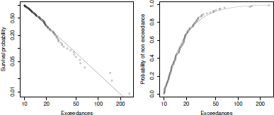
Plotting Pareto tails. The left panel plots the empirical and fitted survival function. The right panel plots the empirical and fitted cumulative distribution function.
It is also possible to plot the cumulative distribution function, given that u is exceeded:
> prob <- rank(danish.exc) / (n.u + 1)
> plot(danish.exc, prob, log = "x", xlab= "Exceedances",
+ ylab = "Probability of non exceedance")
> y = 1 - (x / u)"(-alpha)
> lines(x, y)
6.3.2 Estimation
Although other approaches are possible, in this section we restrict our attention to the maximum likelihood estimator as this approach can easily handle more complex models, for example, the addition of covariates. Maximum likelihood estimation is carried out by optimizing the likelihood of observing a given sample according to the appropriate distribution. For the extreme value distributions discussed here, the optimization must be performed numerically as no analytic solution exists. Further, the case where the shape parameter is zero requires special attention. It is a single point in a continuous parameter space, and as such will not be estimated with probability 1 when optimizing over the generalized extreme value or generalized Pareto likelihoods. The most common approach is to optimize both the generalized extreme value/generalized Pareto likelihoods and the Gumbel/Exponential likelihoods, and apply a significance test (e.g., using the likelihood ratio test, via confidence intervals for the shape parameter) to test whether or not the parameter should be zero.
6.3.2.1 Generalized Extreme Value Distribution
Letting , the i-th block maximum of an observed time series the generalized extreme value log-likelihood for with is given by
Although when the likelihood is not upper bounded anymore because
this is usually not a problem because such small values for ξ correspond to very shorttailed distributions that are unlikely to occur in concrete applications. When , the maximum likelihood estimator is convergent and asymptotically normal when
The following R code computes the negative log-likelihood for the generalized extreme value distribution:
> nllik.gev <- function(par, data){
+ mu <- par[1]
+ sigma <- par[2]
+ xi <- par[3]
+ if ((sigma <= 0) | (xi <= -1))
+ return(1e6)
+ n <- length(data)
+ if (xi == 0)
+ n * log(sigma) + sum((data - mu) / sigma) +
+ sum(exp(-(data - mu) / sigma))
+ else {
+ if (any((1 + xi * (data - mu) / sigma) <= 0))
+ return(1e6)
+ n * log(sigma) + (1 + 1 / xi) *
+ sum(log(1 + xi * (data - mu) / sigma)) +
+ sum((1 + xi * (data - mu) / sigma)^(-1/xi))
+}
+}
Some care is needed when trying to optimize the generalized extreme value likelihood because the likelihood is typically erratic in regions far away from its global maximum and hence numerical optimization might fail. A reasonable strategy is to provide sensible starting values such as the moment estimates for the Gumbel distribution. The following R code does this job for the Danish claim dataset:
> sigma.start <- sqrt(6) * sd(danish.max) / pi
> mu.start <- mean(danish.max) + digamma(l) * sigma.start
> fit.gev <- nlm(nllik.gev, c(mu.start, sigma.start, 0),
+ hessian = TRUE, data = danish.max)
> fit.gev
$minimum
[1] 58.2333
$estimate
[1] 37.7934096 28.9358639 0.6384013
$gradient
[1] -4.878783e-07 2.600457e-07 -7.716494e-06
$hessian
[,1] [,2] [,3]
[1,] 0.03796779 -0.02924794 0.3404126
[2,] -0.02924794 0.03073232 -0.2542531
[3,] 0.34041257 -0.25425309 8.8896897
$code
[1] 1
$iterations
[1] 37
The maximum likelihood estimates can be obtained from fit$estimate and the associated standard errors from
> sqrt(diag(solve(fit.gev$hessian))) #$
[1] 10.7183026 11.0494255 0.4141631
In particular, the maximum likelihood estimates (and the associated standard errors) are
6.3.2.2 Poisson-Generalized Pareto Model
Similar to the generalized extreme value distribution, letting for only those then for the generalized Pareto distribution, the log-likelihood is given by
where m is the number of exceedances above the threshold u, and in the case of ,
As for the generalized extreme value distribution, the log-likelihood can be made arbitrarily large when because
Similar to the generalized extreme value distribution, the maximum likelihood estimator is consistent when and asymptotically normal when
The following R code computes the negative log-likelihood for the generalized Pareto distribution:
> nllik.gp <- function(par, u, data){
+ tau <- par[1]
+ xi <- par[2]
+
+ if ((tau <= 0) | (xi < -1))
+ return(1e6)
+
+ m <- length(data)
+
+ if (xi == 0)
+ m * log(tau) + sum(data - u) / tau
+
+ else {
+ if (any((1 + xi * (data - u) / tau) <= 0))
+ return(1e6)
+
+ m * log(tau) + (1 + 1 / xi) *
+ sum(log(1 + xi * (data - u) / tau))
+ }
+}
The use of the generalized Pareto model for modeling exceedances is a two-step procedure. First, one must optimize the above likelihood and then estimate the rate of exceedances , that is,
For the Danish claim dataset, the likelihood is maximized by invoking
> u <- 10
> tau.start <- mean(danish.exc) - u
> fit.gp <- nlm(nllik.gp, c(tau.start, 0), u = u, hessian = TRUE,
+ data = danish.exc)
> fit.gp
$minimum
[1] 374.893
$estimate
[1] 6.9754659 0.4969865
$gradient
[1] 4.783492e-06 7.958079e-05
$hessian
[,1] [,2]
[1,] 1.138184 5.021902
[2,] 5.021902 75.965994
$code
[1] 1
$iterations
[1] 21
where tau.start is the moment estimator of the exponential distribution. Independently, the rate parameter is easily estimated by with associated standard error . The estimates and related standard errors for the generalized Pareto can be obtained similarly to the generalized extreme value case, and we found = 0.050 (0.004), = 7 (1) and = 0.50 (0.14).
Although from a theoretical point of view the shape parameters of the generalized extreme value and generalized Pareto distributions are the same, the estimates for differ.
It is also possible to use a profile likelihood technique because the main parameter of interest is ξ (see Venzon & Moolgavkar (1988)). Recall that if we consider a parametric model with parameter , define
We can then compute the maximum of the profile log-likelihood
This maximum is not necessarily the same as the (global) maximum obtained by maximizing the likelihood, on a finite sample. Under standard suitable conditions,
so it is possible to derive confidence intervals for . The code will be
> prof.nllik.gp <- function(par,xi, u, data)
+ nllik.gp(c(par,xi), u, data)
> prof.fit.gp <- function(x)
+ -nlm(prof.nllik.gp, tau.start, xi = x, u = u, hessian = TRUE,
+ data = danish.exc)$minimum
> vxi = seq(0,1.8,by=.025)
> prof.lik <- Vectorize(prof.fit.gp)(vxi)
> plot(vxi, prof.lik, type="l", xlab = expression(xi),
+ ylab = "Profile log-likelihood")
> opt <- optimize(f = prof.fit.gp, interval=c(0,3), maximum=TRUE)
> opt
$maximum
[1] 0.496993
$objective
[1] -374.893
> up <- opt$objective
> abline(h = up, lty=2)
> abline(h = up-qchisq(p = 0.95, df = 1), col = "grey")
> I <- which(prof.lik >= up-qchisq(p = 0.95, df = 1))
> lines(vxi[I], rep(up-qchisq(p = 0.95, df = 1), length(I)),
+ lwd = 5, col = "grey")
> abline(v = range(vxi[I]), col = "grey", lty = 2)
> abline(v = opt$maximum, col="grey")
6.3.2.3 Point Process
As alluded to previously, fitting the two-dimensional model better accounts for the uncertainty in estimating these parameters simultaneously. In this case, the log-likelihood to optimize is, using as for the generalized Pareto likelihood (but now with m exceedances from n total observations), given by
and
if and where nb is the number of blocks appearing in the time series.
The following R code computes the negative log-likelihood for the Poisson point process model:
> nllik.pp <- function(par, u, data, n.b){
+ mu <- par[1]
+ sigma <- par[2]
+ xi <- par[3]
+ if ((sigma <= 0) | (xi <= -1))
+ return(1e6)
+ if (xi == 0)
+ poiss.meas <- n.b * exp(-(u - mu) / sigma)
+ else
+ poiss.meas <- n.b * max(0, 1 + xi * (u - mu) / sigma)"(-1/xi)
+ exc <- data[data > u]
+ m <- length(exc)
+ if (xi == 0)
+ poiss.meas + m * log(sigma) + sum((exc - mu) / sigma)
+ else {
+ if (any((1 + xi * (exc - mu) / sigma) <= 0))
+ return(1e6)
+ poiss.meas + m * log(sigma) + (1 + 1 / xi) *
+ sum(log(1 + xi * (exc - mu) / sigma))
+}
+}

As previously, it is desirable to set suitable starting values. For the Poisson point process approach, the starting values are the same as for the generalized extreme value model. The Poisson point process model is fitted by invoking the following code:
> n.b <- 1991 - 1980
> u <- 10
> sigma.start <- sqrt(6) * sd(danish.exc) / pi
> mu.start <- mean(danish.exc) + (log(n.b) + digamma(1)) *
+ sigma.start
> fit.pp <- nlm(nllik.pp, c(mu.start, sigma.start, 0), u = u,
+ hessian = TRUE, data = danishuni[,2], n.b = n.b)
> fit.pp
$minimum
[1] 233.9067
$estimate
[1] 39.8421585 21.8065885 0.4969855
$gradient
[1] 4.518800e-07 -6.474347e-07 1.358003e-05
$hessian
[,1] [,2] [,3]
[1,] 2.524825 -3.631807 76.93413
[2,] -3.631807 5.325742 -114.35596
[3,] 76.934131 -114.355962 2532.88928
$code
[1] 1
$iterations
[1] 43
The maximum likelihood estimates for the Danish claim dataset are Note that the shape parameter estimate is exactly the same as the one we get for the generalized Pareto approach. Further, and the generalized Pareto scale parameter estimate are connected by the relation
6.3.2.4 Other Tail Index Estimates
From Section 6.2.2 (see also Section 6.3.1), if Y has Pareto tails, with tail index , then
or equivalently,
If then should be the opposite of the slope of the linear regression of against (on Figure 6.3, we did plot against , so that the slope was ).
If we consider only the k largest observations (as again, we focus on tails only here), the estimator of is
Hill's estimator (introduced in Hill (1975)) is obtained by assuming that the denominator is almost 1 (which means that k/n is small and n is large):
From asymptotic theory (k should be large, but still, k/n should tend to 0), will be converging to . Further (see Beirlant et al. (2004)),
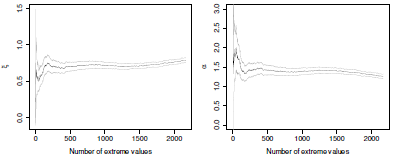
It is possible to obtain (and plot) an asymptotic confidence interval for :
> logXs <- log(sort(danishuni[,2], decreasing=TRUE))
> n <- length(logXs)
> xi <- 1/1:n * cumsum(logXs) - logXs
> ci.up <- xi + qnorm(0.975) * xi / sqrt(1:n)
> ci.low <- xi - qnorm(0.975) * xi / sqrt(1:n)
> matplot(1:n, cbind(ci.low, xi, ci.up),lty = 1, type = "l",
+ col = c("grey", "black", "grey"), ylab = expression(xi),
+ xlab = "Number of extreme values")
Using the delta-method, it is also possible to prove that satisfies
Then it is possible to , and to plot a confidence interval:
> alpha <- 1 / xi
> alpha.std.err <- alpha / sqrt(1:n)
> ci.up <- alpha + qnorm(0.975) * alpha / sqrt(1:n)
> ci.low <- alpha - qnorm(0.975) * alpha / sqrt(1:n)
> matplot(1:n, cbind(ci.low, alpha, ci.up), lty = 1, type = "l",
+ col = c("grey", "black", "grey"), ylab = expression(alpha),
+ xlab = "Number of extreme values")
6.3.3 Checking for the Asymptotic Regime Assumption
There exist some theoretical results about the rate of convergence to the generalized extreme value or Pareto distributions. Unfortunately, they are usually of limited interest because they rely on the knowledge of the distribution of X in which is typically unknown for concrete applications.
If one decides to opt for the block maxima framework, one usually chooses convenient block sizes , for example, n = 365 for daily values and annual maxima, and checks the goodness of fit using standard tools such as quantile-quantile plots. It is more difficult to choose a suitable threshold level as one decides to model threshold exceedances using the generalized Pareto approach or the point process representation. One common way is to check if some specific properties of exceedances above a candidate threshold u are met.
6.3.3.1 Mean Excess Plot
A first strategy relies on the behavior of the expectation of a random variable as u increases. Suppose is generalized Pareto distributed with scale and shape . Then it is not difficult to show that
for all .
Equation (6.13) serves as a basis for choosing a suitable threshold . If for a given is (approximately) generalized Pareto distributed, then the function
is a linear function of u provided that to ensure that is finite.
The conditional expectation is called the mean excess and can be estimated by its empirical version
where is the indicator function and , are i.i.d. random variables. Confidence intervals based on the central limit theorem can also be derived.
The following R function creates the mean excess plot
> meanExcessPlot <- function(data, u.range = range(data),
+ n.u = 100){
+ mean.excess <- ci.up <- ci.low <- rep(NA, n.u)
+ all.u <- seq(u.range[1], u.range[2], length = n.u)
+ for (i in 1:n.u){
+ u <- all.u[i]
+ excess <- data[data > u] - u
+ n.u <- length(excess)
+ mean.excess[i] <- mean(excess)
+ v ar.mean.excess <- var(excess)
+ ci.up[i] <- mean.excess[i] + qnorm(0.975) *
+ sqrt(var.mean.excess / n.u)
+ ci.low[i] <- mean.excess[i] - qnorm(0.975) *
+ sqrt(var.mean.excess / n.u)
+ }
+
+ matplot(all.u, cbind(ci.low, mean.excess, ci.up), col = 1,
+ lty = c(2, 1, 2), type = "l", xlab = "u",
+ ylab = "Mean excess")
+}
If we use this function on the complete dataset, we obtain the graph of Figure 6.6.
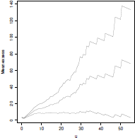
Mean excess plot for the Danish claim data set. The plot seems to be linear above the threshold u =10.
> meanExcessPlot(danish.exc)
Recall that the aim is to detect a suitable threshold u above which the plot appears to be linear—taking into account the estimation uncertainties with the help of the pointwise confidence intervals. For the Danish claim dataset, it seems that there are two possible candidates for u, u = 10 and u = 20. It is more sensible to choose the former because more data will be kept in our analysis.
Remark 6.2 Identifying a suitable threshold using the mean excess plot is usually tricky and highly subjective. Often we will fit extreme value models using several threshold values and check goodness of fit.
6.3.3.2 Parameter Stability
More precisely, let be a generalized Pareto distributed with scale and shape . As stated in Section 6.2.2, because the generalized Pareto distribution is stable by “thresholding” (see Section 6.2.2), a second strategy relies on the behavior of the parameters of a generalized Pareto as the threshold increases. More precisely, if is generalized Pareto distributed with scale and shape , then is generalized Pareto distributed with scale and shape .
The parameter stability procedure consists of plotting
where and are the estimates of the generalized Pareto distribution related to the threshold u, for example, maximum likelihood estimates, and identify regions where the plot remains constant. Usually it is desirable to add confidence intervals on the plot. The parameter stability procedure can be implemented in R with the following code:
> parStabilityPlot <- function(data, u.range = range(data),
+ n.thresh = 50){
+ modified.scales <- rep(NA, n.thresh)
+ shapes <- rep(NA, n.thresh)
+ ci.scales <- ci.shapes <- matrix(NA, 2, n.thresh)
+ all.u <- seq(u.range[1], u.range[2], length = n.thresh)
+ for (i in 1:n.thresh){
+ u <- all.u[i]
+ excess <- data[data > u]
+ tau.start <- mean(excess) - u
+ fit <- nlm(nllik.gp, c(tau.start, 0), u = u, data = excess,
+ hessian = TRUE)
+ mle <- fit$estimate
+ var.cov <- solve(fit$hessian)
+ modified.scales[i] <- mle[1] - mle[2] * u
+ gradient <- c(1, -u)
+ sd.mod.scale <- sqrt(t(gradient) var.cov gradient)
+ ci.scales[,i] <- modified.scales[i] + c(-1, 1) *
+ qnorm(0.975) * sd.mod.scale
+
+ shapes[i] <- mle[2]
+ ci.shapes[,i] <- mle[2] + c(-1, 1) *
+ qnorm(0.975) * sqrt(var.cov[2,2])
+}
+
+ par(mfrow = c(1, 2), mar = c(4, 5, 1, 0.5))
+ plot(all.u, modified.scales, xlab = "u", ylab = "Modified scale",
+ ylim = range(ci.scales))
+ segments(all.u, ci.scales[1,], all.u, ci.scales[2,])
+
+ plot(all.u, shapes, xlab = "u", ylab = expression(xi(u)),
+ ylim = range(ci.shapes))
+ segments(all.u, ci.shapes[1,], all.u, ci.shapes[2,])
+}
Again, if we use this function on the complete dataset, we obtain the graph of Figure 6.7.
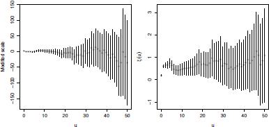
> parStabilityPlot(danishuni[,2], c(0, 50))
6.3.4 Quantile Estimation
For the extreme value distributions, it is easy to obtain quantiles by inverting the distributions. For the GEV distribution, the quantiles are given by
Using the extreme value theory terminology, quantiles are often called return levels—or value at risk for financial applications. For the generalized extreme value distribution, is the return level associated with the return period. Return levels are widely used in concrete applications because they have a convenient interpretation.
To see this, let be independent copies of a random variable and a quantile of X such that . Consider the first occurrence where the exceed the level , that is,
Clearly, the random variable I follows a geometric distribution where the probability to have success at each trial is . This implies that , or in other words, that the quantile is expected to be exceeded once every trials. For the generalized extreme value distribution, assuming that the are annual maxima, the return level would be expected to be exceeded once every years.
It is important to mention that the notion of return period does not imply any periodicity in the occurrence of extreme events because within each block (typically years), there is the same chance of exceeding the level . Furthermore, the notion of a return period does not make sense in the case of non-stationarity; for example, the random variables are still independent but do not share the same distribution.
For the generalized Pareto distribution, one must account for the frequency of occurrence of exceedances in order to define return levels because this distribution is usually used for modeling values given that we exceed a threshold u. We then have to solve
where
It is not difficult to show that the return levels are
where .
Using similar arguments as those used for the generalized extreme value distribution, the return level is expected to be exceeded once every observations. For practical reasons, it is often more convenient to modify to a suitable scale. For example if we observed daily values, then the return levels xp would be expected to be exceeded once every years with .
It is common in extreme value analysis to plot the return levels as the return period increases. Such a plot is called a return level plot and consists of plotting the function
for the generalized extreme value distribution and
for the generalized Pareto distribution.
Figure 6.8 shows return levels plots for both the generalized extreme value and the generalized Pareto distributions with different values for the shape parameter . Typically, return level plots use a logarithmic scale for the x-axis so that the Gumbel/Exponential cases, that is, = 0, appear as a straight line—at least for large return periods. As expected, the cases yield the largest return levels because, in such a situation, the distribution is not upper bounded.
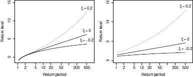
Return level plots for different values of the shape parameterξ . The left panel corresponds to the generalized extreme value distributions with The right panel corresponds to the generalized Pareto distribution with .
To estimate quantiles, plug in the maximum likelihood estimates in (6.14) or (6.15) depending on the model considered. For the point process characterization (6.12), quantile estimates are given by that of the generalized Pareto distribution with scale and shape .
6.4 Model Checking
Although our statistical models are based on asymptotic theory, that is, (6.3) and (6.8), it is wise (as for any statistical model) to check whether our modeling is accurate. There is nothing specific to extreme values here, and standard graphical checks such as quantile- quantile or probability-probability plots are widely used. We will see how return levels can be used to assess goodness of fit. Whatever graphical tool is used, they all rely on the same idea: comparing what we get (the data) to what would expect from the model (the fitted values).
6.4.1 Quantile Quantile Plot
A first strategy is to compare quantiles. The idea is the following. For each ordered observation , we associate the corresponding empirical non-exceedance probability
that is, we treat the ordered observation as a sample quantile with non exceedance probability . The model counterpart of each is the estimated quantiles associated with the non-exceedance probabilities ,i.e., in (6.14) or in (6.15). Note that for the generalized Pareto case, we have to set in (6.15) because the quantile-quantile plot focus is only on exceedances and not all of the data.
The quantile quantile plots for the generalized extreme value and generalized Pareto distributions plot, respectively, the points
If the model is correct, then these points should lie approximately around the y = x line.
The following R code produces a quantile-quantile plot for the generalized Pareto distribution:
> qqgpd <- function(data, u, tau, xi){
+ excess <- data[data > u]
+ m <- length(excess)
+ prob <- 1:m / (m + 1)
+ x.hat <- u + tau / xi * ((1 - prob)^-xi - 1)
+
+ ylim <- xlim <- range(x.hat, excess)
+ plot(sort(excess), x.hat, xlab = "Sample quantiles",
+ ylab = "Fitted quantiles", xlim = xlim, ylim = ylim)
+ abline(0, 1, col = "grey")
+}
> qqgpd(danishuni[,2], 10, 7, 0.5)
The left panel of Figure 6.9 shows the quantile-quantile plot obtained from the fitted generalized Pareto distribution. We can see that most of the points lie around the y = x line, indicating a good fit. Although the three largest deviate from the y = x line, it is not worrying because these points are associated to the largest plotting position uncertainties.
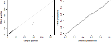
Model checking for the fitted generalized Pareto distribution to the Danish claim dataset.
6.4.2 Probability—Probability Plot
The idea behind the probability-probability plot is almost the same but compares non- exceedance probabilities instead of quantiles. Given the empirical non-exceedance probabilities (6.18), we compute for each observation the estimated non-exceedance probability from the fitted model. For the generalized extreme value distribution, we have
while for the generalized Pareto distribution, it is given by
The probability-probability plots for the generalized extreme value and generalized Pareto distribution plot, respectively, the points
and, similar to the quantile-quantile plot, points lying around the y = x line indicate a good fit.
The following R code produces a probability-probability plot for the generalized Pareto distribution:
> ppgpd <- function(data, u, tau, xi){
+ excess <- data[data > u]
+ m <- length(excess)
+ emp.prob <- 1:m / (m + 1)
+ prob.hat <- 1 - (1 + xi * (sort(excess) - u) / tau)"(-1/xi)
+ plot(emp.prob, prob.hat, xlab = "Empirical probabilities",
+ ylab = "Fitted probabilities", xlim = c(0, 1),
+ ylim = c(0, 1))
+ abline(0, 1, col = "grey") +}
> ppgpd(danishuni[,2], 10, 7, 0.5)
The left panel of Figure 6.9 shows the probability-probability plot for the fitted generalized Pareto distribution. Similar to the quantile-quantile plot, most of the points lie around the y = x line, indicating a good fit.
6.4.3 Return Level Plot
In Section 6.3.4 we introduced the notion of return levels and return periods. These two concepts can be used to check the goodness of fit of our model. Note that return level plots are not only restricted to model checking.
The use of return level plots for model checking is to plot the fitted return level curve as in Figure 6.8 and compare it to the data. In other words, it is a kind of mix between the two previous tools because the x-axis plots (some kind) of probability, as in the probability- probability plot while the y-axis plots quantiles as in the quantile-quantile plot.
First, based on our fitted model, we produce a return level plot using (6.14) or (6.15). The second step involves adding the observations to this plot. As in Section 6.4.1, for each ordered observation , we associate the corresponding empirical return period based on (6.18). For the generalized extreme value distribution, and because , the empirical return periods are
and the following points are added to the return level plot,
For the generalized Pareto model, it is a little bit more complicated because the return period depends on the probability of observing an exceedance and the number of observation per block, for example, year, . Because, in that case, , the empirical return periods are
and the following points are added to the return level plot,
Remark 6.3 There is no contradiction in saying that in such cases, instead of as in Section 6.3.4. While the former uses the conditional non-exceedance probability , the latter is unconditional, that is,
The following R code produces return level plots for the generalized Pareto model:
> rlgpd <- function(data, u, tau, xi, nb){
+ excess <- data[data > u]
+ n <- length(data)
+ m <- length(excess)
+ zeta.u <- m / n +
+ rl <- function(T){
+ prob <- 1 - 1 / (nb * T)
+ u + tau / xi * (((1 - prob) / zeta.u)"-xi - 1)
+}
+
+ plot(rl, from = 1 / nb + 0.1, to = 100, log = "x",
+ xlab = "Return period", ylab = "Return level")
+
+ points((m+1) / (nb * zeta.u * m:1), sort(excess))
+}
Because the Danish dataset has irregularly spaced observations, it is necessary to appropriately set nb. We use nb = 365 x 2,167/4,015 = 197 as there are 2,167 claims, 4,015 consecutive days of observations, and we want return levels on an annual scale. The corresponding return level plot is obtained by invoking
> rlgpd(danishuni[,2], 10, 7, 0.5, 197)
Figure 6.10 plots two return level plots for the Danish claim dataset based on ex- ceedances. Apart from the three largest observations, all the points lie around the fitted return level curve. For pedagogical reasons, we artificially set the largest claim to 500 million Danish Kroner in the right panel. As expected, the largest claim lies far away from the fitted return level curve. But because it is based on ranks, the associated empirical return period remains the same. Although extreme value theory aims at modeling the most severe events, this example is illuminating because it says that one should not focus too much on the largest observations in a return level plot because these observations are associated with the largest uncertainties. Further, it is heavily recommended to add confidence intervals to return level plots either using bootstrap or the delta method on the fitted quantiles.
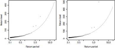
Checking the goodness of fit of the generalized Pareto distribution to the Danish claim dataset using return level plots. The left panel plots the points defined by (6.18) while the right panel still uses (6.18) but the largest claim has been artificially set to 500 millions Danish Kroner.
6.5 Reinsurance Pricing
Consider observations, over k years. In year i, losses were observed. For convenience, let denote reported losses, for year (of occurrence) i. One can imagine some inflation index , so that we have to replace original observations with adjusted (or normalized) losses 's. For instance, in Pielke et al. (2008), to adjust losses related to tropical cyclones (U.S. mainland damage), consider the function of the GNP inflation index, a wealth factor index, and an index to take into account coastal county population change. This index can be visualized on Figure 6.11, with actual economic losses, on the left, and normalized losses, on the right.
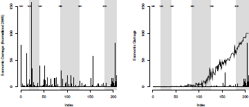
Economic losses on U.S. mainland, due to tropical cyclones, actual versus normalized losses.
> plot(base$Base.Economic.Damage/1e9,type="h",
+ ylab="Economic Damage",ylim=c(0,155))
> lines(base$Base.Economic.Damage/base$Normalized.PL05*100,lwd=2)
> plot(base$Normalized.PL05/1e9,type="h",
+ ylab="Economic Damage (Normalized 2005)",ylim=c(0,155))
For damages due to tropic cyclones, we consider an adjustment factor function of inflation, wealth, and population increase. For aviation losses, it is common to take into account fleet value, and passenger per kilometers flown.
Consider here a standard nonproportional reinsurance contract, namely an excess of loss treaty C xs D with deductible D and an upper limit C, in excess of the deductible. The upper limit is then C + D. For the reinsurance company, the cost of a claim with economic loss X will be , while for the (direct) insurance company, the cost is . For convenience, let denote the loss function, from the reinsurer's point of view,
Some specific contracts can be found to deal with aggregate losses, the so-called stop-loss treaties. For year i, one can consider either
where reinsurance is used for all contracts, or
where an excess of loss treaty is considered, on the overall loss, with aggregate deductible AD and aggregate cover AC. A reinsurance treaty is said to have k reinstatements if AC = (k +1).C.
6.5.1 Modeling Occurence and Frequency
In this section and the next, we will use an approach similar to the one used in Schmock (1999). Consider the number of tropical storms per year. Using table() , we will get counts only for years that appear in the dataset (which experienced a tropical cyclone). So we need to add a 0 to the years that did not appear in the names of the table object:
> TB <- table(base$Year)
> years <- as.numeric(names(TB))
> counts <- as.numeric(TB)
> years0=(1900:2005)[which(!(1900:2005)%in%years)]
> db <- data.frame(years=c(years,years0),
+ counts=c(counts,rep(0,length(years0))))
> db[88:93,]
years counts
88 2003 3
89 2004 6
90 2005 6
91 1902 0
92 1905 0
93 1907 0
A natural idea can be to assume that , with a constant intensitys ,
> mean(db$counts)
[1] 1.95283
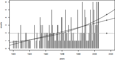
One can also consider that the intensity cannot be considered constant with time if we look at Figure 6.12. Two models will be considered here. A first one will be obtained when is assumed to be affine in i:
> reg0 <- glm(counts~years,data=db,family=poisson(link="identity"),
+ start=lm(counts~years,data=db)$coefficients)
(Observe that we have to specify starting values for the algorithm to ensure that the numerical algorithms converge; see Chapter 14 for a discussion). An alternative can be to consider a standard Poisson regression, with a logarithm link function, so that will be exponentially growing (or decaying) with i:
> regl <- glm(counts~years,data=db,family=poisson(link="log"))
Those three models can be compared on Figure 6.12:
> plot(years,counts,type='h',ylim=c(0,6),xlim=c(1900,2020))
> cpred1=predict(reg1,newdata=data.frame(years=1890:2030),type="response")
> lines(1890:2030,cpred1,lwd=2)
> cpred0=predict(reg0,newdata=data.frame(years=1890:2030),type="response")
> lines(1890:2030,cpred0,lty=2)
> abline(h=mean(db$counts),col="grey")
If we want to price a reinsurance contract for 2015, we need a prediction of that specific year:
> cbind(constant=mean(db$counts),linear=cpred0[126],exponential=cpred1[126])
constant linear exponential
126 1.95283 3.573999 4.379822
Observe that other datasets can be used to model the number of landfalling tropical storms, such as MacAdie et al. (2009).
6.5.2 Modeling Individual Losses
Two adjustments were considered in Pielke et al. (2008):
> hill(base$Normalized.PL05)
> hill(base$Normalized.CL05)
Assume that a company has a 5% market share, so that we can assume that if a loss is X, the insurance company will pay X/20.

Consider a threshold of c0 = 0.5, so that above that threshold, we assume that losses have a GP distribution. Note that 12.5% of the storms exceed that threshold (the same percentage using Normalized.CL05 and Normalized.PL05):
> threshold=.5
> mean(base$Normalized.CL05/1e9/20>.5)
[1] 0.1256039
Above co, parameters of the GP distribution are
> (gpd.CL <- gpd(base$Normalized.CL05/1e9/20,threshold)$par.ests)
xi beta
0.3634010 0.7122717
> (gpd.PL <- gpd(base$Normalized.PL05/1e9/20,threshold)$par.ests)
xi beta
0.4424669 0.6705315
Then we should compute
where G denotes the Pareto distribution.
> E <- function(yinf,ysup,xi,beta){
+ as.numeric(integrate(function(x) (x-yinf)*dgpd(x,xi,mu=threshold,beta),
+ lowe=yinf,upper=ysup)$value+
+ (1-pgpd(ysup,xi,mu=threshold,beta))*(ysup-yinf))
+}
> E(2,6,gpd.PL[1],gpd.PL[2])
[1] 0.3309865
> E(2,6,gpd.CL[1],gpd.CL[2])
[1] 0.3058124
The pure premium is then
where the first term is the expected number of landfall storms, the second term is the probability that the loss exceeds the threshold, and the third term is the expected reinbursment of a reinsurance treaty, given that threshold c0 has been exceeded. Here, if we consider a linear model for frequency, the pure premium of a nonproportional contract, with deductible 2 and cover 4, will be
> cpred1[126]*mean(base$Normalized.CL05/1e9/20>.5)*
+ E(2,6,gpd.CL[1],gpd.CL[2])
126
0.05789891
(in USD billions). A company with 5% market share should be ready to pay a 5.789 million USD premium to have a reinsurance cover, in excess of 2 billion, with a limited cover of 4 billion.