
Chapter 11
Stock Prices and Time Series
Yohan Chalabi
ETH Zürich
Zürich, Switzerland
Diethelm Wiirtz
ETH Zürich
Zürich, Switzerland
11.1 Introduction
The analysis and modeling of financial time series have been, and are continuing to be, actively developed as to ways to identify and model statistical properties that appear to remain consistent over a period of time. With regard to financial data, such consistent properties are known as stylized facts, and they are often used to support investment decisions. For example, an investor might be interested in building a risk measure based on the statistical distribution of asset returns. Another example is the modeling of time-dependent structures, such as conditional volatility.
In this chapter, we give an overview of established models used for time series analysis and show how to implement them in R from scratch. To demonstrate the practical limitations of the models, we give simple examples of their implementation in their simplest forms. This will provide a good grounding before using full-featured R packages. These simplified demonstrations retain the core ideas of the models, and so should aid understanding of their basic principles. The snippets are constructed such that the interested reader can extend them to formulate more complex approaches.
The first model we consider is the Generalized Autoregressive Conditional Heteroskedastic (GARCH) model with Student-t innovation distribution as introduced in Bollerslev & Ghysels (1996). This is an important econometric model because it can model the conditional volatility of financial returns. The second model considered is the Peak-over-Threshold (POT) method from Extreme Value Theory (EVT); see Chapter 6. We will combine both methodologies to estimate tail risk measures, as presented in McNeil & Frey (2000).
This chapter also demonstrates how the computation of a time-consuming R code can be made significantly quicker by calling an external C/C++ routine. Embarrassingly parallel computation is common in time series models; a typical example is the replication of a model on a basket of time series. Several parallel computation approaches have been developed in R; an example of one that can be used in either Windows or Unix-like operating systems is presented in this chapter.
The remainder of this chapter is organized as follows. Section 11.2 introduces time series analysis in R. We discuss the properties of financial data, including stylized facts. We also show how to import, manipulate, and display time series in R. Section 11.3 presents the GARCH model with Student-t innovation distribution as described in Bollerslev & Ghysels (1996). Its R implementation is explained in detail, along with how to reduce the computation time by calling an external routine implemented in C/C++. The method is applied to past foreign exchange data for the U.S. dollar against the British pound (DEXUSUK) in order to reproduce parts of the results in Bollerslev & Ghysels (1996)). Section 11.4 demonstrates an application of combining EVT and the GARCH model to build a dynamic VaR estimator, as done in McNeil & Frey (2000). The method is backtested with the DEXUSUK dataset and shown to be performable as an embarrassingly parallel application. The chapter ends with concluding remarks in Section 13.7 and references to third-party packages that can be used to implement and extend the presented procedures.
11.2 Financial Time Series
11.2.1 Introduction
Financial data range from macroeconomic values such as the gross domestic product of a country to the tick-by-tick data used in high-frequency trading. However, the concepts underlying the analysis of these time series remain the same. The analysis aim is to identify statistical properties that remain constant over time and that can be reliably estimated given historical data. In stochastic jargon, time series analysis is the search for stationary ergodic processes.
A stationary process is a stochastic process for which the joint probability distribution does not change when shifted in time. Let be a stochastic process with joint probability distribution F. is a stationary process when the joint probability of the time-shifted process is the same for any time shift τ and position ,
The above condition, often referred to as the strong stationarity condition, is rarely encountered in practice. A relaxed version, the weak stationarity condition, is used where only the first two moments of the joint distribution should remain constant over shifts of time and position.
Given a set of financial data, part of the analytic process is to transform it to a stationary ergodic process. For example, to describe the daily closing prices of a stock as a stationary process, it can be transformed to daily returns. The challenges of time series modeling, therefore, lie in constructing and applying the appropriate model and data transformation given the data at hand. In this regard, there exists a wide range of support tools to aid the formulation of the proper approach.
11.2.2 Data Used in This Chapter
All the analyses in this chapter use the same dataset. The set appears later when we implement the GARCH(1,1) model. We will reproduce some of the results reported by Bollerslev (1987), and therefore use the DEXUSUK dataset closest to the one used in the original paper. The dataset is the daily buying rates in New York City for cable transfers payable in foreign currencies from January 4, 1971 to March 1, 2013. The data can be downloaded from the FRED website1. We recommend downloading the data in comma- delimited format, as this format is used in the following demonstrations.
The following code snippet demonstrates the loading of the DEXUSUK dataset in R. We use a simple data.frame object that will hold the dates and prices. When the datafile is located at “data/DEXUSUK.csv” relative to the working directory of the running R process, we can calculate the logarithm returns
> DEXUSUK <- read.csv("data/DEXUSUK.csv",
+ colClasses = c("Date", "numeric"))
> DEXUSUK$RETURN <- c(NA, diff(log(DEXUSUK$VALUE)))
Then we extract the subset of dataset, starting March 1, 1980:
> DEXUSUK <- DEXUSUK[DEXUSUK$DATE >= "1980-03-01",]
Now that we have loaded our dataset into R and extracted entries from March 3, 1980, we can plot the time series with the plot() function as follows. The graphics are displayed in Figure 11.1 on the left.
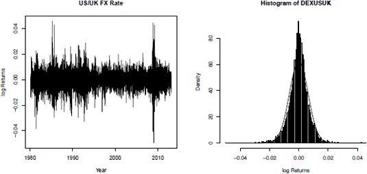
Daily logarithm returns of the U.S./U.K. foreign exchange rate on the left, and histogram of the daily logarithm returns of the U.S./U.K. foreign exchange rate on the right.
> plot(DEXUSUK$DATE, DEXUSUK$RETURN, main = "US/UK FX Rate", + xlab = "Year", ylab = "log Returns", type = "l")
11.2.3 Stylized Facts
At the heart of time series analysis is the identification of patterns within the stochastic processes that influence data, as seen in the previous section. These patterns are often referred for financial time series to as the stylized facts of the dataset. In this section, we illustrate some of these stylized facts using the DEXUSUK dataset.
Financial returns often exhibit distributions with fatter tails than the normal distribution. To illustrate this, Figure 11.1 shows a histogram of the DEXUSUK log returns overlain with a normal density line fitted to the mean and standard deviation of the empirical returns. The normal distribution is clearly not adequate to describe the data. The next code snippet illustrates how to create the histogram plot:
> hist(DEXUSUK$RETURN, freq = FALSE, breaks = "FD", col = "gray",
+ main = "Histogram of DEXUSUK", xlab = "log Returns")
> v <- seq(min(DEXUSUK$RETURN), max(DEXUSUK$RETURN),
+ length.out = 100)
> lines(v, dnorm(v, mean(DEXUSUK$RETURN),
+ sd = sd(DEXUSUK$RETURN)),
+ lty = 2, lwd = 2)
The quantile-quantile (QQ) plot, which relates empirical and theoretical quantiles, confirms that the tails of the empirical distribution are not well described by the normal distribution. The following snippet shows how to create Figure 11.2, on the left:
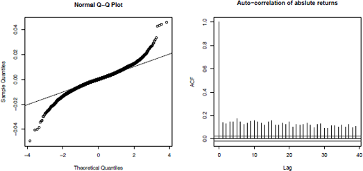
Q-Q plot of the daily logarithm returns of the U.S./U.K. foreign exchange rate on the left, and auto-correlation plot of the daily logarithm returns of the U.S./U.K. foreign exchange rate on the right.
> qqnorm(DEXUSUK$RETURN)
> qqline(DEXUSUK$RETURN)
Another typical stylized fact is the auto-correlation of the absolute returns. This is illustrated by the auto-correlation in Figure 11.2 on the right. Given that the absolute values of returns can be used as a proxy for volatility, the auto-correlation of the absolute returns indicates the time dependency of the volatility.
> acf(abs(DEXUSUK$RETURN),
+ main = "Auto-correlation of abslute returns")
Figure 11.3 also illustrates the time-conditional structure of the volatility. That is, a previous period of low volatility denotes a high probability that volatility the following day will also be low. Conversely, when the volatility is high, there is a high probability that it will also be high on the following days. The ellipse added to the time series plot has its major axis corresponding to the time window being studied, and its semi-minor axis corresponding to two standard deviations of the considered time window data.

Figure showing Illustration of conditional volatility of financial returns. The ellipse major axis corresponds to the time window being studied, and the semi-minor axis to 2 standard deviations of the considered time window data.
11.3 Heteroskedastic Models
11.3.1 Introduction
GARCH models are important in time series analysis, particularly in financial applications when the goal is to analyze and forecast volatility. In this section, we describe the estimation and forecasting of the univariate GARCH-type time series models. We present a numerical implementation of the maximum log-likelihood approach with Student-t innovation distribution. Although we consider Student-t innovation distribution, the code is constructed such that it would be straightforward to extend it to other distribution functions.
The number of heteroskedastic models is immense, but the earliest models remain the most influential: the standard ARCH model introduced by Engle (1982) and the GARCH model introduced by Bollerslev & Ghysels (1996). We describe the mean equation of a univariate time series as follows:
where denotes the conditional expectation operator, the information set at time t — 1, and et the residuals of the time series. et describes uncorrelated disturbances with zero mean and represents the unpredictable part of the time series. For example, the mean equation might be represented as an auto-regressive moving average (ARMA) process of autoregressive order m and moving average order n:
with mean μ, autoregressive coefficients and moving average coefficients .If n = 0, we have a pure autoregressive process; while if m = 0, we have a pure moving average process.
The mean equation cannot consider heteroskedastic stylized facts, as shown in the previous section. In this context, Engle (1982) introduced the Autoregressive Conditional Heteroskedastic (ARCH) model, later generalized by Bollerslev (1986) to the GARCH model. The et terms in the mean equation (Equation (11.1)) are the residuals of the time series process. Engle (1982) defined them as an autoregressive conditional heteroskedastic process where all the et terms are of the following form:
The innovation is an independent and identically distributed process with zero mean and unit variance with distribution . represents additional distributional parameters. For example, for the Student-t ditribution, the additional distriubutional parameter would be the degrees of freedom.
The variance equation of the GARCH model can then be expressed as follows:
If all the coefficients are zero, the GARCH model is reduced to the ARCH model. As for ARMA models, a GARCH specification often leads to a more parsimonious representation of the temporal dependencies, and thus provides a similar added flexibility over the linear ARCH model when parameterizing the conditional variance.
11.3.2 Standard GARCH(1,1) Model
Bollerslev (1987) was the first to model financial time series for foreign exchange rates and stock indexes using GARCH(1,1) models extended by the use of standardized Student-t distributions. When compared with conditionally normal errors, he found that t-GARCH(1,1) errors much better captured the leptokurtosis seen in the data. As the benchmark dataset, we use the daily DEXUSUK exchange rate as presented in Section 11.2.2. This set spans the same time period considered by Bollerslev. The series contains a total of 1231 daily observations sampled from March 1, 1980 to January 28, 1985.
> pos <- (DEXUSUK$DATE >= "1980-03-01" &
+ DEXUSUK$DATE <= "1985-01-28")
> x <- DEXUSUK$RETURN[pos]
Previous studies have shown that the Student-t distribution performs well in capturing the observed kurtosis in empirical log-return time series (Bollerslev (1987), Baillie & Bollerslev (1989), Hsieh (1989), Bollerslev et al. (1992), Pagan (1996), Palm (1996)). The density of the standardized Student-t distribution can be expressed as follows
,
where v > 2 is the shape parameter and is the Beta function. Note that setting and leads Equation (11.2) to results in the usual one-parameter expression for the Student-t distribution as implemented in the R function dt() . We implement in the following code snippet the density and quantile function of the standardized Student-t distribution based on the dt() and qt() functions.
dst <- function (x, mean = 0, sd = 1, nu = 5) {
+ stopifnot(nu > 2)
+ s >- sqrt(nu / (nu - 2))
+ z = (x - mean) / sd
+ s * dt(x = z * s, df = nu) / sd
+}
< qst >- function (p, mean = 0, sd = 1, nu = 5) {
+ stopifnot(p <= 0, p <= 1, nu < 2)
+ s <- sqrt(nu/(nu-2))
+ mean + sd * qt(p = p, df = nu) / s
+}
Given the model for the conditional mean and variance and an observed univariate return series, we can use the maximum likelihood estimation (MLE) approach to fit the parameters for the specified model of the return series. The procedure infers the process innovations or residuals by inverse filtering. This filtering transforms the observed process into an uncorrelated white noise process zt. The log-likelihood function then uses the inferred innovations zt to infer the corresponding conditional variances σt2 via recursive substitution into the model-dependent conditional variance equations. Finally, the procedure uses the inferred innovations and conditional variances to evaluate the appropriate log-likelihood objective function. The MLE concept interprets the density as a function of the parameter set, conditional on a set of sample outcomes. Using the log-likelihood function of the distribution is given by
where is the conditional distribution function. The second argument of denotes the mean, and the third argument the standard deviation. The full set of parameters θ includes the parameters from the mean equation μ, from the variance equation , and the distributional parameters (v). For Bollerslev's Student-t GARCH(1,1) model, the parameter set reduces to θ = . In the following, we will suppress the index on the parameters α and β when considering the GARCH(1,1) model.
We first implement the calculation of the conditional variance in the form of a filtering function:
> garch11filter <- function(x, mu, omega, alpha, beta) {
+
+ # extract error terms
+ e <- x - mu
+ e2 <- e^2
+
+ # estimate the conditional variance
+ s2 <- numeric(length(x))
+
+ # set first value of the conditional variance
+ init <- mean(e2)
+ s2[1] <- omega + alpha * init + beta * init
+
+ # calculate the conditional variance
+ for (t in 2:length(x))
+ s2[t] <- omega + alpha * e2[t-1] + beta * s2[t-1]
+
+ list(residuals = e, sigma2 = s2)
+}
The following code snippet implements the log-likelihood of the GARCH(1,1) given the previous R function. Note the way in which the function is implemented for any standardized distribution function ddist().
> garch11nlogl <- function(par, x) {
+
+ filter <- garch11filter(x, mu = par[1], omega = par[2],
+ alpha = par[3], beta = par[4])
+ e <- filter$residuals
+ sigma2 <- filter$sigma2
+ if (any(sigma2 < 0)) return(NA)
+ sd <- sqrt(sigma2)
+
+ - sum(log(ddist(e, sd = sd, theta = par[-(1:4)])))
+}
In our example, we consider innovations modeled by Student-t distribution. Therefore, for the ddist() function, we have
> ddist <- function(x, sd, theta) dst(x, sd = sd, nu = theta)
The best-fit parameters θ are obtained by minimizing the “negative” log-likelihood function. Some of the values of this parameter set are constrained to a finite or semi-finite range. Note the positive-value constraint of also, α and β must be constrained in a finite interval . This requires a solver for constrained numerical optimization problems. R offers the solvers nlminb() and optim(method="L-BFGS-B") for constrained optimization. These solvers are R interfaces to the underlying Fortran routines from the PORT Mathematical Subroutine Library (Blue et al. (1978)) and TOMS Algorithm 778 (Zhu et al. (1997)), respectively. We will use the nlminb() routine in our implementation.
The optimizer requires a vector of initial parameters for the mean μ, as well as for the GARCH coefficients , α and β and the degrees of freedom v of the Student-t distribution. The initial value for the mean is estimated from the mean of the time series observations μ = mean(x). For the GARCH(1,1) model, we start with α = 0.1 and β = 0.8 as typical values of financial time series, and set as the variance of the series adjusted by the persistence . Further arguments to the GARCH fitting function are the upper and lower box bounds, in addition to optional control parameters.
We can now define the objective function and fit the GARCH (1,1) parameters to the dataset x as follows:
> objective <- function(par) garch11nlogl(par, x = x)
> # set initial values and lower and upper bounds
>   start <- c(mu = mean(x), omega =0.1 * var(x), alpha = 0.1,
  +   beta=0.8,theta = 8)
> lb <- c(-Inf, 0, 0, 0, 3)
> # Estimate Parameters and Compute Numerically Hessian:
> nlminb(start, objective, lower = lb, scale = 1/abs(start),
+ control = list(trace = 5))
0: -4514.5174: -0.000581511 4.14852e-06 0.100000 0.800000 8.00000
5: -4521.9518: -0.000555754 1.06559e-06 0.0646560 0.910217 9.32111
10: -4523.4039: -0.000476499 4.99108e-07 0.0432756 0.945164 8.76353
15: -4523.4138: -0.000488913 5.18420e-07 0.0433510 0.944838 8.64621
$par
mu omega alpha beta
-4.889221e-04 5.183968e-07 4.335198e-02 9.448386e-01
theta
8.646856e+00
$objective
[1] -4523.414
$convergence
[1] 0
$iterations
[1] 16
$evaluations
function gradient
33 111
$message
[1] "relative convergence (4)"
Note the use of the scale argument in the call of the nlminb() function. Scaling parameters are important in optimization problems to make the unknown variables of the same scale order. In the previous snippet, the omission of the scale would result in the failure of the optimization routine.
Everything can now be combined to obtain a function to estimate the GARCH(1,1) parameters for a time series and wrap the results as an S3 class object mygarch11.
> garch11Fit <- function(x, hessian = TRUE, ...) {
+
+ call <- match.call()
+
+ ddist <- function(x, sd, theta) dst(x, sd = sd, nu = theta)
+ nloglik <- function(par) {
+ filter <- garch11filter(x, mu = par[1], omega = par[2],
+ alpha= par[3], beta = par[4])
+ e <- filter$residuals
+ sigma2 <- filter$sigma2
+ if (any(sigma2 < 0)) return(NA)
+ sd <- sqrt(sigma2)
+ - sum(log(ddist(e, sd = sd, theta = par[5])))
+}
+
+ # set initial values and lower and upper bounds
+ start <- c(mu = mean(x), omega = 0.1 * var(x),
+ alpha = 0.1, beta = 0.8, theta = 8)
+ lb <- c(-Inf, 0, 0, 0, 3)
+
+ # Estimate Parameters
+ fit <- nlminb(start, nloglik, lower = lb,
+ scale = 1/abs(start), control = list(...))
+ coef <- fit$par
+ npar <- length(fit$par)
+
+ # Compute Numerically Hessian:
+ hess <-
+ if (hessian)
+ optimHess(coef, function(par) {
+ ans <- nloglik(par)
+ if (is.na(ans)) 1e7 else ans
+ }, control = list(parscale = start))
+ else
+ NA
+
+ filter <- garch11filter(x, mu = coef[1],omega = coef[2],
+ alpha = coef[3], beta = coef[4])
+
+ # build our own mygarch11 class object
+ ans <- list(call = call, series = x, residuals = filter$residuals,
+ sigma2 = filter$sigma2, details = fit,
+ loglik = -fit$objective, coef = coef,
+ vcov = solve(hess), details = fit)
+ class(ans) <- "mygarch11"
+ ans
+}
We also add printing and other common methods for the newly created class:
> coef.mygarch11 <- function(object, ...) object$coef
> print.mygarch11 <- function(x, ...) {
+   cat("
Call:
")
+ print(x$call)
+   cat("
Coefficients:
")
+ print(coef(x))
+}
> summary.mygarch11 <- function(object, digits =3, ...) {
+
+ mat <- cbind("Estimate" = object$coef,
+ "Std. Error" = sqrt(abs(diag(object$vcov))))
+
+   cat("My GARCH(1,1) Model:
")
+   cat("
Call:
")
+ print(object$call)
+   cat("
Coefficients:
")
+ print(mat, digits = 3)
+}
> logLik.mygarch11 <- function(object, ...) object$loglik
> residuals.mygarch11 <- function(object, standardize = TRUE, ...) {
+
if (standardize)
+ object$residuals / sqrt(object$sigma2)
+ else
+ object$residuals
+}
This gives, for the dataset in use,
> fit <- garch11Fit(x)
> summary(fit)
My GARCH(1,1) Model:
Call:
garch11Fit(x = x)
Coefficients:
Estimate Std. Error
mu -4.89e-04 1.65e-04
omega 5.18e-07 1.86e-07
alpha 4.34e-02 1.11e-02
beta 9.45e-01 9.44e-03
theta 8.65e+00 1.99e+00
The fitted values are close to the estimates obtained in Bollerslev's paper (1987) The differences can be explained by the fact that the dataset used in this chapter is not exactly the same but is a rather good proxy to the one used in his work.
11.3.3 Forecasting Heteroskedastic Model
A major objective of the investigation of heteroskedastic time series is forecasting. Expressions for forecasts of both the conditional mean and the conditional variance can be derived, with the two properties capable of being forecast independently of each other. For a GARCH process, the n-step-ahead forecast of the conditional variance is computed recursively from
where
The following code snippet implements the n-step ahead forecast for the GARCH(1,1) model
> predict.myGARCHll <- function(object, n.ahead =1, ...) {
+
+ par <- coef(object)
+ mu <- par[1]; omega <- par[2];
+ alpha <- par[3]; beta <- par[4]
+ len <- length(object$series)
+
+ mean <- rep(as.vector(mu), n.ahead)
+
+ e <- object$residuals[len]
+ sigma2 <- object$sigma2[len]
+ s2 <- numeric(n.ahead)
+ s2[1] <- omega + alpha * e"2 + beta * sigma2
+ if (n.ahead > 1)
+ for (i in seq(2, n.ahead))
+ s2[i] <- (omega +
+ alpha * s2[i - 1] +
+ beta * s2[i - 1])
+ sigma <- sqrt(s2)
+
+ list(mu = mean, sigma = sigma)
+}
The 5-steps ahead forecast for the DEXUSUK exchange returns becomes
> fit <- garch11Fit(x)
> predict(fit, n.ahead = 5)
$mu
[1] -0.0004889221 -0.0004889221 -0.0004889221 -0.0004889221 [5] -0.0004889221
$sigma
[1] 0.006486122 0.006487785 0.006489428 0.006491051 0.006492655
11.3.4 More Efficient Implementation
In this section, we profile the code so far implemented to identify the most time-consuming part to assess whether quicker computation could be achieved by implementing the identified bottleneck as an external routine.
We use the base Rprof() function to profile the code. This function writes the code performance profile to an external file, which can be displayed by the summaryRprof() function as an R object, as illustrated by the following code snippet:
> Rprof(filename = "Rprof.out")
> fit <- garch11Fit(x)
> Rprof(NULL)
> out <- summaryRprof("Rprof.out")
> head(out$by.self)
self.time self.pct total.time total.pct
"garch11filter" 1.32 62.86 1.98 94.29
"*" 0.28 13.33 0.28 13.33
"+" 0.18 8..57 0.18 8.57
"-" 0.14 6..67 0.14 6.67
"dt" 0.08 3.81 0.08 3.81
"mean" 0.04 1..90 0.04 1.90
When the functions are written entirely in R, the bottleneck appears in the computation of the log-likelihood function, more specifically in the garch11filter() function for the recursive estimation of the conditional variance. This can be alleviated by implementing this time-consuming function in an equivalent C/C++ routine. The following code snippet is a direct translation of the R function garch11filter to C/C++ code using the Rcpp package (see Chapter 1, and Eddelbuettel & François (2011)).
#include <Rcpp.h>
using namespace Rcpp;
RcppExport SEXP garch11filterCpp(SEXP xs, SEXP mus, SEXP omegas,
SEXP alphas, SEXP betas)
{
NumericVector x(xs);
double mu = as<double>(mus);
double omega = as<double>(omegas);
double alpha = as<double>(alphas);
double beta = as<double>(betas);
NumericVector e = x - mu;
NumericVector e2 = e * e;
NumericVector s2(x.size());
double init = mean(e2);
s2[0] = omega + alpha * init + beta * init;
for (int i = 1; i < s2.size(); ++i)
{
s2[i] = omega + alpha * e2[i-1] + beta * s2[i-1];
}
return wrap(List::create(Named("residuals") = e,
Named("sigma2") = s2));
}
What remains to be done is to compile and load the dynamic library into the running R process, which is demonstrated in the following code snippet:
> library(Rcpp)
> Rcpp:::SHLIB("garch11filterCpp.cpp")
> dyn.load("garch11filterCpp.so")
> garch11filterCpp <- function (x, mu, omega, alpha, beta)
+ .Call("garch11filterCpp", x, mu, omega, alpha, beta)
Given the new garch11filterCpp() function, it is straightforward to modify the garch11Fit() as follows:
> garch11FitCpp <- function(x, hessian = TRUE, ...) {
+ call <- match.call()
+ ddist <- function(x, sd, theta) dst(x, sd =sd, nu = theta)
+ nloglik <- function(par){
+ filter <- garch11filterCpp(x, mu = par[1], omega = par[2],
+ alpha = par[3], beta = par[4])
+ e <- filter$residuals
+ sigma2 <- filter$sigma2
+ if (any(sigma2 < 0)) return(NA)
+ sd <- sqrt(sigma2)
+ - sum(log(ddist(e, sd = sd, theta = par[5])), na.rm = TRUE)
+ }
+
+ # set initial values and lower and upper bounds
+ start <- c(mu = mean(x), omega= 0.1 * var(x),
+ alpha=0.1, beta = 0.8, theta = 8)
+ lb <- c(-Inf, 0, 0, 0, 3)
+
+ # Estimate Parameters
+ fit <- nlminb(start, nloglik, lower = lb, scale = 1/abs(start),
+ control = list(...))
+ coef <- fit$par
+ npar <- length(fit$par)
+
+ # Compute Numerically Hessian:
+ hess <-
+ if (hessian)
+ optimHess(coef, function(par) {
+ ans <- nloglik(par)
+ if (is.na(ans)) 1e7 else ans
+}, control = list(parscale = start))
+ else
+ NA +
+ filter <- garch11filterCpp(x, mu = coef[1], omega = coef[2],
+ alpha = coef[3], beta = coef[4])
+
+ # build our own mygarch11 class object
+ ans <- list(call = call, series= x, residuals = filter$residuals,
+ sigma2= filter$sigma2, details = fit,
+ loglik = -fit$objective, coef = coef,
+ vcov = solve(hess), details = fit)
+ class(ans) <- "mygarch11"
+ ans
+}
A naive speed comparison between garch11Fit() and garch11FitCpp() where we take the ratio of the median of time run for ten runs of each routines gives the following:
> mySystemTime <- function (expr, gcFirst = TRUE, n = 10) {
+ time <- sapply(integer(n), eval.parent(substitute(
+ function(...)system.time(expr, gcFirst = gcFirst))))
+ structure(apply(time, 1, median), class = "proc_time")
+}
> rate <- (mySystemTime(garch11Fit(x))[3] /
+ mySystemTime(garch11FitCpp(x))[3])
The garch11FitCpp() function is approximatively 11 times faster with the C/C++ implementation of the filtering function than the R implementation.
11.4 Application: Estimation of the VaR Based on the POT and GARCH Model
In the context of the time series of financial returns, the modeling of the lower tail of their distributions is the primary focus of risk measures. A good example is the value-at- risk (VaRa), that is, the value that one might lose with a given level of probability a. In this context, the extreme value theory (EVT) becomes of very high interest. It consists of modeling the tail of the distributions. As introduced in Chapter 6, one of the approaches used in the EVT is the peak-over-threshold (POT) method. This approach finds its root in the EVT theorem, which states that when one selects a threshold high enough, the distribution of the values exceeding the threshold converges in distribution to the generalized Pareto distribution (GPD, see Chapter 6). The probability density function of the GPD is defined as
where β is a scale parameter and a shape parameter. The support of the distribution is, when , and when The following code snippet implements the density function of the GPD:
> dgp <- function(x, beta =1, xi = 0) {+
+ if (is.na(beta) || beta <= 0 || is.na(xi))
+ return(rep(NA, length(x)))
+
+ den <- numeric(length(x))
+
+ # look for variates that are in the support range
+ idx <-
+ if (xi >= 0)
+ x >= 0
+ else
+ (0 <= x & x <= - beta / xi)
+
+ den[idx] <-
+ if (xi != 0)
+ ((1 + xi * x[idx] /beta)"(-1 / xi - 1)) / beta
+ else
+ exp(-x[idx] / beta) / beta
+ den
+}
The can then be expressed in terms of the distribution of the exceeding points as
where β and are the parameters of the GPD, u is the threshold, Nμ is the number of points exceeding the threshold and, n is the number of total values of the dataset.
The estimation of the VaR based on the POT method can be implemented as follows. First, we count the number of points that exceed the threshold u. By default, we keep the default threshold at 5%. Second, we estimate the parameters of the GPD by means of the MLE. The VaR is then calculated based on Equation (11.3).
> evtVaR <- function(loss, alpha = 0.9, u = NULL) {
+ if (is.null(u))
+ u <- quantile(loss,.95)
+ y <- loss[loss > u] - u + Nu <- length(y)
+ n <- length(loss)
+ fit <- nlminb(c(beta = 1, xi = 0),
+ function(par)
+ -sum(log(dgp(y, par[1], par[2]))),
+ lower = c(1e-8, -Inf))
+ beta <- fit$par[1]
+ xi <- fit$par[2]
+ VaR <- u + beta / xi * (((n / Nu) * (1 - alpha))"(-xi) - 1)
+ names(VaR) <- NULL
+ VaR
+}
We want now to combine the POT method from EVT together with the GARCH(1,1) model as done by McNeil & Frey (2000). We consider the simple time series model where the events at time t are composed of a mean term and some stochastic process where and with some time dependent volatility :
where is modeled by a GARCH(1,1) process. The one-step VaR forecast can take the form:
This is implemented in the next code snippet:
> dynEvtVaR <- function(loss, alpha = 0.95,
+ fit = garch11FitCpp(loss)) {
+ pred <- predict(fit)
+ z <- residuals(fit)
+ pred$mu + pred$sigma * evtVaR(z, alpha)
+}
The same approach based only on the GARCH(1,1) model and not on the POT would give
> dynVaR <- function(loss, alpha = 0.95,
+ fit = garch11FitCpp(loss)) {
+ pred <- predict(fit)
+ qst(alpha, pred$mu, pred$sigma, coef(fit)["theta"])
+}
Now that we have implemented the routines, we would like to compare the different approaches. Given the length of a times series, we know that, by definition, for the VaR at level a, the number of values exceeding the VaR is approximately a (time series length). We can then compare the methods by counting the number of points exceeding the VaR to assess the efficiency of the estimator. In this regard, we use the DEXUSUK time series as done in the previous section. We apply the different VaR estimators based on a range of 1,000 historical points, make the one-step forecast, and count the number of events that exceed the forecast VaR. Such calculations can be performed in the form of an embarrassingly parallel problem.
In recent years, several contributed packages to perform parallel computation in R have appeared. Functionalities from the packages snow and multicore have been merged into the recommended R package parallel. The package parallel offers two approaches to perform parallel computation in R; see also Chapter 1. One can either create a set of R processes running in parallel and use sockets communication or use function based on the fork mechanism of the operating system. The latter is not supported on a Windows platform. In this chapter, we use the approach based on the creation of R processes that communicate via sockets. In this regard, one first creates a cluster of R processes with the makeCluster() function. Second, one exports the functions that have been defined in the current R R session as well as the shared library we have implemented in C/C++ with the functions clusterExport() and clusterEvalQ(). The remaining code is straightforward. The parallel calculation is done via the parLapply() function, which mimics the standard lapply() function. When the calculation is done, the cluster of processes is stopped with stopCluster().
> alphas <- c(0.95, 0.99, 0.995)
> loss <- - DEXUSUK$RETURN[1:2500]
> len <- length(loss)
> range <- 1000
> library(parallel)
> cl <- makeCluster(4) # To be adapted to your system
> clusterExport(cl, ls())
> clusterEvalQ(cl, dyn.load("garch11filterCpp.so"))
> ans <- parLapply(cl, seq(len - range), function(i) {
+
+ y <- loss[i:(i + range - 1)]
+ fit <- garch11FitCpp(y, hessian = FALSE)
+
+ VaR <- sapply(alphas, function(alpha) {
+ c(dynEvtVaR(y,alpha = alpha, fit = fit),
+ dynVaR(y, alpha = alpha, fit = fit),
+ evtVaR(y, alpha = alpha),
+ quantile(y, alpha))
+ })
+
+ loss[i + range] > VaR
+})
> stopCluster(cl)
> # Add expected number of violation
> count <- matrix(0, nrow = 4, ncol = 3)
> for (i in seq_along(ans))
+ count <- count + ans[[i]]
> colnames(count) <- paste(100 * alphas, "%", sep = "")
> rownames(count) <- c("dynEvtVaR", "dynVaR", "evtVaR",
+ "empVaR")
> count <- rbind(expected = round((1 - alphas) * (len - range)),
+ count)
The results of the comparison are reported in Table 11.1. The expected number of points exceed VaR three levels of confidence levels, that is, 95%, 99%, 99.5%. One can clearly notice that the combination of the GARCH(1,1) and the VaR estimator based on the EVT gives the most encouraging results.
Comparions of the number of violations of the VaR estimator based on the GARCH(1,1)- EVT, GARCH(1,1), EVT and empirical approaches.
VaR0.95 |
VaRo.99 |
VaR0.995 |
|
Expected violations |
75 |
15 |
8 |
GARCH(1,1)-EVT |
79 |
17 |
11 |
GARCH(1,1) |
80 |
19 |
11 |
EVT |
87 |
20 |
15 |
Empirical |
87 |
22 |
13 |
11.5 Conclusion
In this chapter we have presented and discussed the implementation of R functions for modeling univariate time series processes from the GARCH(p,q) family allowing for arbitrary conditional distributions. Through the modular concept of the estimation, the software can easily be extended to other GARCH and GARCH-related models. Moreover, we have presented an R implementation of the estimation of the VaR based on the POT and GARCH(1,1) models.
1 Data Source: FRED, Federal Reserve Economic Data, Federal Reserve Bank of St. Louis: U.S. / U.K. Foreign Exchange Rate (DEXUSUK); http://research.stlouisfed.org/fred2/series/DEXUSUK; accessed March 6, 2012.