
Chapter 14
Sampling
Many applications in graphics require “fair” sampling of unusual spaces, such as the space of all possible lines. For example, we might need to generate random edges within a pixel, or random sample points on a pixel that vary in density according to some density function. This chapter provides the machinery for such probability operations. These techniques will also prove useful for numerically evaluating complicated integrals using Monte Carlo integration, also covered in this chapter.
14.1 Integration
Although the words “integral” and “measure” often seem intimidating, they relate to some of the most intuitive concepts found in mathematics, and they should not be feared. For our very non-rigorous purposes, a measure is just a function that maps subsets to ℝ+ in a manner consistent with our intuitive notions of length, area, and volume. For example, on the 2D real plane ℝ2, we have the area measure A which assigns a value to a set of points in the plane. Note that A is just a function that takes pieces of the plane and returns area. This means the domain of A is all possible subsets of ℝ2, which we denote as the power set P(ℝ2). Thus, we can characterize A in arrow notation:
A : P(ℝ2)→ℝ+.
An example of applying the area measure shows that the area of the square with side length one is one:
A([a,a+1]×[b,b+1])=1,
where (a, b) is just the lower left-hand corner of the square. Note that a single point such as (3, 7) is a valid subset of ℝ2 and has zero area: A((3, 7)) = 0. The same is true of the set of points S on the x-axis, S = (x, y) such that (x, y) ∈ ℝ2 and y = 0, i.e., A(S) = 0. Such sets are called zero measure sets.
To be considered a measure, a function has to obey certain area-like properties. For example, we have a function μ:P(S)→ℝ+. For μ to be a measure, the following conditions must be true:
- The measure of the empty set is zero: μ(0)=0,
- The measure of two distinct sets together is the sum of their measure alone. This rule with possible intersections is
μ(A∪B)=μ(A)+μ(B)−μ(A∩B),
where ∪ is the set union operator and ∩ is the set intersection operator.
When we actually compute measures, we usually use integration. We can think of integration as really just notation:
A(S)≡∫x∈SdA(x).
You can informally read the right-hand side as “take all points x in the region S, and sum their associated differential areas.” The integral is often written other ways including
∫SdA, ∫x∈Sdx, ∫x∈SdAx, ∫xdx.
All of the above formulas represent “the area of region S.” We will stick with the first one we used, because it is so verbose it avoids ambiguity. To evaluate such integrals analytically, we usually need to lay down some coordinate system and use our bag of calculus tricks to solve the equations. But have no fear if those skills have faded, as we usually have to numerically approximate integrals, and that requires only a few simple techniques which are covered later in this chapter.
Given a measure on a set S, we can always create a new measure by weighting with a nonnegative function w:S→ℝ+. This is best expressed in integral notation. For example, we can start with the example of the simple area measure on [0, 1]2:
∫x∈[0,1]2dA(x),
and we can use a “radially weighted” measure by inserting a weighting function of radius squared:
∫x∈[0,1]2||x||2dA(x).
To evaluate this analytically, we can expand using a Cartesian coordinate system with dA ≡ dx dy:
∫x∈[0,1]2||x||2dA(x)=∫1x=0∫1y=0(x2+y2) dx dy.
The key thing here is that if you think of the ||x||2 term as married to the dA term, and that these together form a new measure, we can call that measure ν. This would allow us to write ν(S) instead of the whole integral. If this strikes you as just a bunch of notation and bookkeeping, you are right. But it does allow us to write down equations that are either compact or expanded depending on our preference.
14.1.1 Measures and Averages
Measures really start paying off when taking averages of a function. You can only take an average with respect to a particular measure, and you would like to select a measure that is “natural” for the application or domain. Once a measure is chosen, the average of a function f over a region S with respect to measure μ is
average(f)≡∫x∈Sf(x) dμ(x)∫x∈Sdμ(x).
For example, the average of the function f (x, y) = x2 over [0, 2]2 with respect to the area measure is
average(f)≡∫2x=0∫2y=0x2 dx dy∫2x=0∫2y=0dx dy=43.
This machinery helps solve seemingly hard problems where choosing the measure is the tricky part. Such problems often arise in integral geometry, a field that studies measures on geometric entities, such as lines and planes. For example, one might want to know the average length of a line through [0,1]2. That is, by definition,
average(length)=∫lines L through [0, 1]2length(L)dμ(L)∫lines L through [0, 1]2dμ(L).
All that is left, once we know that, is choosing the appropriate μ for the application. This is dealt with for lines in the next section.
14.1.2 Example: Measures on the Lines in the 2D Plane
What measure μ is “natural”?
If you parameterize the lines as y = mx + b, you might think of a given line as a point (m, b) in “slope-intercept” space. An easy measure to use would be dm db, but this would not be a “good” measure in that not all equal size “bundles” of lines would have the same measure. More precisely, the measure would not be invariant with respect to change of coordinate system. For example, if you took all lines through the square [0, 1]2, the measure of lines through it would not be the same as the measure through a unit square rotated 45 degrees. What we would really like is a “fair” measure that does not change with rotation or translation of a set of lines. This idea is illustrated in Figures 14.1 and 14.2.

These two bundles of lines should have the same measure. They have different intersection lengths with the y-axis so using db would be a poor choice for a differential measure.

These two bundles of lines should have the same measure. Since they have different values for change in slope, using dm would be a poor choice for a differential measure.
To develop a natural measure on the lines, we should first start thinking of them as points in a dual space. This is a simple concept: the line y = mx + b can be specified as the point (m, b) in a slope-intercept space. This concept is illustrated in Figure 14.3. It is more straightforward to develop a measure in (ϕ, b) space. In that space b is the y-intercept, while ϕ is the angle the line makes with the x-axis, as shown in Figure 14.4. Here, the differential measure dϕ db almost works, but it would not be fair due to the effect shown in Figure 14.1. To account for the larger span b that a constant width bundle of lines makes, we must add a cosine factor:
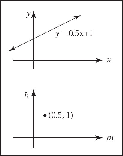
The set of points on the line y = mx + b in (x, y) space can also be represented by a single point in (m, b) space so the top line and the bottom point represent the same geometric entity: a 2D line.

In angle-intercept space we parameterize the line by angle ϕ ∈ [−π/2, π/2) rather than slope.
dμ=cos ϕ dϕ db.
It can be shown that this measure, up to a constant, is the only one that is invariant with respect to rotation and translation.
This measure can be converted into an appropriate measure for other parameterizations of the line. For example, the appropriate measure for (m, b) space is
dμ=dm db(1+m2)32.
For the space of lines parameterized in (u, v) space,
ux+vy+1=0,
the appropriate measure is
dμ=du dv(u2+v2)32.
For lines parameterized in terms of (a, b), the x-intercept and y-intercept, the measure is
dμ=ab da db(a2+b2)32.
Note that any of those spaces are equally valid ways to specify lines, and which is best depends upon the circumstances. However, one might wonder whether there exists a coordinate system where the measure of a set of lines is just an area in the dual space. In fact, there is such a coordinate system, and it is delightfully simple; it is the normal coordinates which specify a line in terms of the normal distance from the origin to the line, and the angle the normal of the line makes with respect to the x-axis (Figure 14.5). The implicit equation for such lines is
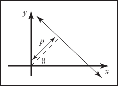
The normal coordinates of a line use the normal distance to the origin and an angle to specify a line.
x cos θ+ysin θ−p=0.
And, indeed, the measure in that space is
dμ=dp dθ.
We shall use these measures to choose fair random lines in a later section.
14.1.3 Example: Measure of Lines in 3D
In 3D there are many ways to parameterize lines. Perhaps, the simplest way is to use their intersection with a particular plane along with some specification of their orientation. For example, we could chart the intersection with the xy plane along with the spherical coordinates of its orientation. Thus, each line would be specified as a (x, y, θ, ϕ) quadruple. This shows that lines in 3D are 4D entities, i.e., they can be described as points in a 4D space.
The differential measure of a line should not vary with (x, y), but bundles of lines with equal cross section should have equal measure. Thus, a fair differential measure is
Another way to parameterize lines is to chart the intersection with two parallel planes. For example, if the line intersects the plane z = 0 at (x = u, y = v) and the plane z = 1 at (x = s, y = t), then the line can be described by the quadruple (u, v, s, t). Note, that like the previous parameterization, this one is degenerate for lines parallel to the xy plane. The differential measure is more complicated for this parameterization although it can be approximated as
dμ≈du dv a ds dt,
for bundles of lines nearly parallel to the z-axis. This is the measure often implicitly used in image-based rendering.
For sets of lines that intersect a sphere, we can use the parameterization of the two points where the line intersects the sphere. If these are in spherical coordinates, then the point can be described by the quadruple (θ1, ϕ1, θ2, ϕ2) and the measure is just the differential area associated with each point:
dμ=sin θ1 dθ1 dϕ1 sin θ2 dθ2 dϕ2.
This implies that picking two uniform random endpoints on the sphere results in a line with uniform density. This observation was used to compute form-factors by Mateu Sbert in his dissertation (Sbert, 1997).
Note that sometimes we want to parameterize directed lines, and sometimes we want the order of the endpoints not to matter. This is a bookkeeping detail that is especially important for rendering applications where the amount of light flowing along a line is different in the two directions along the line.
14.2 Continuous Probability
Many graphics algorithms use probability to construct random samples to solve integration and averaging problems. This is the domain of applied continuous probability which has basic connections to measure theory.
14.2.1 One-Dimensional Continuous Probability Density Functions
Loosely speaking, a continuous random variable x is a scalar or vector quantity that “randomly” takes on some value from the real line ℝ = (−∞, +∞). The behavior of x is entirely described by the distribution of values it takes. This distribution of values can be quantitatively described by the probability density function (pdf), p, associated with x (the relationship is denoted x ∼ p). The probability that x assumes a particular value in some interval [a, b] is given by the following integral:
Probability(x∈[a,b])=∫bap(x)dx. (14.1)
Loosely speaking, the probability density function p describes the relative likelihood of a random variable taking a certain value; if p(x1) = 6.0 andp(x2) = 3.0, then a random variable with density p is twice as likely to have a value “near” x1 than it is to have a value near x2. The density p has two characteristics:
p(x)≥0 (probability is nonnegative), (14.2)
∫+∞−∞p(x)dx=1 (Probability(x∈ℝ)=1). (14.3)
As an example, the canonical random variable ξ takes on values between zero (inclusive) and one (non-inclusive) with uniform probability (here uniform simply means each value for ξ is equally likely). This implies that the probability density function q for ξ is
q(ξ)={1if 0 ≤ ξ < 1,0otherwise,
The space over which ξ is defined is simply the interval [0,1). The probability that ξ takes on a value in a certain interval [a, b] ∈ [0,1) is
Probability(a≤ξ≤b)=∫ba1 dx=b−a.
14.2.2 One-Dimensional Expected Value
The average value that a real function f of a one-dimensional random variable with underlying pdf p will take on is called its expected value, E(f(x)) (sometimes written Ef(x)):
E(f(x))=∫f(x)p(x)dx.
The expected value of a one-dimensional random variable can be calculated by setting f(x) = x. The expected value has a surprising and useful property: the expected value of the sum of two random variables is the sum of the expected values of those variables:
E(x+y)=E(x)+E(y),
for random variables x and y. Because functions of random variables are themselves random variables, this linearity of expectation applies to them as well:
E(f(x)+g(y))=E(f(x))+E(g(y)).
An obvious question to ask is whether this property holds if the random variables being summed are correlated (variables that are not correlated are called independent). This linearity property in fact does hold whether or not the variables are independent! This summation property is vital for most Monte Carlo applications.
14.2.3 Multidimensional Random Variables
The discussion of random variables and their expected values extends naturally to multidimensional spaces. Most graphics problems will be in such higher-dimensional spaces. For example, many lighting problems are phrased on the surface of the hemisphere. Fortunately, if we define a measure μ on the space the random variables occupy, everything is very similar to the one-dimensional case. Suppose the space S has associated measure μ; for example S is the surface of a sphere and μ measures area. We can define a pdf p : S ↦ ℝ, and if x is a random variable with x ∼ p, then the probability that x will take on a value in some region Si ⊂ S is given by the integral
Probability(x∈Si)=∫Sip(x)dμ.
Here Probability (event) is the probability that event is true, so the integral is the probability that x takes on a value in the region Si.
In graphics, S is often an area (dμ = dA = dxdy) or a set of directions (points on a unit sphere: dμ = dω = sinθ dθ dϕ). As an example, a two-dimensional random variable α is a uniformly distributed random variable on a disk of radius R. Here uniformly means uniform with respect to area, e.g., the way a bad dart player’s hits would be distributed on a dart board. Since it is uniform, we know that p(α) is some constant. From the fact that the area of the disk is πr2 and that the total probability is one, we can deduce that
This means that the probability that α is in a certain subset S1 of the disk is just
Probability(α∈S1)=∫S11πR2dA.
This is all very abstract. To actually use this information, we need the integral in a form we can evaluate. Suppose Si is the portion of the disk closer to the center than the perimeter. If we convert to polar coordinates, then α is represented as a (r, ϕ) pair, and S1 is the region where r < R/2. Note, that just because α is uniform, it does not imply that ϕ or r are necessarily uniform (in fact, ϕ is uniform, and r is not uniform). The differential area dA is just r dr dϕ. Thus,
Probability(r<R2)=∫2π0∫R201πR2r dr dϕ=0.25.
The formula for expected value of a real function applies to the multidimensional case:
E(f(x))=∫Sf(x)p(x)dμ,
where x ∈ S and f : S ↦ ℝ, and p : S ↦ ℝ. For example, on the unit square S = [0,1] × [0,1] and p(x, y) = 4xy, the expected value of the x coordinate for (x, y) ∼ p is
E(x)= ∫Sf(x,y)p(x,y)dA= ∫10∫104x2y dx dy= 23.
Note that here f(x, y) = x.
14.2.4 Variance
The variance, V(x), of a one-dimensional random variable is, by definition, the expected value of the square of the difference between x and E(x):
V(x)≡E([x−E(x)]2).
Some algebraic manipulation gives the non-obvious expression:
The expression E([x — E(x)]2) is more useful for thinking intuitively about vari-ance, while the algebraically equivalent expression E(x2) — [E(x)]2 is usually convenient for calculations. The variance of a sum of random variables is the sum of the variances if the variables are independent. This summation property of variance is one of the reasons it is frequently used in analysis of probabilistic models. The square root of the variance is called the standard deviation, σ, which gives some indication of expected absolute deviation from the expected value.
14.2.5 Estimated Means
Many problems involve sums of independent random variables xi, where the variables share a common density p. Such variables are said to be independent identically distributed (iid) random variables. When the sum is divided by the number of variables, we get an estimate of E(x):
As N increases, the variance of this estimate decreases. We want N to be large enough so that we have confidence that the estimate is “close enough.” However, there are no sure things in Monte Carlo; we just gain statistical confidence that our estimate is good. To be sure, we would have to have N = ∞. This confidence is expressed by the Law of Large Numbers:
14.3 Monte Carlo Integration
In this section, the basic Monte Carlo solution methods for definite integrals are outlined. These techniques are then straightforwardly applied to certain integral problems. All of the basic material of this section is also covered in several of the classic Monte Carlo texts. (See the Notes section at the end of this chapter.)
As discussed earlier, given a function f : S ↦ ℝ and a random variable x ∼ p, we can approximate the expected value of f(x) by a sum:
Because the expected value can be expressed as an integral, the integral is also approximated by the sum. The form of Equation (14.4) is a bit awkward; we would usually like to approximate an integral of a single function g rather than a product fp. We can accomplish this by substituting g = fp as the integrand:
For this formula to be valid, p must be positive when g is nonzero.
So to get a good estimate, we want as many samples as possible, and we want the g/p to have a low variance (g and p should have a similar shape). Choosing p intelligently is called importance sampling, because if p is large where g is large, there will be more samples in important regions. Equation (14.4) also shows the fundamental problem with Monte Carlo integration: diminishing return. Because the variance of the estimate is proportional to 1/N, the standard deviation is proportional to . Since the error in the estimate behaves similarly to the standard deviation, we will need to quadruple N to halve the error.
Another way to reduce variance is to partition S, the domain of the integral, into several smaller domains Si, and evaluate the integral as a sum of integrals over the Si. This is called stratified sampling, the technique that jittering employs in pixel sampling (Chapter 4). Normally only one sample is taken in each Si (with density pi), and in this case the variance of the estimate is:
It can be shown that the variance of stratified sampling is never higher than unstratified if all strata have equal measure:
The most common example of stratified sampling in graphics is jittering for pixel sampling as discussed in Section 13.4.
As an example of the Monte Carlo solution of an integral I, set g(x) equal to x over the interval (0,4):
The impact of the shape of the function p on the variance of the N sample estimates is shown in Table 14.1. Note that the variance is reduced when the shape of p is similar to the shape of g. The variance drops to zero if p = g/I, but I is not usually known or we would not have to resort to Monte Carlo. One important principle illustrated in Table 14.1 is that stratified sampling is often far superior to importance sampling (Mitchell, 1996). Although the variance for this stratification on I is inversely proportional to the cube of the number of samples, there is no general result for the behavior of variance under stratification. There are some functions for which stratification does no good. One example is a white noise function, where the variance is constant for all regions. On the other hand, most functions will benefit from stratified sampling, because the variance in each subcell will usually be smaller than the variance of the entire domain.
Variance for Monte Carlo estimate of .
Method |
Sampling function |
Variance |
Samples needed for standard error of 0.008 |
|---|---|---|---|
importance |
(6 – x)/(16) |
56.8N−1 |
887,500 |
importance |
1/4 |
21.3N−1 |
332,812 |
importance |
(x + 2)/16 |
6.3N−1 |
98,437 |
importance |
x/8 |
0 |
1 |
stratified |
1/4 |
21.3Nx−3 |
70 |
14.3.1 Quasi—Monte Carlo Integration
A popular method for quadrature is to replace the random points in Monte Carlo integration with quasi-random points. Such points are deterministic, but are in some sense uniform. For example, on the unit square [0, 1]2, a set of N quasi-random points should have the following property on a region of area A within the square:
For example, a set of regular samples in a lattice has this property.
Quasi-random points can improve performance in many integration applications. Sometimes care must be taken to make sure that they do not introduce aliasing. It is especially nice that, in any application where calls are made to random or stratified points in [0, 1]d, one can substitute d-dimensional quasi-random points with no other changes.
The key intuition motivating quasi—Monte Carlo integration is that when estimating the average value of an integrand, any set of sample points will do, provided they are “fair.”
14.4 Choosing Random Points
We often want to generate sets of random or pseudorandom points on the unit square for applications such as distribution ray tracing. There are several methods for doing this, e.g., jittering (see Section 13.4). These methods give us a set of N reasonably equidistributed points on the unit square [0, 1]2 : (u1, v1) through (uN , vN).
Sometimes, our sampling space may not be square (e.g., a circular lens), or may not be uniform (e.g., a filter function centered on a pixel). It would be nice if we could write a mathematical transformation that would take our equidistributed points (ui, vi) as input and output a set of points in our desired sampling space with our desired density. For example, to sample a camera lens, the transformation would take (ui, vi) and output (ri, ϕi) such that the new points are approximately equidistributed on the disk of the lens. While we might be tempted to use the transform
it has a serious problem. While the points do cover the lens, they do so nonuniformly (Figure 14.6). What we need in this case is a transformation that takes equal-area regions to equal-area regions—one that takes uniform sampling distributions on the square to uniform distributions on the new domain.

The transform that takes the horizontal and vertical dimensions uniformly to (r, ϕ) does not preserve relative area; not all of the resulting areas are the same.
There are several ways to generate such nonuniform points or uniform points on non-rectangular domains, and the following sections review the three most often used: function inversion, rejection, and Metropolis.
14.4.1 Function Inversion
If the density f(x) is one-dimensional and defined over the interval x ∈ [xmin, xmax], then we can generate random numbers αi that have density f from a set of uniform random numbers ξi, where ξi ∈ [0,1]. To do this, we need the cumulative probability distribution function P(x):
To get αi, we simply transform ξi :
where P−1 is the inverse of P. If P is not analytically invertible, then numerical methods will suffice, because an inverse exists for all valid probability distribution functions.
Note that analytically inverting a function is more confusing than it should be due to notation. For example, if we have the function
for x > 0, then the inverse function is expressed in terms of y as a function of x:
When the function is analytically invertible, it is almost always that simple. However, things are a little more opaque with the standard notation:
Here x is just a dummy variable. You may find it easier to use the less standard notation:
while keeping in mind that these are inverse functions of each other.
For example, to choose random points xi that have density
on [−1,1], we see that
and
so we can “warp” a set of canonical random numbers (ξ1, ... , ξN) to the properly distributed numbers
Of course, this same warping function can be used to transform “uniform” jittered samples into nicely distributed samples with the desired density.
If we have a random variable α = (αx, αy) with two-dimensional density (x, y) defined on [xmin, xmax] × [ymin, ymax], then we need the two-dimensional distribution function:
We first choose an xi using the marginal distribution F(x, ymax) and then choose yi according to F(xi,y)/F(xi,ymax). If f(x,y) is separable (expressible as g(x)h(y)), then the one-dimensional techniques can be used on each dimension.
Returning to our earlier example, suppose we are sampling uniformly from the disk of radius R, so p(r, ϕ) = 1/(πR2). The two-dimensional distribution function is
This means that a canonical pair (ξ1, ξ2) can be transformed to a uniform random point on the disk:
This mapping is shown in Figure 14.7.

A mapping that takes equal area regions in the unit square to equal area regions in the disk.
To choose reflected ray directions for some realistic rendering applications, we choose points on the unit hemisphere according to the density:
where n is a Phong-like exponent, θ is the angle from the surface normal and θ ∈ [0, π/2] (is on the upper hemisphere) and ϕ is the azimuthal angle (ϕ ∈ [0, 2π]). The cumulative distribution function is
The sin θ′ term arises because, on the sphere, dω = cos θdθdϕ. When the marginal densities are found, p (as expected) is separable, and we find that a (ξ1 , ξ2) pair of canonical random numbers can be transformed to a direction by
Again, a nice thing about this is that a set of jittered points on the unit square can be easily transformed to a set of jittered points on the hemisphere with the desired distribution. Note that if n is set to 1, we have a diffuse distribution, as is often needed.
Often we must map the point on the sphere into an appropriate direction with respect to a uvw basis. To do this, we can first convert the angles to a unit vector :
As an efficiency improvement, we can avoid taking trigonometric functions of inverse trigonometric functions (e.g., cos (arccos θ)). For example, when n = 1 (a diffuse distribution), the vector a simplifies to
14.4.2 Rejection
A rejection method chooses points according to some simple distribution and rejects some of them that are in a more complex distribution. There are several scenarios where rejection is used, and we show some of these by example.
Suppose we want uniform random points within the unit circle. We can first choose uniform random points (x, y) ∈ [−1,1]2 and reject those outside the circle. If the function r() returns a canonical random number, then the procedure is:
done = false
while (not done) do
x = −1 + 2r()
y = − 1 + 2r()
if (x2 + y2 < 1) then
done = true
If we want a random number x ∼ p and we know that p : [a, b] ↦ ℝ, and that for all x, p(x) < m, then we can generate random points in the rectangle [a, b] × [0, m] and take those where y < p(x):
done = false
while (not done) do
x = a + r()(b - a)
y = r()m
if (y < p(x)) then
done = true
This same idea can be applied to take random points on the surface of a sphere. To pick a random unit vector with uniform directional distribution, we first pick a random point in the unit sphere and then treat that point as a direction vector by taking the unit vector in the same direction:
done = false
while (not done) do
x = −1 + 2r()
y = −1 + 2r()
z = −1 + 2r()
if ((l = ) < 1) then
done = true
x = x/l
y = y/l
z = z/l
Although the rejection method is usually simple to code, it is rarely compatible with stratification. For this reason, it tends to converge more slowly and should thus be used mainly for debugging, or in particularly difficult circumstances.
14.4.3 Metropolis
The Metropolis method uses random mutations to produce a set of samples with a desired density. This concept is used extensively in the Metropolis Light Transport algorithm referenced in the chapter notes. Suppose we have a random point x0 in a domain S. Further, suppose for any point x, we have a way to generate random y ∼ px. We use the marginal notation px(y) ≡ p(x → y) to denote this density function. Now, suppose we let x1 be a random point in S selected with underlying density p(x0 → x1). We generate x2 with density p(x1 → x0) and so on. In the limit, where we generate an infinite number of samples, it can be proved that the samples will have some underlying density determined by p regardless of the initial point x0.
Now, suppose we want to choose p such that the underlying density of samples to which we converge is proportional to a function f(x) where f is a nonnegative function with domain S. Further, suppose we can evaluate f, but we have little or no additional knowledge about its properties (such functions are common in graphics). Also, suppose we have the ability to make “transitions” from xi to xi+1 with underlying density function t(xi → xi+1). To add flexibility, further suppose we add the potentially nonzero probability that xi transitions to itself, i.e., xi+1 = xi. We phrase this as generating a potential candidate y ∼ t(xi → y) and “accepting” this candidate (i.e.,xi+1 = y) with probability a(xi → y) and rejecting it (i.e., xi+1 = xi) with probability 1 − a(xi → y). Note that the sequence x0, x1, x2, ... will be a random set, but there will be some correlation among samples. They will still be suitable for Monte Carlo integration or density estimation, but analyzing the variance of those estimates is much more challenging.
Now, suppose we are given a transition function t(x → y) and a function f(x) of which we want to mimic the distribution, can we use a(y → x) such that the points are distributed in the shape of f ? Or more precisely,
It turns out this can be forced by making sure the xi are stationary in some strong sense. If you visualize a huge collection of sample points x, you want the “flow” between two points to be the same in each direction. If we assume the density of points near x and y are proportional to f(x) and f(y), respectively, then the flow in the two directions should be the same:
where k is some positive constant. Setting these two flows constant gives a constraint on a:
Thus, if either a(y → x) or a(x → y) is known, so is the other. Making them larger improves the chance of acceptance, so the usual technique is to set the larger of the two to 1.
A difficulty in using the Metropolis sample generation technique is that it is hard to estimate how many points are needed before the set of points is “good.” Things are accelerated if the first n points are discarded, although choosing n wisely is nontrivial.
14.4.4 Example: Choosing Random Lines in the Square
As an example of the full process of designing a sampling strategy, consider the problem of finding random lines that intersect the unit square [0,1]2. We want this process to be fair; that is, we would like the lines to be uniformly distributed within the square. Intuitively, we can see that there is some subtlety to this problem; there are “more” lines at an oblique angle than in horizontal or vertical directions. This is because the cross section of the square is not uniform.
Our first goal is to find a function-inversion method, if one exists, and then to fall back on rejection or Metropolis if that fails. This is because we would like to have stratified samples in line space. We try using normal coordinates first, because the problem of choosing random lines in the square is just the problem of finding uniform random points in whatever part of (r, θ) space corresponds to lines in the square.
Consider the region where −π/2 < θ < 0. What values of r correspond to lines that hit the square? For those angles, r < cos θ are all the lines that hit the square as shown in Figure 14.8. Similar reasoning in the other four quadrants finds the region in (r, θ) space that must be sampled, as shown in Figure 14.9. The equation of the boundary of that region rmax(θ)is
![Figure showing the largest distance r corresponds to a line hitting the square for θ ∈ [−π/2, 0]. Because the square has sidelength one, r = cos θ.](http://images-20200215.ebookreading.net/23/1/1/9781482229417/9781482229417__fundamentals-of-computer__9781482229417__image__fig14-8.png)
The largest distance r corresponds to a line hitting the square for θ ∈ [−π/2, 0]. Because the square has sidelength one, r = cos θ.
![Figure showing the maximum radius for lines hitting the unit square [0,1]2 as a function of θ.](http://images-20200215.ebookreading.net/23/1/1/9781482229417/9781482229417__fundamentals-of-computer__9781482229417__image__fig14-9.png)
Because the region under rmax(θ) is a simple function bounded below by r = 0, we can sample it by first choosing θ according to the density function:
The denominator here is 4. Now, we can compute the cumulative probability distribution function:
We can invert this by manipulating ξ1 = P(θ) into the form θ = g(ξ1). This yields
Once we have θ, then r is simply:
As discussed earlier, there are many parameterizations of the line, and each has an associated “fair” measure. We can generate random lines in any of these spaces as well. For example, in slope-intercept space, the region that hits the square is shown in Figure 14.10. By similar reasoning to the normal space, the density function for the slope is
![Figure showing the region of (m,b) space that contains lines that intersect the unit square [0,1]2.](http://images-20200215.ebookreading.net/23/1/1/9781482229417/9781482229417__fundamentals-of-computer__9781482229417__image__fig14-10.png)
with respect to the differential measure
This gives rise to the cumulative distribution function:
These can be inverted by solving two quadratic equations. Given an m generated using ξ1, we then have
This is not a better way than using normal coordinates; it is just an alternative way.
Frequently Asked Questions
This chapter discussed probability but not statistics. What is the distinction?
Probability is the study of how likely an event is. Statistics infers characteristics of large, but finite, populations of random variables. In that sense, statistics could be viewed as a specific type of applied probability.
Is Metropolis sampling the same as the Metropolis Light Transport Algorithm?
No. The Metropolis Light Transport (Veach & Guibas, 1997) algorithm uses Metropolis sampling as part of its procedure, but it is specifically for rendering, and it has other steps as well.
Notes
The classic reference for geometric probability is Geometric Probability (Solomon, 1978). Another method for picking random edges in a square is given in Random-Edge Discrepancy of Supersampling Patterns (Dobkin & Mitchell, 1993). More information on quasi-Monte Carlo methods for graphics can be found in Efficient Multidimensional Sampling (Kollig & Keller, 2002). Three classic and very readable books on Monte Carlo methods are Monte Carlo Methods (Hammersley & Handscomb, 1964), Monte Carlo Methods, Basics (Kalos & Whitlock, 1986), and The Monte Carlo Method (Sobel, Stone, & Messer, 1975).
Exercises
- What is the average value of the function xyz in the unit cube (x, y, z) ∈ [0, 1]3?
- What is the average value of r on the unit-radius disk: (r, ϕ) ∈ [0,1] × [0, 2π)?
- Show that the uniform mapping of canonical random points (ξ1, ξ2) to the barycentric coordinates of any triangle is: β = 1 − , and γ = (1 − u)ξ2.
- What is the average length of a line inside the unit square? Verify your answer by generating ten million random lines in the unit square and averaging their lengths.
- What is the average length of a line inside the unit cube? Verify your answer by generating ten million random lines in the unit cube and averaging their lengths.
- Show from the definition of variance that V(x) = E(x2) − [E(x)]2.