Chapter 21

Tone Reproduction

Erik Reinhard

As discussed in Chapter 20, the human visual system adapts to a wide range of viewing conditions. Under normal viewing, we may discern a range of around 4 to 5 log units of illumination, i.e., the ratio between brightest and darkest areas where we can see detail may be as large as 100,000 : 1. Through adaptation processes, we may adapt to an even larger range of illumination. We call images that are matched to the capabilities of the human visual system high dynamic range.

Visual simulations routinely produce images with a high dynamic range (Ward Larson & Shakespeare, 1998). Recent developments in image-capturing techniques allow multiple exposures to be aligned and recombined into a single high dynamic range image (Debevec & Malik, 1997). Multiple exposure techniques are also available for video. In addition, we expect future hardware to be able to photograph or film high dynamic range scenes directly. In general, we may think of each pixel as a triplet of three floating point numbers.

As it is becoming easier to create high dynamic range imagery, the need to display such data is rapidly increasing. Unfortunately, most current display devices, monitors and printers, are only capable of displaying around 2 log units of dynamic range. We consider such devices to be of low dynamic range. Most images in existence today are represented with a byte-per-pixel-per-color channel, which is matched to current display devices, rather than to the scenes they represent.

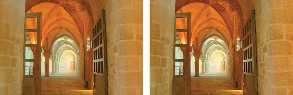
Typically, low dynamic range images are not able to represent scenes without loss of information. A common example is an indoor room with an outdoor area visible through the window. Humans are easily able to see details of both the indoor part and the outside part. A conventional photograph typically does not capture this full range of information—the photographer has to choose whether the indoor or the outdoor part of the scene is properly exposed (see Figure 21.1). These decisions may be avoided by using high dynamic range imaging and preparing these images for display using techniques described in this chapter (see Figure 21.2).

There are two strategies available to display high dynamic range images. First, we may develop display devices which can directly accommodate a high dynamic range (Seetzen, Whitehead, & Ward, 2003; Seetzen et al., 2004). Second, we may prepare high dynamic range images for display on low dynamic range display devices (Upstill, 1985). This is currently the more common approach and the topic of this chapter. Although we foresee that high dynamic range display devices will become widely used in the (near) future, the need to compress the dynamic range of an image may diminish, but will not disappear. In particular, printed media such as this book are, by their very nature, low dynamic range.

Compressing the range of values of an image for the purpose of display on a low dynamic range display device is called tonemapping or tone reproduction. A simple compression function would be to normalize an image (see Figure 21.3 (left)). This constitutes a linear scaling which tends to be sufficient only if the dynamic range of the image is only marginally higher than the dynamic range of the display device. For images with a higher dynamic range, small intensity differences will be quantized to the same display value such that visible details are lost. In Figure 21.3 (middle) all pixel values larger than a user-specified maximum are set to this maximum (i.e., they are clamped). This makes the normalization less dependent on noisy outliers, but here we lose information in the bright areas of the image. For comparison, Figure 21.3 (right) is a tonemapped version showing detail in both the dark and the bright regions.

In general, linear scaling will not be appropriate for tone reproduction. The key issue in tone reproduction is then to compress an image while at the same time preserving one or more attributes of the image. Different tone reproduction algorithms focus on different attributes such as contrast, visible detail, brightness, or appearance.

Ideally, displaying a tonemapped image on a low dynamic range display device would create the same visual response in the observer as the original scene. Given the limitations of display devices, this will not be achievable, although we could aim for approximating this goal as closely as possible.

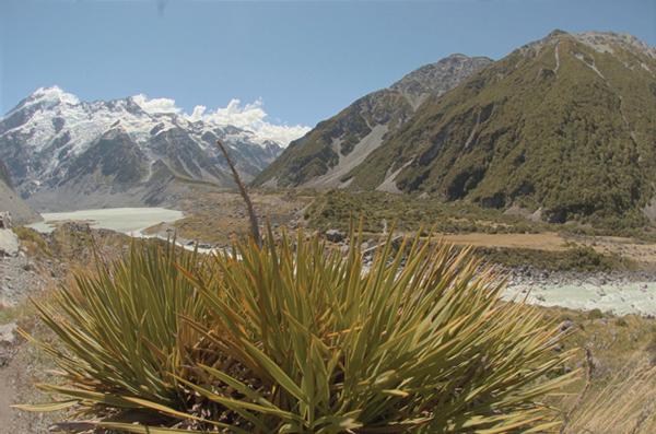
As an example, we created the high dynamic range image shown in Figure 21.4. This image was then tonemapped and displayed on a display device. The display device itself was then placed in the scene such that it displays its own background (Figure 21.5). In the ideal case, the display should appear transparent. Dependent on the quality of the tone reproduction operator, as well as the nature of the scene being depicted, this goal may be more or less achievable.

21.1 Classification

Although it would be possible to classify tone reproduction operators by which attribute they aim to preserve, or for which task they were developed, we classify algorithms according to their general technique. This will enable us to show the differences and similarities between a significant number of different operators, and so, hopefully, contribute to the meaningful selection of specific operators for given tone reproduction tasks.

The main classification scheme we follow hinges upon the realization that tone reproduction operators are based on insights gained from various disciplines. In particular, several operators are based on knowledge of human visual perception.

The human visual system detects light using photoreceptors located in the retina. Light is converted to an electrical signal which is partially processed in the retina and then transmitted to the brain. Except for the first few layers of cells in the retina, the signal derived from detected light is transmitted using impulse trains. The information-carrying quantity is the frequency with which these electrical pulses occur.

The range of light that the human visual system can detect is much larger than the range of frequencies employed by the human brain to transmit information. Thus, the human visual system effortlessly solves the tone reproduction problem—a large range of luminances is transformed into a small range of frequencies of impulse trains. Emulating relevant aspects of the human visual system is therefore a worthwhile approach to tone reproduction; this approach is explained in more detail in Section 21.7.

A second class of operators is grounded in physics. Light interacts with surfaces and volumes before being absorbed by the photoreceptors. In computer graphics, light interaction is generally modeled by the rendering equation. For purely diffuse surfaces, this equation may be simplified to the product between light incident upon a surface (illuminance), and this surface’s ability to reflect light (reflectance) (Oppenheim, Schafer, & Stockham, 1968).

Since reflectance is a passive property of surfaces, for diffuse surfaces it is, by definition, low dynamic range—typically between 0.005 and 1 (Stockham, 1972). The reflectance of a surface cannot be larger than 1, since then it would reflect more light than was incident upon the surface. Illuminance, on the other hand, can produce arbitrarily large values and is limited only by the intensity and proximity of the light sources.

The dynamic range of an image is thus predominantly governed by the illuminance component. In the face of diffuse scenes, a viable approach to tone reproduction may therefore be to separate reflectance from illuminance, compress the illuminance component, and then recombine the image.

However, the assumption that all surfaces in a scene are diffuse is generally incorrect. Many high dynamic range images depict highlights and/or directly visible light sources (Figure 21.3). The luminance reflected by a specular surface may be almost as high as the light source it reflects.

Various tone reproduction operators currently used split the image into a high dynamic range base layer and a low dynamic range detail layer. These layers would represent illuminance and reflectance if the depicted scene were entirely diffuse. For scenes containing directly visible light sources or specular highlights, separation into base and detail layers still allows the design of effective tone reproduction operators, although no direct meaning can be attached to the separate layers. Such operators are discussed in Section 21.5.

21.2 Dynamic Range

Conventional images are stored with one byte per pixel for each of the red, green and blue components. The dynamic range afforded by such an encoding depends on the ratio between smallest and largest representable value, as well as the step size between successive values. Thus, for low dynamic range images, there are only 256 different values per color channel.

High dynamic range images encode a significantly larger set of possible values; the maximum representable value may be much larger and the step size between successive values may be much smaller. The file size of high dynamic range images is therefore generally larger as well, although at least one standard (the OpenEXR high dynamic range file format (Kainz, Bogart, & Hess, 2003)) includes a very capable compression scheme.

A different approach to limit file sizes is to apply a tone reproduction operator to the high dynamic data. The result may then be encoded in JPEG format. In addition, the input image may be divided pixel-wise by the tonemapped image. The result of this division can then be subsampled and stored as a small amount of data in the header of the same JPEG image (G. Ward & Simmons, 2004). The file size of such sub-band encoded images is of the same order as conventional JPEG encoded images. Display programs can display the JPEG image directly or may reconstruct the high dynamic range image by multiplying the tonemapped image with the data stored in the header.

In general, the combination of smallest step size and ratio of the smallest and largest representable values determines the dynamic range that an image encoding scheme affords. For computer-generated imagery, an image is typically stored as a triplet of floating point values before it is written to file or displayed on screen, although more efficient encoding schemes are possible (Reinhard, Ward, Debevec, & Pattanaik, 2005). Since most display devices are still fitted with eight-bit D/A converters, we may think of tone reproduction as the mapping of floating point numbers to bytes such that the result is displayable on a low dynamic range display device.

The dynamic range of individual images is generally smaller, and is determined by the smallest and largest luminances found in the scene. A simplistic approach to measure the dynamic range of an image may therefore compute the ratio between the largest and smallest pixel value of an image. Sensitivity to outliers may be reduced by ignoring a small percentage of the darkest and brightest pixels.

Alternatively, the same ratio may be expressed as a difference in the logarithmic domain. This measure is less sensitive to outliers. The images shown in the margin on this page are examples of images with different dynamic ranges. Note that the night scene in this case does not have a smaller dynamic range than the day scene. While all the values in the night scene are smaller, the ratio between largest and smallest values is not.

However, the recording device or rendering algorithm may introduce noise which will lower the useful dynamic range. Thus, a measurement of the dynamic range of an image should factor in noise. A better measure of dynamic range would therefore be a signal-to-noise ratio, expressed in decibels, as used in signal processing.

21.3 Color

Tone reproduction operators normally compress luminance values, rather than work directly on the red, green, and blue components of a color image. After these luminance values have been compressed into display values Ld(x,y), a color image may be reconstructed by keeping the ratios between color channels the same as they were before compression (using s = 1) (Schlick, 1994b):

$\begin{array}{c}{I}_{r,d}\left(x,y\right)={\left(\frac{I_r\left(x,y\right)}{L_v\left(x,y\right)}\right)}^s{L}_d\left(x,y\right),\\ I_{g,d}\left(x,y\right)={\left(\frac{I_g\left(x,y\right)}{L_v\left(x,y\right)}\right)}^s{L}_d\left(x,y\right),\\ I_{b,d}\left(x,y\right)={\left(\frac{I_b\left(x,y\right)}{L_v\left(x,y\right)}\right)}^s{L}_d\left(x,y\right).\end{array}$

The results frequently appear over-saturated, because human color perception is nonlinear with respect to overall luminance level. This means that if we view an image of a bright outdoor scene on a monitor in a dim environment, our eyes are adapted to the dim environment rather than the outdoor lighting. By keeping color ratios constant, we do not take this effect into account.

Alternatively, the saturation constant s may be chosen smaller than one. Such per-channel gamma correction may desaturate the results to an appropriate level, as shown in Figure 21.11 (Fattal, Lischinski, & Werman, 2002). A more comprehensive solution is to incorporate ideas from the field of color appearance modeling into tone reproduction operators (Pattanaik, Ferwerda, Fairchild, & Green-berg, 1998; Fairchild & Johnson, 2004; Reinhard & Devlin, 2005).

Finally, if an example image with a representative color scheme is already available, this color scheme may be applied to a new image. Such a mapping of colors between images may be used for subtle color correction, such as saturation adjustment or for more creative color mappings. The mapping proceeds by converting both source and target images to a decorrelated color space. In such a color space, the pixel values in each color channel may be treated independently without introducing too many artifacts (Reinhard, Ashikhmin, Gooch, & Shirley, 2001).

Mapping colors from one image to another in a decorrelated color space is then straightforward: compute the mean and standard deviation of all pixels in the source and target images for the three color channels separately. Then, shift and scale the target image so that in each color channel the mean and standard deviation of the target image is the same as the source image. The resulting image is then obtained by converting from the decorrelated color space to RGB and clamping negative pixels to zero. The dynamic range of the image may have changed as a result of applying this algorithm. It is therefore recommended to apply this algorithm on high dynamic range images and apply a conventional tone reproduction algorithm afterward. A suitable decorrelated color space is the opponent space from Section 19.2.4.

The result of applying such a color transform to the image in Figure 21.12 is shown in Figure 21.13.

21.4 Image Formation

For now, we assume that an image is formed as the result of light being diffusely reflected off of surfaces. Later in this chapter, we relax this constraint to scenes directly depicting light sources and highlights. The luminance Lv of each pixel is then approximated by the following product:

$L_v\left(x,y\right)=r\left(x,y\right)E_v\left(x,y\right).$

Here, r denotes the reflectance of a surface, and Ev denotes the illuminance. The subscript v indicates that we are using photometrically weighted quantities. Alternatively, we may write this expression in the logarithmic domain (Oppenheim et al., 1968):

$\begin{array}{cc}\hfill D\left(x,y\right)& =\log \left(L_v\left(x,y\right)\right)\hfill \\ \hfill & =\log \left(r\left(x,y\right)E_v\left(x,y\right)\right)\hfill \\ \hfill & =\log \left(r\left(x,y\right)\right)+\log \left(E_v\left(x,y\right)\right).\hfill \end{array}$

Photographic transparencies record images by varying the density of the material. In traditional photography, this variation has a logarithmic relation with luminance. Thus, in analogy with common practice in photography, we will use the term density representation (D) for log luminance. When represented in the log domain, reflectance and illuminance become additive. This facilitates separation of these two components, despite the fact that isolating either reflectance or illuminance is an under-constrained problem. In practice, separation is possible only to a certain degree and depends on the composition of the image. Nonetheless, tone reproduction could be based on disentangling these two components of image formation, as shown in the following two sections.

21.5 Frequency-Based Operators

For typical diffuse scenes, the reflectance component tends to exhibit high spatial frequencies due to textured surfaces as well as the presence of surface edges. On the other hand, illuminance tends to be a slowly varying function over space.

Since reflectance is low dynamic range and illuminance is high dynamic range, we may try to separate the two components. The frequency-dependence of both reflectance and illuminance provides a solution. We may, for instance, compute the Fourier transform of an image and attenuate only the low frequencies. This compresses the illuminance component while leaving the reflectance component largely unaffected—the very first digital tone reproduction operator known to us takes this approach (Oppenheim et al., 1968).

More recently, other operators have also followed this line of reasoning. In particular, bilateral and trilateral filters were used to separate an image into base and detail layers (Durand & Dorsey, 2002; Choudhury & Tumblin, 2003). Both filters are edge-preserving smoothing operators which may be used in a variety of different ways. Applying an edge-preserving smoothing operator to a density image results in a blurred image in which sharp edges remain present (Figure 21.14 (left)). We may view such an image as a base layer. If we then pixel-wise divide the high dynamic range image by the base layer, we obtain a detail layer which contains all the high-frequency detail (Figure 21.14 (right)).

For diffuse scenes, base and detail layers are similar to representations of illuminance and reflectance. For images depicting highlights and light sources, this parallel does not hold. However, separation of an image into base and detail layers is possible regardless of the image’s content. By compressing the base layer before recombining into a compressed density image, a low dynamic range density image may be created (Figure 21.15). After exponentiation, a displayable image is obtained.

Edge-preserving smoothing operators may also be used to compute a local adaptation level for each pixel, which may be used in a spatially varying or local tone reproduction operator. We describe this use of bilateral and trilateral filters in Section 21.7.

21.6 Gradient-Domain Operators

The arguments made for the frequency-based operators in the preceding section also hold for the gradient field. Assuming that no light sources are directly visible, the reflectance component will be a constant function with sharp spikes in the gradient field. Similarly, the illuminance component will cause small gradients everywhere.

Humans are generally able to separate illuminance from reflectance in typical scenes. The perception of surface reflectance after discounting the illuminant is called lightness. To assess the lightness of an image depicting only diffuse surfaces, B. K. P. Horn was the first to separate reflectance and illuminance using a gradient field (Horn, 1974). He used simple thresholding to remove all small gradients and then integrated the image, which involves solving a Poisson equation using the Full Multigrid Method (Press, Teukolsky, Vetterling, & Flannery, 1992).

The result is similar to an edge-preserving smoothing filter. This is according to expectation since Oppenheim’s frequency-based operator works under the same assumptions of scene reflectivity and image formation. In particular, Horn’s work was directly aimed at “mini-worlds of Mondrians,” which are simplified versions of diffuse scenes which resemble the abstract paintings by the famous Dutch painter Piet Mondrian.

Horn’s work cannot be employed directly as a tone reproduction operator, since most high dynamic range images depict light sources. However, a relatively small variation will turn this work into a suitable tone reproduction operator. If light sources or specular surfaces are depicted in the image, then large gradients will be associated with the edges of light sources and highlights. These cause the image to have a high dynamic range. An example is shown in Figure 21.16, where the highlights on the snooker balls cause sharp gradients.

We could therefore compress a high dynamic range image by attenuating large gradients, rather than thresholding the gradient field. This approach was taken by Fattal et al. who showed that high dynamic range imagery may be successfully compressed by integrating a compressed gradient field (Figure 21.17) (Fattal et al., 2002). Fattal’s gradient-domain compression is not limited to diffuse scenes.

21.7 Spatial Operators

In the following sections, we discuss tone reproduction operators which apply compression directly on pixels without transformation to other domains. Often global and local operators are distinguished. Tone reproduction operators in the former class change each pixel’s luminance values according to a compressive function which is the same for each pixel. The term global stems from the fact that many such functions need to be anchored to some values determined by analyzing the full image. In practice, most operators use the geometric average ${\overline{L}}_v$ to steer the compression:

${\overline{L}}_v=\text{exp}\left(\frac{\text{1}}{N}{\displaystyle \sum _{x,y}\log (\delta +L_v\left(x,y\right)}\right).\text{ (21.1)}$

In Equation (21.1), a small constant δ is introduced to prevent the average to become zero in the presence of black pixels. The geometric average is normally mapped to a predefined display value. The effect of mapping the geometric average to different display values is shown in Figure 21.18. Alternatively, sometimes the minimum or maximum image luminance is used. The main challenge faced in the design of a global operator lies in the choice of the compressive function.

On the other hand, local operators compress each pixel according to a specific compression function which is modulated by information derived from a selection of neighboring pixels, rather than the full image. The rationale is that a bright pixel in a bright neighborhood may be perceived differently than a bright pixel in a dim neighborhood. Design challenges in the development of a local operator involves choosing the compressive function, the size of the local neighborhood for each pixel, and the manner in which local pixel values are used. In general, local operators achieve better compression than global operators (Figure 21.19), albeit at a higher computational cost.

Both global and local operators are often inspired by the human visual system. Most operators employ one of two distinct compressive functions, which is orthogonal to the distinction between local and global operators. Display values Ld(x, y) are most commonly derived from image luminances Lv(x, y) by the following two functional forms:

$L_d\left(x,y\right)=\frac{L_v\left(x,y\right)}{f\left(x,y\right)},\text{ (21.2)}$

$L_d\left(x,y\right)=\frac{L_v\left(x,y\right)}{L_v\left(x,y\right)+f^n\left(x,y\right)}.\text{ (21.3)}$

In these equations, f(x, y) may either be a constant or a function which varies per pixel. In the former case, we have a global operator, whereas a spatially varying function f(x, y) results in a local operator. The exponent n is usually a constant which is fixed for a particular operator.

Equation (21.2) divides each pixel’s luminance by a value derived from either the full image or a local neighborhood. Equation (21.3) has an S-shaped curve on a log-linear plot and is called a sigmoid for that reason. This functional form fits data obtained from measuring the electrical response of photoreceptors to flashes of light in various species. In the following sections, we discuss both functional forms.

21.8 Division

Each pixel may be divided by a constant to bring the high dynamic range image within a displayable range. Such a division essentially constitutes linear scaling, as shown in Figure 21.3. While Figure 21.3 shows ad-hoc linear scaling, this approach may be refined by employing psychophysical data to derive the scaling constant f(x, y) = k in Equation (21.2) (G. J. Ward, 1994; Ferwerda, Pattanaik, Shirley, & Greenberg, 1996).

Alternatively, several approaches exist that compute a spatially varying divisor. In each of these cases, f(x, y) is a blurred version of the image, i.e., $f\left(x,y\right)=L_v^{\text{blur}}\left(x,y\right)$. The blur is achieved by convolving the image with a Gaussian filter (Chiu et al., 1993; Rahman, Jobson, & Woodell, 1996). In addition, the computation of f(x, y) by blurring the image may be combined with a shift in white point for the purpose of color appearance modeling (Fairchild & Johnson, 2002; G. M. Johnson & Fairchild, 2003; Fairchild & Johnson, 2004).

The size and the weight of the Gaussian filter has a profound impact on the resulting displayable image. The Gaussian filter has the effect of selecting a weighted local average. Tone reproduction is then a matter of dividing each pixel by its associated weighted local average. If the size of the filter kernel is chosen too small, then haloing artifacts will occur (Figure 21.20 (left)). Haloing is a common problem with local operators and is particularly evident when tone mapping relies on division.

In general, haloing artifacts may be minimized in this approach by making the filter kernel large (Figure 21.20 (right)). Reasonable results may be obtained by choosing a filter size of at least one quarter of the image. Sometimes even larger filter kernels are desirable to minimize artifacts. Note, that in the limit, the filter size becomes as large as the image itself. In that case, the local operator becomes global, and the extra compression normally afforded by a local approach is lost.

The functional form whereby each pixel is divided by a Gaussian-blurred pixel at the same spatial position thus requires an undesirable tradeoff between amount of compression and severity of artifacts.

21.9 Sigmoids

Equation (21.3) follows a different functional form from simple division, and, therefore, affords a different tradeoff between amount of compression, presence of artifacts, and speed of computation.

Sigmoids have several desirable properties. For very small luminance values, the mapping is approximately linear, so that contrast is preserved in dark areas of the image. The function has an asymptote at one, which means that the output mapping is always bounded between 0 and 1.

In Equation (21.3), the function f(x, y) may be computed as a global constant or as a spatially varying function. Following common practice in electro-physiology, we call f(x, y) the semi-saturation constant. Its value determines which values in the input image are optimally visible after tonemapping. In particular, if we assume that the exponent n equals 1, then luminance values equal to the semi-saturation constant will be mapped to 0.5. The effect of choosing different semi-saturation constants is shown in Figure 21.21.

The function f(x, y) may be computed in several different ways (Reinhard et al., 2005). In its simplest form, f(x, y) is set to ${\overline{L}}_v/k$, so that the geometric average is mapped to user parameter k (Figure 21.22) (Reinhard et al., 2002). In this case, a good initial value for k is 0.18, although for particularly bright or dark scenes this value may be raised or lowered. Its value may be estimated from the image itself (Reinhard, 2003). The exponent n in Equation (21.3) may be set to 1.

In this approach, the semi-saturation constant is a function of the geometric average, and the operator is therefore global. A variation of this global operator computes the semi-saturation constant by linearly interpolating between the geometric average and each pixel’s luminance:

$f\left(x,y\right)=a{L}_v\left(x,y\right)+\left(1-a\right){\overline{L}}_v.$

The interpolation is governed by user parameter a which has the effect of varying the amount of contrast in the displayable image (Figure 21.23) (Reinhard & Devlin, 2005). More contrast means less visible detail in the light and dark areas and vice versa. This interpolation may be viewed as a halfway house between a fully global and a fully local operator by interpolating between the two extremes without resorting to expensive blurring operations.

Although operators typically compress luminance values, this particular operator may be extended to include a simple form of chromatic adaptation. It thus presents an opportunity to adjust the level of saturation normally associated with tonemapping, as discussed at the beginning of this chapter.

Rather than compress the luminance channel only, sigmoidal compression is applied to each of the three color channels:

$\begin{array}{c}{I}_{r,d}\left(x,y\right)=\frac{I_r\left(x,y\right)}{I_r\left(x,y\right)+f^n\left(x,y\right)},\\ I_{g,d}\left(x,y\right)=\frac{I_g\left(x,y\right)}{I_g\left(x,y\right)+f^n\left(x,y\right)},\\ I_{b,d}\left(x,y\right)=\frac{I_b\left(x,y\right)}{I_b\left(x,y\right)+f^n\left(x,y\right)}.\end{array}$

The computation of f(x, y) is also modified to bilinearly interpolate between the geometric average luminance and pixel luminance and between each independent color channel and the pixel’s luminance value. We therefore compute the geometric average luminance value ${\overline{L}}_v$, as well as the geometric average of the red, green, and blue channels (${\overline{I}}_r,{\overline{I}}_g$, and ${\overline{I}}_b$). From these values, we compute f(x, y) for each pixel and for each color channel independently. We show the equation for the red channel (fr(x, y)):

$\begin{array}{cc}\hfill G_r\left(x,y\right)& =c{I}_r\left(x,y\right)+\left(1-c\right)L_v\left(x,y\right),\hfill \\ \hfill {\overline{G}}_r\left(x,y\right)& =c{\overline{I}}_r+\left(1-c\right){\overline{L}}_v,\hfill \\ \hfill f_r\left(x,y\right)& =a{G}_r\left(x,y\right)+\left(1-a\right){\overline{G}}_r\left(x,y\right).\hfill \end{array}$

The interpolation parameter a steers the amount of contrast as before, and the new interpolation parameter c allows a simple form of color correction (Figure 21.24).

So far we have not discussed the value of the exponent n in Equation (21.3). Studies in electrophysiology report values between n = 0.2 and n = 0.9 (Hood, Finkelstein, & Buckingham, 1979). While the exponent may be user-specified, for a wide variety of images we may estimate a reasonable value from the geometric average luminance ${\overline{L}}_v$ and the minimum and maximum luminance in the image (Lmin and Lmax) with the following empirical equation:

$n=0.3+0.7{\left(\frac{L_{\max }-{\overline{L}}_v}{L_{\max }-L_{\min }}\right)}^{1.4}.$

The several variants of sigmoidal compression shown so far are all global in nature. This has the advantage that they are fast to compute, and they are very suitable for medium to high dynamic range images. For very high dynamic range images, it may be necessary to resort to a local operator, since this may give some extra compression. A straightforward method to extend sigmoidal compression replaces the global semi-saturation constant by a spatially varying function, which may be computed in several different ways.

In other words, the function f(x, y) is so far assumed to be constant, but may also be computed as a spatially localized average. Perhaps the simplest way to accomplish this is to once more use a Gaussian-blurred image. Each pixel in a blurred image represents a locally averaged value which may be viewed as a suitable choice for the semi-saturation constant1.

As with division-based operators discussed in the previous section, we have to consider haloing artifacts. However, when an image is divided by a Gaussian-blurred version of itself, the size of the Gaussian filter kernel needs to be large in order to minimize halos. If sigmoids are used with a spatially variant semisaturation constant, the Gaussian filter kernel needs to be made small in order to minimize artifacts. This is a significant improvement, since small amounts of Gaussian blur may be efficiently computed directly in the spatial domain. In other words, there is no need to resort to expensive Fourier transforms. In practice, filter kernels of only a few pixels width are sufficient to suppress significant artifacts while at the same time producing more local contrast in the tonemapped images.

One potential issue with Gaussian blur is that the filter blurs across sharp contrast edges in the same way that it blurs small details. In practice, if there is a large contrast gradient in the neighborhood of the pixel under consideration, this causes the Gaussian-blurred pixel to be significantly different from the pixel itself. This is the direct cause for halos. By using a very large filter kernel in a division-based approach, such large contrasts are averaged out.

In sigmoidal compression schemes, a small Gaussian filter minimizes the chances of overlapping with a sharp contrast gradient. In that case, halos still occur, but their size is such that they usually go unnoticed and instead are perceived as enhancing contrast.

Another way to blur an image, while minimizing the negative effects of nearby large contrast steps, is to avoid blurring over such edges. A simple, but computationally expensive way, is to compute a stack of Gaussian-blurred images with different kernel sizes. For each pixel, we may choose the largest Gaussian that does not overlap with a significant gradient.

In a relatively uniform neighborhood, the value of a Gaussian-blurred pixel should be the same regardless of the filter kernel size. Thus, the difference between a pixel filtered with two different Gaussians should be approximately zero. This difference will only change significantly if the wider filter kernel overlaps with a neighborhood containing a sharp contrast step, whereas the smaller filter kernel does not.

It is possible, therefore, to find the largest neighborhood around a pixel that does not contain sharp edges by examining differences of Gaussians at different kernel sizes. For the image shown in Figure 21.25, the scale selected for each pixel is shown in Figure 21.26 (left). Sucha scale selection mechanism is employed by the photographic tone reproduction operator (Reinhard et al., 2002) as well as in Ashikhmin’s operator (Ashikhmin, 2002).

Once the appropriate neighborhood for each pixel is known, the Gaussian-blurred average Lblur for this neighborhood (shown on the right of Figure 21.26) may be used to steer the semi-saturation constant, such as for instance employed by the photographic tone reproduction operator:

$L_{\text{d}}=\frac{L_{\text{w}}}{\text{1+}{L}_{\text{blur}}}.$

An alternative, and arguably better, approach is to employ edge-preserving smoothing operators, which are designed specifically for removing small details while keeping sharp contrasts in tact. Several such filters, such as the bilateral filter (Figure 21.27), trilateral filter, Susan filter, the LCIS algorithm and the mean shift algorithm are suitable, although some of them are expensive to compute (Durand & Dorsey, 2002; Choudhury & Tumblin, 2003; Pattanaik & Yee, 2002; Tumblin & Turk, 1999; Comaniciu & Meer, 2002).

21.10 Other Approaches

Although the previous sections together discuss most tone reproduction operators to date, there are one or two operators that do not directly fit into the above categories. The simplest of these are variations of logarithmic compression, and the other is a histogram-based approach.

Dynamic range reduction may be accomplished by taking the logarithm, provided that this number is greater than 1. Any positive number may then be nonlinearly scaled between 0 and 1 using the following equation:

$L_d\left(x,y\right)=\frac{{\log }_b\left(1+L_v\left(x,y\right)\right)}{{\log }_b\left(1+L_{\max }\right)}.$

While the base b of the logarithm above is not specified, any choice of base will do. This freedom to choose the base of the logarithm may be used to vary the base with input luminance, and thus achieve an operator that is better matched to the image being compressed (Drago, Myszkowski, Annen, & Chiba, 2003). This method uses Perlin and Hoffert’s bias function which takes user parameterp (Perlin & Hoffert, 1989):

${\text{bias}}_p\left(x\right)=x^{{\log }_{10}\left(p\right)/{\log }_{10}\left(1/2\right)}.$

Making the base b dependent on luminance and smoothly interpolating bases between 2 and 10, the logarithmic mapping above may be refined:

$L_d\left(x,y\right)=\frac{{\log }_{10}\left(1+L_v\left(x,y\right)\right)}{{\log }_{10}\left(1+L_{\max }\right)}\cdot \frac{1}{{\log }_{10}\left(2+8\left({\left(\frac{L_v\left(x,y\right)}{L_{\max }}\right)}^{{\log }_{10}\left(p\right)/{\log }_{10}\left(1/2\right)}\right)\right)}.$

For user parameterp, an initial value of around0.85 tends to yield plausible results (Figure 21.28 (right)).

Alternatively, tone reproduction may be based on histogram equalization. Traditional histogram equalization aims to give each luminance value equal probability of occurrence in the output image. Greg Ward refines this method in a manner that preserves contrast (Ward Larson, Rushmeier, & Piatko, 1997).

First, a histogram is computed from the luminances in the high dynamic range image. From this histogram, a cumulative histogram is computed such that each bin contains the number of pixels that have a luminance value less than or equal to the luminance value that the bin represents. The cumulative histogram is a monotonically increasing function. Plotting the values in each bin against the luminance values represented by each bin therefore yields a function which may be viewed as a luminance mapping function. Scaling this function, such that the vertical axis spans the range of the display device, yields a tone reproduction operator. This technique is called histogram equalization.

Ward further refined this method by ensuring that the gradient of this function never exceeds 1. This means, that if the difference between neighboring values in the cumulative histogram is too large, this difference is clamped to 1. This avoids the problem that small changes in luminance in the input may yield large differences in the output image. In other words, by limiting the gradient of the cumulative histogram to 1, contrast is never exaggerated. The resulting algorithm is called histogram adjustment (see Figure 21.29).

21.11 Night Tonemapping

The tone reproduction operators discussed so far nearly all assume that the image represents a scene under photopic viewing conditions, i.e., as seen at normal light levels. For scotopic scenes, i.e., very dark scenes, the human visual system exhibits distinctly different behavior. In particular, perceived contrast is lower, visual acuity (i.e., the smallest detail that we can distinguish) is lower, and everything has a slightly blue appearance.

To allow such images to be viewed correctly on monitors placed in photopic lighting conditions, we may preprocess the image such that it appears as if we were adapted to a very dark viewing environment. Such preprocessing frequently takes the form of a reduction in brightness and contrast, desaturation of the image, blue shift, and a reduction in visual acuity (Thompson, Shirley, & Ferwerda, 2002).

A typical approach starts by converting the image from RGB to XYZ. Then, scotopic luminance V may be computed for each pixel:

$V=Y\left[1.33\left(1+\frac{Y+Z}{X}\right)-1.68\right].$

This single channel image may then be scaled and multiplied by an empirically chosen bluish gray. An example is shown in Figure 21.30. If some pixels are in the photopic range, then the night image may be created by linearly blending the bluish-gray image with the input image. The fraction to use for each pixel depends on V.

Loss of visual acuity may be modeled by low-pass filtering the night image, although this would give an incorrect sense of blurriness. A better approach is to apply a bilateral filter to retain sharp edges while blurring smaller details (Tomasi & Manduchi, 1998).

Finally, the color transfer technique outlined in Section 21.3 may also be used to transform a day-lit image into a night scene. The effectiveness of this approach depends on the availability of a suitable night image from which to transfer colors. As an example, the image in Figure 21.12 is transformed into a night image in Figure 21.31.

21.12 Discussion

Since global illumination algorithms naturally produce high dynamic range images, direct display of the resulting images is not possible. Rather than resort to linear scaling or clamping, a tone reproduction operator should be used. Any tone reproduction operator is better than using no tone reproduction. Dependent on the requirements of the application, one of several operators may be suitable.

For instance, real-time rendering applications should probably resort to a simple sigmoidal compression, since these are fast enough to also run in real time. In addition, their visual quality is often good enough. The histogram adjustment technique (Ward Larson et al., 1997) may also be fast enough for real-time operation.

For scenes containing a very high dynamic range, better compression may be achieved with a local operator. However, the computational cost is frequently substantially higher, leaving these operators suitable only for noninteractive applications. Among the fastest of the local operators is the bilateral filter due to the optimizations afforded by this technique (Durand & Dorsey, 2002).

This filter is interesting as a tone reproduction operator by itself, or it may be used to compute a local adaptation level for use in a sigmoidal compression function. In either case, the filter respects sharp contrast changes and smoothes over smaller contrasts. This is an important feature that helps minimize halo artifacts, which are a common problem with local operators.

An alternative approach to minimize halo artifacts is the scale selection mechanism used in the photographic tone reproduction operator (Reinhard et al., 2002), although this technique is slower to compute.

In summary, while a large number of tone reproduction operators is currently available, only a small number of fundamentally different approaches exist. Fourier-domain and gradient-domain operators are both rooted in knowledge of image formation. Spatial-domain operators are either spatially variant (local) or global in nature. These operators are usually based on insights gained from studying the human visual system (and the visual system of many other species).

1Although f(x,y) is now no longer a constant, we continue to refer to it as the semi-saturation constant.