
Chapter 13
More Ray Tracing
A ray tracer is a great substrate on which to build all kinds of advanced rendering effects. Many effects that take significant work to fit into the object-order rasterization framework, including basics like the shadows and reflections already presented in Chapter 4, are simple and elegant in a ray tracer. In this chapter, we discuss some fancier techniques that can be used to ray-trace a wider variety of scenes and to include a wider variety of effects. Some extensions allow more general geometry: instancing and constructive solid geometry (CSG) are two ways to make models more complex with minimal complexity added to the program. Other extensions add to the range of materials we can handle: refraction through transparent materials, like glass and water, and glossy reflections on a variety of surfaces are essential for realism in many scenes.
This chapter also discusses the general framework of distribution ray tracing (Cook, Porter, & Carpenter, 1984), a powerful extension to the basic ray-tracing idea in which multiple random rays are sent through each pixel in an image to produce images with smooth edges and to simply and elegantly (if slowly) produce a wide range of effects from soft shadows to camera depth-of-field.
The price of the elegance of ray tracing is exacted in terms of computer time: most of these extensions will trace a very large number of rays for any nontrivial scene. Because of this, it’s crucial to use the methods described in Chapter 12 to accelerate the tracing of rays.
13.1 Transparency and Refraction
In Chapter 4, we discussed the use of recursive ray tracing to compute specular, or mirror, reflection from surfaces. Another type of specular object is a dielectric—a transparent material that refracts light. Diamonds, glass, water, and air are dielectrics. Dielectrics also filter light; some glass filters out more red and blue light than green light, so the glass takes on a green tint. When a ray travels from a medium with refractive index n into one with a refractive index nt, some of the light is transmitted, and it bends. This is shown for nt > n in Figure 13.1. Snell’s Law tells us that

Snell’s Law describes how the angle ϕ depends on the angle θ and the refractive indices of the object and the surrounding medium.
Computing the sine of an angle between two vectors is usually not as convenient as computing the cosine, which is a simple dot product for the unit vectors such as we have here. Using the trigonometric identity sin2 θ + cos2 θ = 1, we can derive a refraction relationship for cosines:
Note that if n and nt are reversed, then so are θ and ϕ as shown on the right of Figure 13.1.
To convert sin ϕ and cos ϕ into a 3D vector, we can set up a 2D orthonormal basis in the plane of the surface normal, n, and the ray direction, d.
From Figure 13.2, we can see that n and b form an orthonormal basis for the plane of refraction. By definition, we can describe the direction of the transformed ray, t, in terms of this basis:

The vectors n and b form a 2D orthonormal basis that is parallel to the transmission vector t.
Since we can describe d in the same basis, and d is known, we can solve for b:
This means that we can solve for t with known variables:
Note that this equation works regardless of which of n and nt is larger. An immediate question is, “What should you do if the number under the square root is negative?” In this case, there is no refracted ray and all of the energy is reflected. This is known as total internal reflection, and it is responsible for much of the rich appearance of glass objects.
The reflectivity of a dielectric varies with the incident angle according to the Fresnel equations. A nice way to implement something close to the Fresnel equations is to use the Schlick approximation (Schlick, 1994a),
where R0 is the reflectance at normal incidence:
Note that the cos θ terms above are always for the angle in air (the larger of the internal and external angles relative to the normal).
For homogeneous impurities, as is found in typical colored glass, a light-carrying ray’s intensity will be attenuated according to Beer’s Law. As the ray travels through the medium it loses intensity according to dI = −CI dx, where dx is distance. Thus, dI/dx = −CI. We can solve this equation and get the exponential I = k exp(−Cx). The degree of attenuation is described by the RGB attenuation constant a, which is the amount of attenuation after one unit of distance. Putting in boundary conditions, we know that I(0) = I0, and I(1) = aI(0). The former implies I(x) = I0 exp(−Cx). The latter implies I0a = I0 exp(−C), so −C = ln(a). Thus, the final formula is
where I(s) is the intensity of the beam at distance s from the interface. In practice, we reverse-engineer a by eye, because such data is rarely easy to find. The effect of Beer’s Law can be seen in Figure 13.3, where the glass takes on a green tint.

The color of the glass is affected by total internal reflection and Beer’s Law. The amount of light transmitted and reflected is determined by the Fresnel equations. The complex lighting on the ground plane was computed using particle tracing as described in Chapter 23.
To add transparent materials to our code, we need a way to determine when a ray is going “into” an object. The simplest way to do this is to assume that all objects are embedded in air with refractive index very close to 1.0, and that surface normals point “out” (toward the air). The code segment for rays and dielectrics with these assumptions is:
if (p is on a dielectric) then
r = reflect(d, n)
if (d · n < 0) then
refract(d, n, n, t)
c = −d · n
kr = kg = kb = 1
else
kr = exp(−art)
kg = exp(−agt)
kb = exp(−abt)
if refract(d, − n, 1/n, t) then
c = t · n
else
return k * color(p + tr)
R0 = (n − 1)2/(n + 1)2
R = R0 + (1 – R0)(1 − c)5
return k(R color(p + tr) + (1 − R) color(p + tt))
The code above assumes that the natural log has been folded into the constants (ar, ag, ab). The refract function returns false if there is total internal reflection, and otherwise it fills in the last argument of the argument list.
13.2 Instancing
An elegant property of ray tracing is that it allows very natural instancing. The basic idea of instancing is to distort all points on an object by a transformation matrix before the object is displayed. For example, if we transform the unit circle (in 2D) by a scale factor (2,1) in x and y, respectively, then rotate it by 45°, and move one unit in the x-direction, the result is an ellipse with an eccentricity of 2 and a long axis along the (x = − y)-direction centered at (0,1) (Figure 13.4). The key thing that makes that entity an “instance” is that we store the circle and the composite transform matrix. Thus, the explicit construction of the ellipse is left as a future operation at render time.

The advantage of instancing in ray tracing is that we can choose the space in which to do intersection. If the base object is composed of a set of points, one of which is p, then the transformed object is composed of that set of points transformed by matrix M, where the example point is transformed to Mp. If we have a ray a + tb that we want to intersect with the transformed object, we can instead intersect an inverse-transformed ray with the untransformed object (Figure 13.5). There are two potential advantages to computing in the untransformed space (i.e., the right-hand side of Figure 13.5):

The ray intersection problem in the two spaces are just simple transforms of each other. The object is specified as a sphere plus matrix M. The ray is specified in the transformed (world) space by location a and direction b.
- The untransformed object may have a simpler intersection routine, e.g., a sphere versus an ellipsoid.
- Many transformed objects can share the same untransformed object thus reducing storage, e.g., a traffic jam of cars, where individual cars are just transforms of a few base (untransformed) models.
As discussed in Section 6.2.2, surface normal vectors transform differently. With this in mind and using the concepts illustrated in Figure 13.5, we can determine the intersection of a ray and an object transformed by matrix M. If we create an instance class of type surface, we need to create a hit function:
instance::hit(ray a + tb, real t0, real t1, hit-record rec)
ray r′ = M-1a + tM-1b
if (base-object→hit(r′, t0, t1, rec)) then
rec.n = (M−1)Trec.n
return true
else
return false
An elegant thing about this function is that the parameter rec. t does not need to be changed, because it is the same in either space. Also note that we need not compute or store the matrix M.
This brings up a very important point: the ray direction b must not be restricted to a unit-length vector, or none of the infrastructure above works. For this reason, it is useful not to restrict ray directions to unit vectors.
13.3 Constructive Solid Geometry
One nice thing about ray tracing is that any geometric primitive whose intersection with a 3D line can be computed can be seamlessly added to a ray tracer. It turns out to also be straightforward to add constructive solid geometry (CSG) to a ray tracer (Roth, 1982). The basic idea of CSG is to use set operations to combine solid shapes. These basic operations are shown in Figure 13.6. The operations can be viewed as set operations. For example, we can consider C the set of all points in the circle and S the set of all points in the square. The intersection operation C ∩ S is the set of all points that are both members of C and S. The other operations are analogous.

Although one can do CSG directly on the model, if all that is desired is an image, we do not need to explicitly change the model. Instead, we perform the set operations directly on the rays as they interact with a model. To make this natural, we find all the intersections of a ray with a model rather than just the closest. For example, a ray a + tb might hit a sphere at t = 1 and t = 2. In the context of CSG, we think of this as the ray being inside the sphere for t ∈ [1, 2]. We can compute these “inside intervals” for all of the surfaces and do set operations on those intervals (recall Section 2.1.2). This is illustrated in Figure 13.7, where the hit intervals are processed to indicate that there are two intervals inside the difference object. The first hit for t > 0 is what the ray actually intersects.

In practice, the CSG intersection routine must maintain a list of intervals. When the first hitpoint is determined, the material property and surface normal is that associated with the hitpoint. In addition, you must pay attention to precision issues because there is nothing to prevent the user from taking two objects that abut and taking an intersection. This can be made robust by eliminating any interval whose thickness is below a certain tolerance.
13.4 Distribution Ray Tracing
For some applications, ray-traced images are just too “clean.” This effect can be mitigated using distribution ray tracing (Cook et al., 1984). The conventionally ray-traced images look clean, because everything is crisp; the shadows are perfectly sharp, the reflections have no fuzziness, and everything is in perfect focus. Sometimes we would like to have the shadows be soft (as they are in real life), the reflections be fuzzy as with brushed metal, and the image have variable degrees of focus as in a photograph with a large aperture. While accomplishing these things from first principles is somewhat involved (as is developed in Chapter 23), we can get most of the visual impact with some fairly simple changes to the basic ray tracing algorithm. In addition, the framework gives us a relatively simple way to antialias (recall Section 8.3) the image.

A simple scene rendered with one sample per pixel (lower left half) and nine samples per pixel (upper right half).
13.4.1 Antialiasing
Recall that a simple way to antialias an image is to compute the average color for the area of the pixel rather than the color at the center point. In ray tracing, our computational primitive is to compute the color at a point on the screen. If we average many of these points across the pixel, we are approximating the true average. If the screen coordinates bounding the pixel are [i, i + 1] × [j, j + 1], then we can replace the loop:
for each pixel (i, j) do
cij = ray-color(i + 0.5, j + 0.5)
with code that samples on a regular n × n grid of samples within each pixel:
for each pixel (i, j) do
c = 0
for p = 0 to n − 1 do
for q = 0 to n − 1 do
c = c + ray-color(i + (p + 0.5)/n, j + (q + 0.5)/n)
cij = c/n2
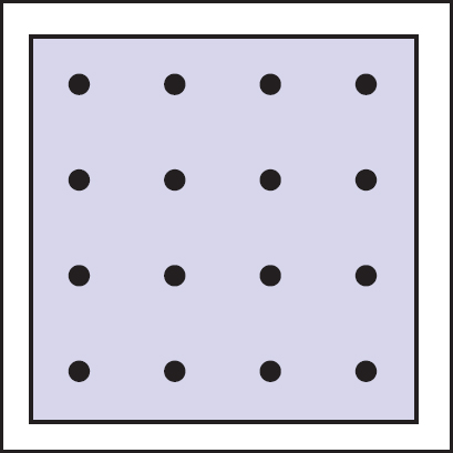
This is usually called regular sampling. The 16 sample locations in a pixel for n = 4 are shown in Figure 13.9. Note that this produces the same answer as rendering a traditional ray-traced image with one sample per pixel at nxn by nyn resolution and then averaging blocks of n by n pixels to get a nx by ny image.
One potential problem with taking samples in a regular pattern within a pixel is that regular artifacts such as moiré patterns can arise. These artifacts can be turned into noise by taking samples in a random pattern within each pixel as shown in Figure 13.10. This is usually called random sampling and involves just a small change to the code:

for each pixel (i, j) do
c = 0
for p = 1 to n2 do
c = c + ray-color(i + ξ, j + ξ)
cij = c/n2
Here ξ is a call that returns a uniform random number in the range [0, 1). Unfortunately, the noise can be quite objectionable unless many samples are taken. A compromise is to make a hybrid strategy that randomly perturbs a regular grid:
for each pixel (i, j) do
c = 0
for p = 0 to n − 1 do
for q = 0 to n − 1 do
c = c + ray-color(i + (p + ξ)/n, j + (q + ξ)/n)
cij = c/n2
That method is usually called jittering or stratified sampling (Figure 13.11).

Sixteen stratified (jittered) samples for a single pixel shown with and without the bins highlighted. There is exactly one random sample taken within each bin.
13.4.2 Soft Shadows
The reason shadows are hard to handle in standard ray tracing is that lights are infinitesimal points or directions and are thus either visible or invisible. In real life, lights have nonzero area and can thus be partially visible. This idea is shown in 2D in Figure 13.12. The region where the light is entirely invisible is called the umbra. The partially visible region is called the penumbra. There is not a commonly used term for the region not in shadow, but it is sometimes called the anti-umbra.

A soft shadow has a gradual transition from the unshadowed to shadowed region. The transition zone is the “penumbra” denoted by p in the figure.
The key to implementing soft shadows is to somehow account for the light being an area rather than a point. An easy way to do this is to approximate the light with a distributed set of N point lights each with one Nth of the intensity of the base light. This concept is illustrated at the left of Figure 13.13 where nine lights are used. You can do this in a standard ray tracer, and it is a common trick to get soft shadows in an off-the-shelf renderer. There are two potential problems with this technique. First, typically dozens of point lights are needed to achieve visually smooth results, which slows down the program a great deal. The second problem is that the shadows have sharp transitions inside the penumbra.

Left: an area light can be approximated by some number of point lights; four of the nine points are visible to p so it is in the penumbra. Right: a random point on the light is chosen for the shadow ray, and it has some chance of hitting the light or not.
Distribution ray tracing introduces a small change in the shadowing code. Instead of representing the area light at a discrete number of point sources, we represent it as an infinite number and choose one at random for each viewing ray. This amounts to choosing a random point on the light for any surface point being lit as is shown at the right of Figure 13.13.
If the light is a parallelogram specified by a corner point c and two edge vectors a and b (Figure 13.14), then choosing a random point r is straightforward:

The geometry of a parallelogram light specified by a corner point and two edge vectors.
where ξ1 and ξ2 are uniform random numbers in the range [0, 1).
We then send a shadow ray to this point as shown at the right in Figure 13.13. Note that the direction of this ray is not unit length, which may require some modification to your basic ray tracer depending upon its assumptions.
We would really like to jitter points on the light. However, it can be dangerous to implement this without some thought. We would not want to always have the ray in the upper left-hand corner of the pixel generate a shadow ray to the upper left-hand corner of the light. Instead we would like to scramble the samples, such that the pixel samples and the light samples are each themselves jittered, but so that there is no correlation between pixel samples and light samples. A good way to accomplish this is to generate two distinct sets of n2 jittered samples and pass samples into the light source routine:
for each pixel (i, j) do
c = 0
generate N = n2 jittered 2D points and store in array r[]
generate N = n2 jittered 2D points and store in array s[]
shuffle the points in array s[]
for p = 0 to N − 1 do
c = c + ray-color(i + r[p].x(), j + r[p].y(), s[p])
cij = c/N
This shuffle routine eliminates any coherence between arrays r and s. The shadow routine will just use the 2D random point stored in s[p] rather than calling the random number generator. A shuffle routine for an array indexed from 0 to N − 1 is:
for i = N − 1 downto 1 do
choose random integer j between 0 and i inclusive
swap array elements i and j
13.4.3 Depth of Field
The soft focus effects seen in most photos can be simulated by collecting light at a nonzero size “lens” rather than at a point. This is called depth of field. The lens collects light from a cone of directions that has its apex at a distance where everything is in focus (Figure 13.15). We can place the “window” we are sampling on the plane where everything is in focus (rather than at the z = n plane as we did previously) and the lens at the eye. The distance to the plane where everything is in focus we call the focus plane, and the distance to it is set by the user, just as the distance to the focus plane in a real camera is set by the user or range finder.

To be most faithful to a real camera, we should make the lens a disk. However, we will get very similar effects with a square lens (Figure 13.16). So we choose the side-length of the lens and take random samples on it. The origin of the view rays will be these perturbed positions rather than the eye position. Again, a shuffling routine is used to prevent correlation with the pixel sample positions. An example using 25 samples per pixel and a large disk lens is shown in Figure 13.17.


An example of depth of field. The caustic in the shadow of the wine glass is computed using particle tracing as described in Chapter 23.
13.4.4 Glossy Reflection
Some surfaces, such as brushed metal, are somewhere between an ideal mirror and a diffuse surface. Some discernible image is visible in the reflection, but it is blurred. We can simulate this by randomly perturbing ideal specular reflection rays as shown in Figure 13.18.

Only two details need to be worked out: how to choose the vector r′ and what to do when the resulting perturbed ray is below the surface from which the ray is reflected. The latter detail is usually settled by returning a zero color when the ray is below the surface.
To choose r′, we again sample a random square. This square is perpendicular to r and has width a which controls the degree of blur. We can set up the square’s orientation by creating an orthonormal basis with w = r using the techniques in Section 2.4.6. Then, we create a random point in the 2D square with side length a centered at the origin. If we have 2D sample points (ξ, ξ′) ∈ [0, 1]2, then the analogous point on the desired square is
Because the square over which we will perturb is parallel to both the u and v vectors, the ray r′ is just
Note that r′ is not necessarily a unit vector and should be normalized if your code requires that for ray directions.
13.4.5 Motion Blur
We can add a blurred appearance to objects as shown in Figure 13.19. This is called motion blur and is the result of the image being formed over a nonzero span of time. In a real camera, the aperture is open for some time interval during which objects move. We can simulate the open aperture by setting a time variable ranging from T0 to T1. For each viewing ray we choose a random time,
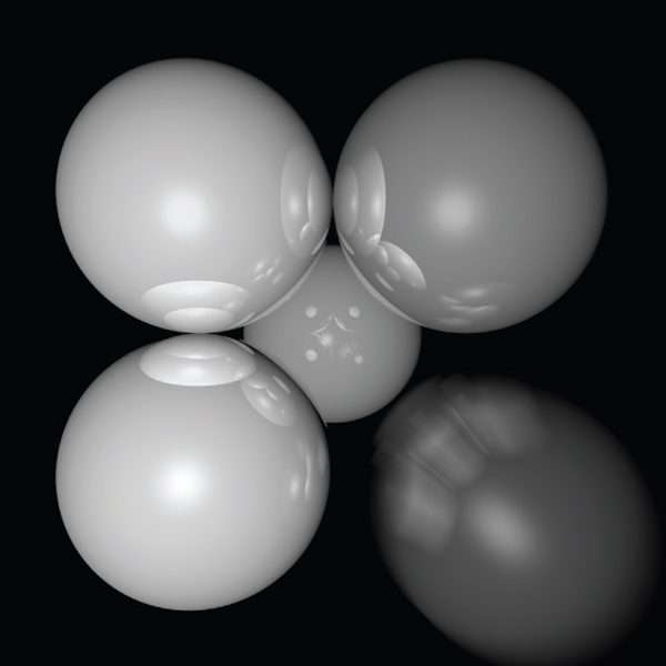
The bottom right sphere is in motion, and a blurred appearance results.
Image courtesy Chad Barb.
We may also need to create some objects to move with time. For example, we might have a moving sphere whose center travels from c0 to c1 during the interval. Given T , we could compute the actual center and do a ray—intersection with that sphere. Because each ray is sent at a different time, each will encounter the sphere at a different position, and the final appearance will be blurred. Note that the bounding box for the moving sphere should bound its entire path so an efficiency structure can be built for the whole time interval (Glassner, 1988).
Notes
There are many, many other advanced methods that can be implemented in the ray-tracing framework. Some resources for further information are Glassner’s An Introduction to Ray Tracing and Principles of Digital Image Synthesis, Shirley’s Realistic Ray Tracing, and Pharr and Humphreys’s Physically Based Rendering: From Theory to Implementation.
Frequently Asked Questions
- What is the best ray-intersection efficiency structure?
The most popular structures are binary space partitioning trees (BSP trees), uniform subdivision grids, and bounding volume hierarchies. Most people who use BSP trees make the splitting planes axis-aligned, and such trees are usually called k-d trees. There is no clear-cut answer for which is best, but all are much, much better than brute-force search in practice. If I were to implement only one, it would be the bounding volume hierarchy because of its simplicity and robustness.
- Why do people use bounding boxes rather than spheres or ellipsoids?
Sometimes spheres or ellipsoids are better. However, many models have polygonal elements that are tightly bounded by boxes, but they would be difficult to tightly bind with an ellipsoid.