
Chapter 22
Implicit Modeling
Brian Wyvill
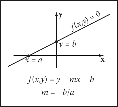
Implicit modeling (also known as implicit surfaces) in computer graphics covers many different methods for defining models. These include skeletal implicit modeling, offset surfaces, level sets, variational surfaces, and algebraic surfaces. In this chapter, we briefly touch on these methods and describe how to build skeletal implicit models in more detail. Curves can be defined by implicit equations of the form
f(x,y)=0.
If we consider a closed curve, such as a circle, with radius r, then the implicit equation can be written as
f(x,y)=x2+y2−r2=0. (22.1)
The value of f(x, y) can be positive (outside the circle), negative (inside the circle), or zero for points precisely on the circle. The equivalent in three dimensions is a closed surface around a set of points that occupy a given volume or region of space. The volume forms a scalar field, i.e., we can compute a value for every point and as can be seen for the circle, the negative values are bounded by the implicit curve or surface. The surface can be visualized as a contour in the field, connecting points with a particular value such as zero (see Equation (22.1)). To compute such a surface implies searching through space to find the points that satisfy the implicit equation; this method is unlikely to lead to an efficient algorithm for circle drawing (and even less likely in three dimensions). This was perhaps the reason that algorithmic methods for modeling with parametric curves and surfaces were investigated before implicit methods; however, there are some good reasons to develop algorithms to visualize implicit surfaces. In this chapter we explore the implications of deriving the data from a modeling process rather than from a scanner.
Despite the computational overhead of finding the implicit surface, designing with implicit modeling techniques offers some advantages over other modeling methods. Many geometric operations are simplified using implicit methods including:
- the definition of blends;
- the standard set operations (union, intersection, difference, etc.) of constructive solid geometry (CSG);
- functional composition with other implicit functions (e.g., R-functions, Barthe blends, Ricci blends, and warping);
- inside/outside tests, (e.g., for collision detection).
Visualizing the surfaces can be done either by direct ray tracing using an algorithm as described in (Kalra & Barr, 1989; Mitchell, 1990; Hart & Baker, 1996; deGroot & Wyvill, 2005) or by first converting to polygons (Wyvill, McPheeters, & Wyvill, 1986).
One of the first methods was proposed by Ricci as far back as 1973 (Ricci, 1973), who also introduced CSG in the same paper. Jim Blinn’s algorithm for finding contours in electron density fields, known as Blobby molecules (J. Blinn, 1982), Nishimura’s Metaballs (Nishimura et al., 1985) and Wyvills’ Soft Objects (Wyvill et al., 1986) were all early examples of implicit modeling methods. Jim Blinn’s Blobby Man (see Figure 22.1) was the first rendering of a non-algebraic implicit model.

22.1 Implicit Functions, Skeletal Primitives, and Summation Blending
In the context of modeling an implicit function is defined as a function f applied to a point p ∈ E3 yielding a scalar value ∈ ℝ.
The implicit function fi(x,y,z) may be split into a distance function di(x,y,z) and a fall-off filter function1 gi(r), where r stands for the distance from the skeleton and the subscript refers to the ith skeletal element.
We will use the following notation:
fi(x,y,z)=gi ∘ di(x,y,z) (22.2)
A simple example is a point primitive, and we take the analogy of a star radiating heat into space. The field value (temperature in this example) may be measured at any point p and can be found by taking the distance from p to the center of the star and supplying the value to a fall-off filter function similar to one of those given in Figure 22.2. In these sample functions, the field is given a value of 1 at the center of the star; the value falls off with distance. The surface of a model may be derived from the implicit function f(x, y, z) as the points of space whose values are equal to some desired iso-value (iso); in the star example, a spherical shell for values of iso ∈ (0, 1).

Fall-off filter functions (0 ≤ r ≤ 1). (a) Blinn’s Gaussian or “Blobby” function; (b) Nishimura’s “Metaball” function; (c) Wyvill et al.’s “soft objects” function; (d) the Wyvill function.
In general, filter functions (gi) are chosen so that the field values are maximized on the skeleton and fall off to zero at some chosen distance from the skeleton. In the simple case where the resulting surfaces are blended together, the global field f(x, y, z) of an object, the implicit function, may be defined as
f(x,y,z)=i=n∑i=1fi(x,y,z), (22.3)
where n skeletal elements contribute to the resulting field value. An example is shown in Figure 22.3 in which the field at any point (x, y, z) is calculated as in Equation (22.3).

Each column shows two point primitives approaching each other. From left to right: the fall-off filter functions used are Blobby, Metaball, soft objects, and Wyvill. Image courtesy Erwin DeGroot.
In this case, two point primitives are placed in close proximity. As the two points are brought together, the surfaces bulge and then blend together. The term filter function is used because the function causes the primitives to be blurred together somewhat akin to a filter function for images. The summation blend is the most compact and efficient blending operation that can be applied to implicit surfaces (see Equation (22.3)).
One advantage of using filter functions with finite support is that primitives that are far from p will have zero contribution and thus need not be considered (Wyvill et al., 1986).
22.1.1 C1 Continuity and the Gradient
The most basic form of continuity is C0 continuity, which ensures that there are no “jumps” in a function. Higher-order continuity is defined in terms of derivatives of functions (see Chapter 15).
In the case of a 3D scalar field f, the first derivative is a vector function known as the gradient, written ∇ f and defined as
∇f(p)={δf(p)δx,δf(p)δy,δf(p)δz}.
If ∇ f is defined at all points, and the three one-dimensional partial derivatives are each C0, then f is C1. Informally, C1 surface continuity means that the surface normal varies smoothly over the surface. The surface normal is the unit vector perpendicular to the surface. If no unique surface normal can be defined on the edge of a cube, for example, then the surface is not C1. For points on an implicit surface, the surface normal can be computed by normalizing the gradient vector ∇f. In the example of the circle, points inside have a negative value and those on the outside have a positive one. For many types of implicit surfaces, the sense of inside and outside is inverted, and since the normal vector must always point outward, it can be opposite to the gradient direction.
Skeletal implicit primitives are created by applying a fall-off filter function to an unsigned distance field as in Equation (22.2). Although the distance field is never C1 at the skeleton, these discontinuities can be removed by using a suitable fall-off function (Akleman & Chen, 1999). If an operator, g, combines implicit functions, f1 and f2, where all points are C1, then g(f1, f2) is not necessarily C1. For example, it is possible to make a sharp CSG junction using the min and max operators. The combination is not C1 continuous because the min and max operators don’t have that property (see Section 22.5).
The analysis of operators is complicated by the fact that it is sometimes desirable to create a C1 discontinuity. This case occurs whenever a crease in the surface is desired. For example, a cube is not C1 because tangent discontinuities occur at each edge. To create creases using C1 primitives, the operator must introduce C1 discontinuities, and hence cannot be C1 itself.
22.1.2 Distance Fields, R-Functions, and F-Reps
The distance field is defined with respect to some geometric object Τ:
F(T,p)=min q∈T|q−p|.
Visually, F(Τ, p) is the shortest distance from p to Τ. Hence, when p lies on Τ, F(Τ, p) = 0 and the surface created by the implicit function is the object Τ. Outside of Τ, a nonzero distance is returned. The function Τ can be any geometric entity embedded in 3D—a point, curve, surface, or solid. Procedural modeling with distance fields started with Ricci (Ricci, 1973); R-functions (Rvachev, 1963) were first applied to shape modeling more than 20 years later (see (Shapiro, 1994) and (A. Pasko, Adzhiev, Sourin, & Savchenko, 1995)).
An R-function or Rvachev function is a function whose sign can change if and only if the sign of one of its arguments changes; that is, its sign is determined solely by its arguments. R-functions provide a robust theoretical framework for Boolean composition of real functions, permitting the construction of Cn CSG operators (Shapiro, 1988). These CSG operators can be used to create blending operators simply by adding a fixed offset to the result (A. Pasko et al., 1995). Although these blending functions are no longer technically R-functions, they have most of the desirable properties and can be mixed freely with R-functions to create complex hierarchical models (Shapiro, 1988). These R-function-based blending and CSG operators are referred to as R-operators (see Section 22.4). The Hyperfun system (Adzhiev et al., 1999) is based on F-reps (function representation), another name for an implicit surface. The system uses a procedural C-like language to describe many types of implicit surfaces.
22.1.3 Level Sets
It is useful to represent an implicit field discretely via a regular grid (Barthe, Mora, Dodgson, & Sabin, 2002) or an adaptive grid (Frisken, Perry, Rockwood, & Jones, 2000). This is exactly what the polygonization algorithm does in the case of level sets; moreover, the grid can be used for various other purposes besides building polygons. Discrete representations of f are commonly obtained by sampling a continuous function at regular intervals. For example, the sampled function may be defined by other volume model representations (V. V. Savchenko, Pasko, Sourin, & Kunii, 1998). The data may also be a physical object sampled using three-dimensional imaging techniques. Discrete volume data has most often been used in conjunction with the level sets method (Osher & Sethian, 1988), which defines a means for dynamically modifying the data structure using curvature-dependent speed functions. Interactive modeling environments based on level sets have been defined (Museth, Breen, Whitaker, & Barr, 2002), although level sets are only one method employing a discrete representation of the implicit field. Methods for interactively defining discrete representations using standard implicit surfaces techniques have also been explored (Baerentzen & Christensen, 2002).
A key advantage to employing a discrete data structure is its ability to act as a unifying approach for all of the various volume models defined by potential fields (discrete or not) (V. V. Savchenko et al., 1998). The conversion of any continuous function to a discrete representation introduces the problem of how to reconstruct a continuous function, needed for the combined purposes of additional modeling operations and visualization of the resulting potential field. A well-known solution to this problem is to apply a filter g using the convolution operator (see Chapter 9). The choice of a filter is guided by the desired properties of the reconstruction, and many filters have been explored (Marschner & Lobb, 1994). The salient point is that there is typically a tradeoff between the efficiency of the chosen filter and the smoothness of the resulting reconstruction; see also Section 22.9.
To be interactive, a discrete system must restrict the size of the grid relative to the available computing power. This, in turn, limits the ability of the modeler to include high-frequency details. Additionally, the smoothing triquadratic filter makes it impossible to include sharp edges, should they be desired. A partial solution to this problem is the use of adaptive grids, although with any discrete representation there will be limitations. A discrete grid is used in (Schmidt, Wyvill, & Galin, 2005) to act as a cache representing a BlobTree node. The grid in this work is used for fast prototyping and uses trilinear interpolation for position and the slower, more accurate triquadratic interpolation to calculate gradient values, because the eye is more discerning in observing gradient errors than position errors.
22.1.4 Variational Implicit Surfaces
It is often required to convert sampled data to an implicit representation. Variational implicit surfaces interpolate or approximate a set of points using a weighted sum of globally supported basis functions (V. Savchenko, Pasko, Okunev, & Kunii, 1995; Turk & O’Brien, 1999; Carr et al., 2001; Turk & O’Brien, 2002). These radially symmetric basis functions are applied at each sample point. The continuity of such a surface depends on the choice of basis function. The C2 thin-plate spline is most commonly used (Turk & O’Brien, 2002; Carr et al., 2001). Like Blinn’s exponential function (see Figure 22.2), this function is unbounded as is the resulting variational implicit surface.
If the field is is globally C2, creases cannot be defined;2 however, anisotropic basis functions can be used to produce fields which change more rapidly and may appear to have creases (Dinh, Slabaugh, & Turk, 2001). At the appropriate scale, the surface is still smooth. The smooth field implies that self-intersections do not occur, and hence volumes are always well-defined. The thin-plate spline guarantees that global curvature is minimized (Duchon, 1977). Variational interpolation has many properties which are desirable for 3D modeling; however, controlling the resulting surfaces can be difficult.
Variational implicit surfaces can also be based on compactly supported radial basis functions (CS-RBFs) to reduce the computational cost of variational interpolation techniques (Morse, Yoo, Rheingans, Chen, & Subramanian, 2001). Each CS-RBF only influences a local region, so computing f(p) requires only evaluation of basis functions within some small neighborhood of p. As with the globally supported counterpart, the resulting field is Ck, creases are not supported, and self-intersections cannot occur.3 The local support of each basis function results in a bounded global field. This also guarantees that additional iso-contours will be present, as noted by various researchers (Ohtake, Belyaev, & Pasko, 2003; Reuter, 2003).
22.1.5 Convolution Surfaces
Convolution surfaces, introduced by Bloomenthal and Shoemake (Bloomenthal & Shoemake, 1991) are produced by convolving a geometric skeleton S with a kernel function h. Hence, the value at any position in space is defined by an integral over the skeleton:
f(p)=∫Sg(r)h(p−r)dr.
Any finitely supported function can be used as h; see (Sherstyuk, 1999) for a detailed analysis of different kernels.
Like skeletal primitives, convolution surfaces have bounded fields. Blinn’s “Blobby molecules” is the simplest form of a convolution surface (J. Blinn, 1982); in this case, the skeleton consists of points only. This idea was extended by Bloomenthal to include line, arc, triangle, and polygon skeletons (Bloomenthal & Shoemake, 1991). These represent 1D and 2D primitives; 3D primitives were later described by Bloomenthal (Bloomenthal, 1995).
Combination of convolution surfaces is defined by composition of the underlying geometric skeletons and has the advantage of eliminating the bulges that tend to occur when composing multiple skeletal primitives with additive blending. The surface resulting from convolution of the combined skeleton does not have bulges, as in Figure 22.4, and the field is continuous even if the combined skeleton is nonconvex. Convolution surfaces are offset a fixed distance from convex portions of a skeleton, but produce a fillet along concave portions of a skeleton.

Two blended cylinders. Left: summation blend; right: convolution surface with barely discernible bulge (Bloomenthal, 1997). Image courtesy Erwin DeGroot.
An example of skeletal elements convolved to build a complex model is shown in Figure 22.5. The hand model contains fourteen primitives.
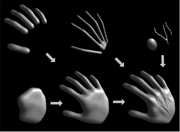
22.1.6 Defining Skeletal Primitives
As we will see in the following sections rendering the implicit models requires finding the field value and gradient for a large number of points. We need the distance to supply to Equation (22.2) and the gradient is useful for root finding as well as lighting calculations. Supplying the distance to the fall-off filter functions of Figure 22.2 is a matter of calculating the nearest distance to the skeletal primitive, simple for point primitives but a little trickier for more complex geometrical shapes. A line segment primitive (AB) can be defined as a cylinder around a line with hemispherical end caps (see Figure 22.6). Point P0 lies on the surface where f(P0) = iso and f(P1) = 0 since it lies outside of the influence of the line primitive. The distance from some Pi to the line is found by simply projecting onto the line AB and calculating the perpendicular distance, e.g., |CP0|; this can be found from AC, since A, P0, and B, are all known:
A→C=A→BA→P0⋅A→B||AB||2.
In Figure 22.6, the field value of P2 > 0, since P2 is in the hemispherical end-cap, which can be checked separately. Variations of this idea can define primitives with endcaps of different radii producing interesting cone shapes. An example is shown in Figure 22.7.

A great variety of geometrical skeletons have been described, and, in principle, it is simply a matter of defining the distance to the skeleton from some point p and also the gradient at p. For example, an offset surface of a triangle can be defined from the vertices of the triangle and a radius r. A simple way to implement this is to use line segment primitives to describe bounding cylinders connecting the vertices (radius r). The distance from a point q within the triangle that does not fall within the bounding fields of one of the line segment primitives is returned as the perpendicular distance to the plane of the triangle. Other examples include an implicit disk, defined by a circle and a thickness parameter, a torus also defined by a circle and the radius of the cross section (or inner and outer circle radii), a circular cone from a disk and a height, a cube with rounded corners, etc. (see Figure 22.8).


A ray-traced dinosaur model showing the underlying skeletal primitives. Image courtesy Erwin DeGroot.
22.2 Rendering
Modeling methods, such as parametric surfaces, lend themselves to visualization, since it is easy to iterate over points on the surface that can be found directly from the defining equations; for example (x, y) = (cos θ, sin θ), θ ∈ [0, 2π) produces a circle.
There are two techniques that are commonly used to render implicit surfaces: ray tracing and surface tiling. In practice, a designer wants to visualize an implicit surface model quickly, sacrificing quality for speed for interaction purposes. Prototyping algorithms have been concerned with producing a polygon mesh that can be rendered in real time on modern workstations. Finding the polygonal mesh which best approximates the desired surface is referred to as polygonization or surface tiling. For animation or for a final visualization, where quality is preferred over speed, ray tracing implicit surfaces directly without first polygonizing produces excellent results.
As previously mentioned, finding an implicit surface requires searching through space to find the points that satisfy, f(p) = 0. There are two main approaches to executing such a search: space partitioning—partitioning space into manageable units such as cubes, and non-space partitioning, e.g., marching triangles (Hartmann, 1998; Akkouche & Galin, 2001) and the shrinkwrap algorithm (van Overveld & Wyvill, 2004).
In this chapter, we describe the original space partitioning algorithm and leave it to the reader to explore the more advanced methods. This algorithm together with postprocessing for mesh refinement (see Chapter 12) and caching provide a method for interactive viewing of implicit models on modern workstations.
22.3 Space Partitioning
22.3.1 Exhaustive Search
The basic cubic space partitioning algorithm for tiling implicit surfaces was first published in (Wyvill et al., 1986) and a similar algorithm oriented toward volume visualization, called marching cubes in (Lorensen & Cline, 1987). Since then there have been many refinements and extensions.
A first approach to finding the implicit surface might be to subdivide space uniformly into a regular lattice of cubic cells and calculate a value for every vertex. Each cell is replaced with a set of polygons that best approximates the part of the surface contained within that cell. The problem with this method is that many of the cells will be completely outside or completely inside the volume; thus, many cells that contain no part of the surface are processed. For large grids of data this can be very time consuming and memory intensive.
To avoid storing the whole grid, a hash table is used to store only the cubes that contain a piece of the surface, based on the data structures used in (Wyvill et al., 1986). Working software was published in Graphics Gems IV (Bloomenthal, 1990). The algorithm is based on numerical continuation; it starts with a seed cube that intersects part of the surface and builds neighboring cubes as necessary to follow the surface.
The algorithm has two parts. In the first part, cubic cells are found that contain the surface and in the second part, each cube is replaced by triangles. The first part of the algorithm is driven by a queue of cubes, each of which contains part of the surface; the second part of the algorithm is table-driven.
22.3.2 Algorithm Description
A fast overview of the algorithm is as follows:
- divide space into cubic voxels;
- search for surface, starting from a skeletal element;
- add voxel to queue, mark it visited;
- search neighbors;
- when done, replace voxel with polygons.
First, space is subdivided into a cubic lattice, and the next task is to find a seed cube containing part of the surface. A cube vertex vi inside the surface will have a field value vi > = iso and a vertex outside the surface will have a field value vi < iso; thus, an edge with one of each type of vertex will intersect the surface. We call this an intersecting edge. The field value at the nearest cube vertex to the first primitive can be evaluated by summing the contributions of the primitives as per Equation (22.3), although other operators can also be used as will be seen later. We will assume that f(v0) > iso, which indicates that v0 lies within the solid. The value of iso is chosen by the user; an example is iso = 0.5 when using the soft fall-off function, which has some symmetry properties that lead to nice blending (see Figure 22.3). The vertices along one axis are evaluated in turn until a value vi < iso is found. The cube containing the intersecting edge is the seed cube.
The neighbors of the seed cube are examined, and those that contain at least one intersecting edge are added to the queue ready for processing. To process a cube, we examine each face. If any of the bounding edges have oppositely signed vertices, the surface will pass through that face and the face neighbor must be processed. When this process has been completed for all the faces, the second phase of the algorithm is applied to the cube. If the surface is closed, eventually a cube will be revisited and no more unmarked neighbors found, and the search algorithm will terminate. Processing a cube involves marking it as processed and processing its unmarked neighbors. Those that contain intersecting edges are processed until the entire surface has been covered (see Figure 22.10).

A section through the cubic lattice. The + sign indicates a vertex inside the surface (f(vi ≥ iso) and - is outside f(vi < iso).
Each cube is indexed by an identifying vertex which we define to be the lower-leftfar corner (i.e., the vertex with the lowest (x, y, z)-coordinate values (see Figure 22.11)). For each vertex that is inside the surface, the corresponding bit will be set to form the address in an 8-bit table (see Figure 22.11 and Section 22.3.3).
The identifying vertex is addressed by integers i, j, k, computed from the (x, y, z)-coordinate location of the cube such that x = side * i, etc., where side is the size of the cube. The identifying vertex of each cube may appear in as many as eight other cubes, and it would be inefficient to store these vertices more than once. Thus, the vertices are stored uniquely in a chained hash table. Since most of the space does not contain any part of the surface, only those cubes that are visited will be stored. The implicit function value is found for each vertex as it is stored in the hash table.
Nothing is known about the topology of the surface so a search must be started from every primitive to avoid any disconnected parts of the surface being missed. A scalar can be used to scale the influence of a primitive. If the scalar can be less than zero, then it is possible to search along an axis without finding an intersecting edge. In this case, a more sophisticated search must be done to find a seed cube (Galin & Akkouche, 1999).
Data Structures
The hash table entry holds five values:
- the i, j, k lattice indices of the identifying vertex (see Figure 22.11);
- f, the implicit function value of the identifying vertex;
- Boolean to indicate whether this cube has been visited.

The hash function computes an address in the hash table by selecting a few bits out of each of i, j, k and combining them arithmetically. For example, the five least significant bits produces a 15-bit address for a table, which must have a length of 215. Such a hash function can be neatly implemented in the C-preprocessor as follows:
#define NBITS 5
#define BMASK 037
#define HASH(a,b,c) (((a&BMASK)≪NBITS|b&BMASK) ≪NBITS|c&BMASK)
#define HSIZE 1≪NBITS*3
The queue (FIFO list) is used as temporary storage to identify the neighbors for processing. The algorithm begins with a seed cube that is marked as visited and placed on the queue. The first cube on the queue is dequeued and all its unvisited neighbors are added to the queue. Each cube is processed and passed to the second phase of the algorithm if it contains part of the surface. The queue is then processed until empty.
22.3.3 Polygonization Algorithm
The second phase of the algorithm treats each cube independently. The cell is replaced by a set of triangles that best matches the shape of the part of the surface that passes through the cell. The algorithm must decide how to polygonize the cell given the implicit function values at each vertex. These values will be positive or negative (i.e., less than or greater than the iso-value), giving 256 combinations of positive or negative vertices for the eight vertices of the cube. A table of 256 entries provides the right vertices to use in each triangle (Figure 22.12). For example, entry 4(00000100) points to a second table that records the vertices that bound the intersecting edges. In this example, vertex number 2 is inside the surface (f(V2) > = iso) and, therefore, we wish to draw a triangle that connects the points on the surface that intersect with edges bounded by (V2, V0), (V2, V3), and (V2, V6) as shown in Figure 22.13.

Table 2 contains the edges intersected by the surface. Table 1 points to the appropriate entry in Table 2.

Finding Cube-Surface Intersections
Figure 22.13 shows a cube where vertex V2 is inside the surface and all other vertices are outside. Intersections with the surface occur on three edges as shown. The surface intersects edge V2 – V6 at the point A. The fastest, but inaccurate, way to calculate A is to use linear interpolation:
f(A)−f(V2)f(V6)−f(V2)=|A−V2|side.
If the cube side is 1 and the iso-value sought for f(A) is 0.5, then
A=V3+0.5−f(V2)f(V6)−f(V2).
This works well for a static image, but in animation error differences between frames will be very noticeable. A root-finding method such as regula falsi should be employed. This becomes more computationally costly as the gradient is needed to evaluate the point of intersection. The gradient is also needed at surface points for rendering. For many types of primitives it is simpler to find a numerical approximation using sample points around p, as in
∇f(p)=(f(p+Δx)−f(p)Δx,f(p+Δy)−f(p)Δy,f(p+Δz)−f(p)Δz).
A reasonable value for Δ has been found empirically to be 0.01 * side where side is the length of a cube edge.
For manufacturing a mesh, as opposed to a set of independent triangles, a second hash table can maintain a list of all the intersecting edges. Since each cube edge is shared by up to four neighbors, the edge hash table prevents repetition of the surface-cube edge intersection calculation. The hash address can be derived from the same hash function as for vertices (applied to the edge endpoints).
22.3.4 Sampling Problems
Ambiguities occur when opposite corners of a face (or the cube) have the same sign and the other pair of vertices on the face have the opposite sign (see Figure 22.14). A sample taken in the center of the face will give a clue as to whether the cube represents the meeting of two surfaces or a saddle. It should be made clear that a spatial grid stores a sample of the implicit function at every vertex. If the function happens to vary considerably within a cell, the polygonal representation will not show such variations (see Figure 22.15). The surface cannot be resolved by sampling alone unless something is known about the curvature of the surface. A good discussion of this topic appears in (Kalra & Barr, 1989).

Examples of vertices inside (+) and outside (-) the surface. Note the extra sample gives a clue to avoid ambiguous cases.

This ambiguity problem (not the undersampling problem) is avoided by subdividing the cubic cell into tetrahedra. The tetrahedra can then be polygonized unambiguously. Since there are four vertices in each tetrahedron, a table of 16 entries will provide the correct triangle information. The disadvantage is that approximately twice the number of polygons will be generated.
Subdividing a Cube
Without requiring additional cell vertices, a cube may be decomposed into five or six tetrahedra as shown in Figure 22.16. These decompositions introduce diagonals on the cube faces, and to maintain a consistent diagonal direction between neighbors, the six decomposition is preferable. The introduction of diagonal edges produces a higher-resolution surface than replacing each cube directly with triangles. The decomposition into tetrahedra and the replacement of the tetrahedra with triangles are fast, table-driven algorithms, which produce topologically consistent meshes.

22.3.5 Cell Polygonization
Two obvious problems emerge from the use of uniform space subdivision. The size of triangles output by this algorithm do not adapt to the curvature of the surface and a further sample is required to solve the ambiguities, in which cubic cells are replaced by polygons. A space subdivision algorithm based on an octree was developed by Bloomenthal (Bloomenthal, 1988), which does adapt to the curvature of the surface. Cells are subdivided into eight octants and cracks are avoided by using a restricted octree scheme, i.e., neighboring cells cannot differ by more than one level of subdivision. This indeed reduces the number of polygons generated, but full advantage of large cells can only be taken if the flat regions of the surface happen to fall entirely within the appropriate octants. The algorithm proves in practice to be considerably slower than the uniform voxel algorithm and is more complicated to implement.
22.4 More on Blending
Section 22.1 showed that blending can be made to occur when field values are summed. Ricci, in his landmark paper (Ricci, 1973), describes super-elliptic blending. Given two functions FA and FB, previously we simply found the implicit value as Ftotal = FA + FB. We can denote this more general blending operator as A ◊ B. The Ricci blend is defined as:
fA⋄B=(fAn+fBn)1n. (22.4)
It is interesting to point out the following properties:
lim n→+∞(fAn+fBn)1n=max(fA,fB),lim n→+∞(fAn+fBn)1n=min (fA,fB).
Moreover, this generalized blending is associative, i.e., f(A◊B)◊C = fA◊(B◊C). The standard blending operator + proves to be a special case of the super-elliptic blend with n = 1. When n varies from 1 to infinity, it creates a set of blends interpolating between blending A + B and union A ∪ B (see Figure 22.17). Figure 22.27 shows the nodes to be binary or unary; in fact the binary nodes can easily be extended using the above formulation to n-ary nodes.

By varying n, the Ricci blend may be made to change smoothly from blend to union. Image courtesy Erwin DeGroot.
The power of Ricci’s operators is that they are closed under the operations on the space of all possible implicit volumes, meaning that an application of an operator simply produces another scalar field defining another implicit volume. This new field can be composed with other fields, again using Ricci’s operators. Equation (22.4) will always produce the exact union of two implicit volumes, regardless of how complex they are. Compared with the difficulties involved in applying Boolean CSG operations to B-rep surfaces, solid modeling with implicit volumes is incredibly simple.
Following Pasko’s functional representation (A. Pasko et al., 1995), another generalized blending function may be defined:
fA⋄B=(fA+fB+α√fA2+fB2)(fA2+fB2)n2.
When α ∈ [−1, 1] varies from −1 to 1, it creates a set of blends interpolating the union and the intersection operators. However, this operator is no longer associative which is incompatible with the definition of n-ary operators.
22.5 Constructive Solid Geometry
Implicit models are frequently termed implicit surfaces; however, they are inherently volume models and useful for solid modeling operations. Ricci introduced a constructive geometry for defining complex shapes from operations such as union, intersection, difference, and blend upon primitives (Ricci, 1973). The surface was considered as the boundary between the half spaces f(p) < 1, defining the inside, and f(p) > 1 defining the outside. This initial approach to solid modeling evolved into constructive solid geometry or CSG (Ricci, 1973; Requicha, 1980). CSG is typically evaluated bottom-up according to a binary tree, with low-degree polynomial primitives as the leaf nodes and internal nodes representing Boolean set operations. These methods are readily adapted for use in implicit modeling, and in the case of skeletal implicit surfaces, the Boolean set operations union ∪max, intersection ∩min and difference minmax are defined as follows (Wyvill, Galin, & Guy, 1999):
∪max f=k−1max i=0(fi),∩min f=k−1min i=0(fi),minmax f=min(f0,2*iso−k−1max j=1(fj)). (22.5)
The Ricci operators are illustrated in Figure 22.18 for point primitives A and B. For union (bottom left) the field at all points inside the union will be the greater of fA() and fB(). For intersection (center), points in the region marked as P1 will have value min (fA(P1), fB (P1)) = 0, since the contribution of B will be zero outside of its range of influence. Similarly, for the region marked as P2, (influence of A is zero, i.e., the minimum) leaving only the intersection region with positive values. Difference works similarly using the iso-value in the three marked regions (Pi) as follows:
f(P0)=min (fB(P0),2*iso−fA(P0))=min ([iso, 1],[2*iso−1,iso])=[2*iso−1, iso]<isof(P1)=min (fB(P1),2*iso−fA(P1))=min ([0, iso],[2*iso−1,iso])<isof(P2)=min (fB(P2),2*iso−fA(P2))=min ([iso, 1],[iso, 2*iso])>=iso

CSG operators create creases, i.e., C1 discontinuities. For example, the min() operator (Equation (22.5)) creates C1 discontinuities at all points where f1(p) = f2(p). When applied to two spheres, the discontinuities produced by this union operator result in a crease on the surface, as shown in Figure 22.18, which is the desired result. Discontinuities unfortunately extend into the field outside of the surface, which is not visible in this image. If a blend is then applied to the result of the union, the C1-discontinuous plane in the field produces a shading discontinuity (Figure 22.19).

Two point primitives on the left are connected by the Ricci union. A third primitive is blended to the result, creating an unwanted crease in the field. Image courtesy Erwin DeGroot.
The problem can be avoided to an extent (G. Pasko, Pasko, Ikeda, & Kunii, 2002), and CSG operators have been developed that are C1 at all points except those where f1(p) = f2(p) = iso (Barthe, Dodgson, Sabin, Wyvill, & Gaildrat, 2003).
22.6 Warping
The ability to distort the shape of a surface by warping the space in its neighborhood is a useful modeling tool. A warp is a continuous function w(x, y, z) that maps ℝ3 onto ℝ3. Sederberg provides a good analogy for warping when describing free form deformations (Sederberg & Parry, 1986). He suggests that the warped space can be likened to a clear, flexible, plastic parallelepiped in which the objects to be warped are embedded. A warped element may be defined by simply applying some warp function w(p) to the implicit equation:
fi(x,y,z)=gi∘di∘wi(x,y,z). (22.6)
A warped element may be fully characterized by the distance to its skeleton di(x, y, z), its fall-off filter function gi(r), and eventually its warp function wi(x, y, z). To render or perform operations on an implicit surface, the implicit value of many points f(P) must be found. First, P is transformed by the warp function to some new point Q, and f(Q) is returned in place of f(P). In Figure 22.20, instead of returning the implicit value of some point f(Q), the value for f(P) is returned. In this case, the iso-value is returned and the implicit surface (curve in 2D) passes through Q instead of P. Thus, the circle is warped into an ellipse.

Barr introduced the notion of global and local deformations using the operations of twist, taper, and bend applied to parametric surfaces (Barr, 1984). The deformations can be nested to produce models such as the one shown in Figure 22.27. Conceptually, these are easy to apply to an implicit surface, as indicated in Equation (22.6).
Note that the normal cannot be calculated in a similar manner to warping a point. This problem is similar to the problem outlined in Section 13.2 on instancing. In this case, the normal can most easily be approximated using Equation (22.3.3) although the use of the Jacobian, as suggested in (Barr, 1984), yields precise results. The Barr warps are described in the following sections.
22.6.1 Twist
In this example, the twist is around the z-axis by θ (see Figure 22.21) for three blended implicit cylinders with a twist warp applied to them.

The twist around z is expressed as
w(x,y,z)={x*cos (θ(z))−y*sin (θ(z))x*sin (θ(z))+y*cos (θ(z))z}.
22.6.2 Taper
Taper is applied along one major axis. A linear taper has proved to be the most useful although quadratic and cubic tapers are easily implemented. For example, a linear taper along the y-axis involves changing both x- and z-coordinates. (See Figure 22.22.) A linear scale is applied to y between ymax and ymin:
s(y)=ymax −yymax −ymin w(x,y,z)={s(y)xys(y)z}
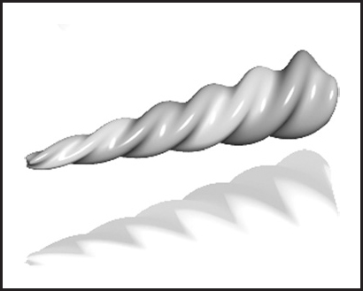
22.6.3 Bend
Bend is also applied along one major axis. (See Figure 22.23.) For the bend example below, the bending rate is k measured in radians per unit length, the axis of the bend is (x0, 1/k), and the angle θ is defined as (x – x0) * k. The bend around z is

Three blended implicit cylinders, twisted together, tapered and bent. Image courtesy Erwin DeGroot.
w(x,y,z)={−sin (θ)*(y−1/k)+x0cos (θ)*(y−1/k)+1/kz}
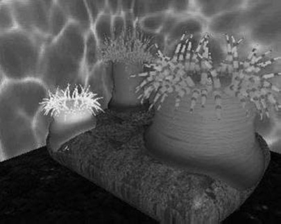
22.7 Precise Contact Modeling
Precise contact modeling (PCM) is a method of deforming implicit surface primitives in contact situations while maintaining a precise contact surface with C1 continuity (Gascuel, 1993). PCM is important in that it is a simple and automatic way of showing how a model can react to its environment. This cannot be so easily done with non-implicit methods (see Figure 22.24).
PCM is implemented by the inclusion of a deforming function s(p) that modifies the field value returned for each point. For each pair of objects, collision is first detected using a bounding-box test. Once it is established that a collision is likely, PCM is applied. A local, geometric deformation term si is computed and added to the implicit function fi. The volume of the colliding objects is divided into an interpenetration region and a deformation region. The result of applying si is that the interpenetration region is compressed so that contact is maintained without interpenetration occurring (see Figure 22.25). The effect of si is attenuated to zero within the propagation region so that the volume outside of the two regions is not deformed.

A 2D slice through objects in collision showing the various regions and PCM deformation. Image courtesy Erwin DeGroot.
Given two skeletal elements generating fields f1(p) and f2(p), the surface around each one is calculated as
f1(p)+s1(p)=0,f2(p)+s2(p)=0.
We need to generate a surface common to both elements (dotted line in Figure 22.25), i.e., where they share a solution in the interpenetration region for some p in that region:
s1(p)−f1(p)=iso,s2(p)−f2(p)=iso. (22.7)
Intuitively, the deeper within object 1 that object 2 penetrates, the higher the implicit value of object 1 and thus the more that object 2 will be compressed.
The function, si is defined to produce a smooth junction at the boundary of the interpenetration region, in other words where si = 0 but its derivative is greater than zero. From here to the boundary of the propagation region, si is used to attenuate the propagation to zero. The nearest point on the interpenetration region boundary po is found by following the gradient.
Within the propagation region si(p) = hi(r), where p = (x, y, z) is the point whose implicit value is being calculated and r = ∥p–po∥ (see Figure 22.26). The value of ri, set by the user, defines the size of the propagation region; no deformation occurs beyond this region. To control how much the objects inflate in the propagation region, the user provides a value for the parameter α. The maximum value of hi is Mi. The current minimum of si is negative in the interpenetration region and is given as simin, where Mi = −αisimin. Thus an object will be compressed in the interpenetration region and will inflate in the propagation region. The equation for hi is formed in two parts by two cubic polynomials that are designed to join at r = ri/2, where the slope is zero:

The function, hi(r) is the value of the deformation function wi in the propagation region.
It is desirable that we have C1-continuity as we move from the interpenetration to the propagation region. Thus, in Figure 22.26, is the directional derivative of si at the junction (marked as p0 in Figure 22.25). As indicated in Equation (22.7), si = −fi in the interpenetration region, thus:
PCM is only an approximation to a properly deformed surface, but it is an attractive algorithm due to its simplicity.
22.8 The BlobTree
The BlobTree is a method that employs a tree structure that extended the CSG tree to include various blending operations using skeletal primitives (Wyvill et al., 1999). A system with similar capabilities, the Hyperfun project, used a specialized language to describe F-rep objects (Adzhiev et al., 1999).
In the BlobTree system, models are defined by expressions that combine implicit primitives and the operators ∪ (union), ∩ (intersection), − (difference), + (blend), ◊ (super-elliptic blend), and w (warp). The BlobTree is not only the data structure built from these expressions but also a way of visualizing the structure of the models. The operators listed above are binary with the exception of warp, which is a unary operator. In general it is more efficient to use n-ary rather than binary operators. The BlobTree incorporates affine transformations as nodes so that it is also a scene graph and primitives (e.g., skeletons) form the leaf nodes.
22.8.1 Traversing the BlobTree
An example of a BlobTree including the Barr warps and CSG operations is shown in Figure 22.27. Other nodes can include 2D texturing (Schmidt, Grimm, & Wyvill, 2006), precise contact modeling, as well as animation and other attributes. The traversal of the BlobTree is in essence very simple. All that is required to render the object either by polygonizing or ray tracing is to find the implicit value of any point (and the corresponding gradient). This can be done by traversing the tree. Polygonization and ray-tracing algorithms need to evaluate the implicit field function at a large number of points in space. The function f(N, M) returns the field value for the node N at the point M, which depends on the type of the node. The values L and R indicate that the left or right branch of the tree is explored. The algorithm below is written (for simplicity) as if the tree were binary:
function f (N, M):
- primitive: f(M);
- warp: f(L(N), w(M));
- blend: f(L(N), M) + f(R(N), M));
- union: max(f(L(N), M), f(R(N), M));
- intersection: min(f(L(N), M), f(R(N), M));
- difference: min(f(L(N), M), −f(R(N), M)).
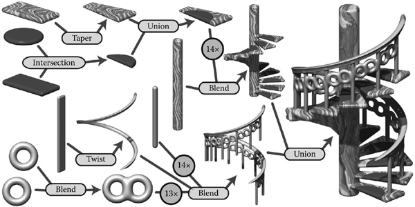
BlobTree. The spiral staircase is built from a central textured cylinder to which the stairs and the railing are blended. The railing is comprised of a series of cylinders blended with two circle (torus) primitives, blended together and further blended with a vertical cylinder. The BlobTree is also a scene graph and instancing nodes repeat the various parts transformed by the appropriate matrices. Each stair is made from a tapered polygon primitive (that becomes an offset surface); intersection and union nodes combine the inflated disk with the stair.
A complex BlobTree model showing many of the features that have been integrated is shown in Figure 22.28.

“Spiral Stairs.” A complex BlobTree implicit model created in Erwin DeGroot’s BlobTree.net system.
22.9 Interactive Implicit Modeling Systems
Early sketch-based modeling systems, such as Teddy (Igarashi, Matsuoka, & Tanaka, 1999), used a few drawn strokes from the user to infer a polygonal model in 3-space. With better hardware and improved algorithms, sketch-based implicit modeling systems are now possible. Shapeshop uses implicit sweep surfaces to manufacture 3D strokes from 2D user strokes and also preserves the hierarchy of the BlobTree unlike the early systems that produced homogeneous meshes (Schmidt, Wyvill, Sousa, & Jorge, 2005). This enables a user to produce complex models of arbitrary topology from a few simple strokes. The margin figures show a closed drawn stroke (Figure 22.29) inflated into a an implicit sweep and a second sweep (Figure 22.30) that has a smaller sweep object subtracted using CSG.


BlobTree operations can be applied, e.g., CSG difference. Image courtesy Erwin DeGroot.
One of the improvements that made this possible is a caching system that uses a fixed 3D grid of implicit values at each node of the BlobTree representing the values found by traversing the tree below the node (Schmidt, Wyvill, & Galin, 2005). If the value of some point p is required at node N, a value may be returned without traversing the tree below N, provided that part of the tree is unaltered. Instead, an interpolation scheme (see Chapter 9) is used to find a value for p. This scheme speeds up traversal for complex BlobTrees and is one factor in enabling a system to run at interactive rates.
The next generation of implicit modeling systems will exploit hardware and software advances to be able to handle more and more complex hierarchical models interactively. A more complex Shapeshop example is shown in Figure 22.31.

“The Next Step.” A complex BlobTree implicit model created interactively in Ryan Schmidt’s Shapeshop by artist Corien Clapwijk (Andusan).
Exercises
In an implicit surface modeling system the fall-off filter function is defined as
where R is a constant. A point primitive placed at (—1,0) and another at (1, 0) are rendered to show the f = 0.5 iso-surface. The value R, the distance where the potential due to the point falls to zero in both cases, is 1.5.
Calculate the potential at the point (0,0) and at +0.5 intervals until the point (2.5, 0). Sketch the 0.5 contour and the contour at which the field falls to zero.
- Why are the ambiguous cases in the polygonization algorithm considered to be a sampling problem?
- Calculate the error involved in using linear interpolation to estimate the intersection of an implicit surface and a cubic voxel.
- Design an implicit primitive function using the skeleton of your choice. The function must take as input a point and return an implicit value and also the gradient at that point.
1These functions have been given many names by researchers in the past, e.g., filter, potential, radial-basis, kernel, but we use fall-off filter as a simple term to describe their appearance.
2Except see Section 15.2.
3Note, k > 0 depending on the RBF (see Section 15.2).