Chapter 8

The Graphics Pipeline

The previous several chapters have established the mathematical scaffolding we need to look at the second major approach to rendering: drawing objects one by one onto the screen, or object-order rendering. Unlike in ray tracing, where we consider each pixel in turn and find the objects that influence its color, we’ll now instead consider each geometric object in turn and find the pixels that it could have an effect on. The process of finding all the pixels in an image that are occupied by a geometric primitive is called rasterization, so object-order rendering can also be called rendering by rasterization. The sequence of operations that is required, starting with objects and ending by updating pixels in the image, is known as the graphics pipeline.

Object-order rendering has enjoyed great success because of its efficiency. For large scenes, management of data access patterns is crucial to performance, and making a single pass over the scene visiting each bit of geometry once has significant advantages over repeatedly searching the scene to retrieve the objects required to shade each pixel.

The title of this chapter suggests that there is only one way to do objectorder rendering. Of course this isn’t true—two quite different examples of graphics pipelines with very different goals are the hardware pipelines used to support interactive rendering via APIs like OpenGL and Direct3D and the software pipelines used in film production, supporting APIs like RenderMan. Hardware pipelines must run fast enough to react in real time for games, visualizations, and user interfaces. Production pipelines must render the highest quality animation and visual effects possible and scale to enormous scenes, but may take much more time to do so. Despite the different design decisions resulting from these divergent goals, a remarkable amount is shared among most, if not all, pipelines, and this chapter attempts to focus on these common fundamentals, erring on the side of following the hardware pipelines more closely.

The work that needs to be done in object-order rendering can be organized into the task of rasterization itself, the operations that are done to geometry before rasterization, and the operations that are done to pixels after rasterization. The most common geometric operation is applying matrix transformations, as discussed in the previous two chapters, to map the points that define the geometry from object space to screen space, so that the input to the rasterizer is expressed in pixel coordinates, or screen space. The most common pixelwise operation is hidden surface removal which arranges for surfaces closer to the viewer to appear in front of surfaces farther from the viewer. Many other operations also can be included at each stage, thereby achieving a wide range of different rendering effects using the same general process.

For the purposes of this chapter, we’ll discuss the graphics pipeline in terms of four stages (Figure 8.1). Geometric objects are fed into the pipeline from an interactive application or from a scene description file, and they are always described by sets of vertices. The vertices are operated on in the vertex-processing stage, then the primitives using those vertices are sent to the rasterization stage. The rasterizer breaks each primitive into a number of fragments, one for each pixel covered by the primitive. The fragments are processed in the fragment processing stage, and then the various fragments corresponding to each pixel are combined in the fragment blending stage.

We’ll begin by discussing rasterization, then illustrate the purpose of the geometric and pixel-wise stages by a series of examples.

8.1 Rasterization

Rasterization is the central operation in object-order graphics, and the rasterizer is central to any graphics pipeline. For each primitive that comes in, the rasterizer has two jobs: it enumerates the pixels that are covered by the primitive and it interpolates values, called attributes, across the primitive—the purpose for these attributes will be clear with later examples. The output of the rasterizer is a set of fragments, one for each pixel covered by the primitive. Each fragment “lives” at a particular pixel and carries its own set of attribute values.

In this chapter, we will present rasterization with a view toward using it to render three-dimensional scenes. The same rasterization methods are used to draw lines and shapes in 2D as well—although it is becoming more and more common to use the 3D graphics system “under the covers” to do all 2D drawing.

8.1.1 Line Drawing

Most graphics packages contain a line drawing command that takes two endpoints in screen coodinates (see Figure 3.10) and draws a line between them. For example, the call for endpoints (1,1) and (3,2) would turn on pixels (1,1) and (3,2) and fill in one pixel between them. For general screen coordinate endpoints (x0, y0) and (x1, y1), the routine should draw some “reasonable” set of pixels that approximates a line between them. Drawing such lines is based on line equations, and we have two types of equations to choose from: implicit and parametric. This section describes the approach using implicit lines.

Line Drawing Using Implicit Line Equations

The most common way to draw lines using implicit equations is the midpoint algorithm (Pitteway (1967); van Aken and Novak (1985)). The midpoint algorithm ends up drawing the same lines as the Bresenham algorithm (Bresenham, 1965) but it is somewhat more straightforward.

The first thing to do is find the implicit equation for the line as discussed in Section 2.5.2:

$f\left(x,y\right)\equiv \left(y_0-y_1\right)x+\left(x_1-x_0\right)y+x_0{y}_1-x_1{y}_0=0.\text{ (8.1)}$

We assume that x0 ≤ x1. If that is not true, we swap the points so that it is true. The slope m of the line is given by

$m=\frac{y_1-y_0}{x_1-x_0}.$

The following discussion assumes m ∈ (0, 1]. Analogous discussions can be derived for m ∈ (−∞, −1], m ∈ (−1, 0], and m ∈ (1, ∞). The four cases cover all possibilities.

For the case m ∈ (0, 1], there is more “run” than “rise,” i.e., the line is moving faster in x than in y. If we have an API where the y-axis points downward, we might have a concern about whether this makes the process harder, but, in fact, we can ignore that detail. We can ignore the geometric notions of “up” and “down,” because the algebra is exactly the same for the two cases. Cautious readers can confirm that the resulting algorithm works for the y-axis downward case. The key assumption of the midpoint algorithm is that we draw the thinnest line possible that has no gaps. A diagonal connection between two pixels is not considered a gap.

As the line progresses from the left endpoint to the right, there are only two possibilities: draw a pixel at the same height as the pixel drawn to its left, or draw a pixel one higher. There will always be exactly one pixel in each column of pixels between the endpoints. Zero would imply a gap, and two would be too thick a line. There may be two pixels in the same row for the case we are considering; the line is more horizontal than vertical so sometimes it will go right, and sometimes up. This concept is shown in Figure 8.2, where three “reasonable” lines are shown, each advancing more in the horizontal direction than in the vertical direction.

The midpoint algorithm for m ∈ (0, 1] first establishes the leftmost pixel and the column number (x-value) of the rightmost pixel and then loops horizontally establishing the row (y-value) of each pixel. The basic form of the algorithm is:

y = y0

for x = x0 to x1 do

 draw(x, y)

 if (some condition) then

 y = y + 1

Note that x and y are integers. In words this says, “keep drawing pixels from left to right and sometimes move upward in the y-direction while doing so.” The key is to establish efficient ways to make the decision in the if statement.

An effective way to make the choice is to look at the midpoint of the line between the two potential pixel centers. More specifically, the pixel just drawn is pixel (x, y) whose center in real screen coordinates is at (x, y). The candidate pixels to be drawn to the right are pixels (x + 1, y) and (x + 1, y + 1). The midpoint between the centers of the two candidate pixels is (x + 1, y + 0.5). If the line passes below this midpoint we draw the bottom pixel, and otherwise we draw the top pixel (Figure 8.3).

To decide whether the line passes above or below (x + 1, y + 0.5), we evaluate f(x, y + 0.5) in Equation (8.1). Recall from Section 2.5.1 that f(x, y) = 0 for points (x, y) on the line, f(x, y) > 0 for points on one side of the line, and f(x, y) < 0 for points on the other side of the line. Because −f(x, y) = 0 and f(x, y) = 0 are both perfectly good equations for the line, it is not immediately clear whether f(x, y) being positive indicates that (x, y) is above the line, or whether it is below. However, we can figure it out; the key term in Equation (8.1) is the y term (x1 – x0)y. Note that (x1 – x0) is definitely positive because x1 > x0. This means that as y increases, the term (x1–x0)y gets larger (i.e., more positive or less negative). Thus, the case f(x, +∞) is definitely positive, and definitely above the line, implying points above the line are all positive. Another way to look at it is that the y component of the gradient vector is positive. So above the line, where y can increase arbitrarily, f(x, y) must be positive. This means we can make our code more specific by filling in the if statement:

if f(x + 1, y + 0.5) < 0 then

  y = y + 1

The above code will work nicely for lines of the appropriate slope (i.e., between zero and one). The reader can work out the other three cases which differ only in small details.

If greater efficiency is desired, using an incremental method can help. An incremental method tries to make a loop more efficient by reusing computation from the previous step. In the midpoint algorithm as presented, the main computation is the evaluation of f(x + 1, y + 0.5). Note that inside the loop, after the first iteration, either we already evaluated f(x – 1, y + 0.5) or f(x – 1, y – 0.5) (Figure 8.4). Note also this relationship:

$\begin{array}{cc}\hfill f\left(x+1,y\right)& =f\left(x,y\right)+\left(y_0-y_1\right)\hfill \\ \hfill f\left(x+1,y+1\right)& =f\left(x,y\right)+\left(y_0-y_1\right)+\left(x_1-x_0\right).\hfill \end{array}$

This allows us to write an incremental version of the code:

y = y0

d = f(x0 + 1, y0 + 0.5)

for x = x0 to x1 do

 draw(x, y)

 if d < 0 then

 y = y + 1

 d = d + (x1 – x0) + (y0 – y1)

 else

 d = d + (y0 – y1)

This code should run faster since it has little extra setup cost compared to the non-incremental version (that is not always true for incremental algorithms), but it may accumulate more numeric error because the evaluation of f(x, y + 0.5) may be composed of many adds for long lines. However, given that lines are rarely longer than a few thousand pixels, such an error is unlikely to be critical. Slightly longer setup cost, but faster loop execution, can be achieved by storing (x1 – x0) + (y0 – y1) and (y0 – y1) as variables. We might hope a good compiler would do that for us, but if the code is critical, it would be wise to examine the results of compilation to make sure.

8.1.2 Triangle Rasterization

We often want to draw a 2D triangle with 2D points p0 = (x0, y0), p1 = (x1, y1), and p2 = (x2, y2) in screen coordinates. This is similar to the line drawing problem, but it has some of its own subtleties. As with line drawing, we may wish to interpolate color or other properties from values at the vertices. This is straightforward if we have the barycentric coordinates (Section 2.7). For example, if the vertices have colors c0, c1, and c2, the color at a point in the triangle with barycentric coordinates (α, β, γ) is

$c\text{=}\alpha c_{\text{0}}+\beta c_1+\text{γ}{c}_2.$

This type of interpolation of color is known in graphics as Gouraud interpolation after its inventor (Gouraud, 1971).

Another subtlety of rasterizing triangles is that we are usually rasterizing triangles that share vertices and edges. This means we would like to rasterize adjacent triangles so there are no holes. We could do this by using the midpoint algorithm to draw the outline of each triangle and then fill in the interior pixels. This would mean adjacent triangles both draw the same pixels along each edge. If the adjacent triangles have different colors, the image will depend on the order in which the two triangles are drawn. The most common way to rasterize triangles that avoids the order problem and eliminates holes is to use the convention that pixels are drawn if and only if their centers are inside the triangle, i.e., the barycentric coordinates of the pixel center are all in the interval (0, 1). This raises the issue of what to do if the center is exactly on the edge of the triangle. There are several ways to handle this as will be discussed later in this section. The key observation is that barycentric coordinates allow us to decide whether to draw a pixel and what color that pixel should be if we are interpolating colors from the vertices. So our problem of rasterizing the triangle boils down to efficiently finding the barycentric coordinates of pixel centers (Pineda, 1988). The brute-force rasterization algorithm is:

for all x do

 for all y do

 compute (α, β, γ) for (x, y)

 if (α ∈ [0, 1] and β ∈ [0, 1] and γ ∈ [0, 1]) then

  c = αc0 + βc1 + γc2

  drawpixel (x, y) with color c

The rest of the algorithm limits the outer loops to a smaller set of candidate pixels and makes the barycentric computation efficient.

We can add a simple efficiency by finding the bounding rectangle of the three vertices and only looping over this rectangle for candidate pixels to draw. We can compute barycentric coordinates using Equation (2.32). This yields the algorithm:

xmin = floor(xi)

xmax = ceiling(xi)

ymin = floor(yi)

ymax = ceiling(yi)

for y = ymin to ymax do

 for x = xmin to xmax do

 α = f12(x, y)/f12(x0, y0)

 β = f20(x, y)/f20(x1, y1)

 γ = f01(x, y)/f01(x2, y2)

 if (α > 0 and β > 0 and γ > 0) then

  c = αc0 + βc1 + γc2

  drawpixel (x, y) with color c

Here fij is the line given by Equation (8.1) with the appropriate vertices:

$\begin{array}{c}{f}_{01}\left(x,y\right)=\left(y_o-y_1\right)x+\left(x_1-x_0\right)y+x_0{y}_1-x_1{y}_0,\\ f_{12}\left(x,y\right)=\left(y_1-y_2\right)x+\left(x_2-x_1\right)y+x_1{y}_2-x_2{y}_1,\\ f_{20}\left(x,y\right)=\left(y_2-y_0\right)x+\left(x_0-x_2\right)y+x_2{y}_0-x_0{y}_2.\end{array}$

Note that we have exchanged the test α ∈ (0, 1) with α > 0 etc., because if all of α, β, γ are positive, then we know they are all less than one because α + β + γ = 1. We could also compute only two of the three barycentric variables and get the third from that relation, but it is not clear that this saves computation once the algorithm is made incremental, which is possible as in the line drawing algorithms; each of the computations of α, β, and γ does an evaluation of the form f(x, y) = Ax + By + C. In the inner loop, only x changes, and it changes by one. Note that f(x + 1, y) = f(x, y) + A. This is the basis of the incremental algorithm. In the outer loop, the evaluation changes for f(x, y) to f(x, y + 1), so a similar efficiency can be achieved. Because α, β, and γ change by constant increments in the loop, so does the color c. So this can be made incremental as well. For example, the red value for pixel (x + 1, y) differs from the red value for pixel (x, y) by a constant amount that can be precomputed. An example of a triangle with color interpolation is shown in Figure 8.5.

Dealing with Pixels on Triangle Edges

We have still not discussed what to do for pixels whose centers are exactly on the edge of a triangle. If a pixel is exactly on the edge of a triangle, then it is also on the edge of the adjacent triangle if there is one. There is no obvious way to award the pixel to one triangle or the other. The worst decision would be to not draw the pixel because a hole would result between the two triangles. Better, but still not good, would be to have both triangles draw the pixel. If the triangles are transparent, this will result in a double-coloring. We would really like to award the pixel to exactly one of the triangles, and we would like this process to be simple; which triangle is chosen does not matter as long as the choice is well defined.

One approach is to note that any off-screen point is definitely on exactly one side of the shared edge and that is the edge we will draw. For two non-overlapping triangles, the vertices not on the edge are on opposite sides of the edge from each other. Exactly one of these vertices will be on the same side of the edge as the off-screen point (Figure 8.6). This is the basis of the test. The test if numbers p and q have the same sign can be implemented as the test pq > 0, which is very efficient in most environments.

Note that the test is not perfect because the line through the edge may also go through the off-screen point, but we have at least greatly reduced the number of problematic cases. Which off-screen point is used is arbitrary, and (x, y) = (−1, −1) is as good a choice as any. We will need to add a check for the case of a point exactly on an edge. We would like this check not to be reached for common cases, which are the completely inside or outside tests. This suggests:

xmin = floor(xi)

xmax = ceiling(xi)

ymin = floor(yi)

ymax = ceiling(yi)

fα = f12(x0, y0)

fβ = f20(x1, y1)

fγ = f01(x2, y2)

for y = ymin to ymax do

 for x = xmin to xmax do

 α = f12(x, y)/fα

 β = f20(x, y)/fβ

 γ = f01(x, y)/fγ

 if (α ≥ 0 and β ≥ 0 and γ ≥ 0) then

  if (α > 0 or fαf12(−1, −1) > 0) and

   (β > 0 or fβf20(−1, −1) > 0) and

   (γ > 0 or fγf01(−1, −1) > 0) then

   c = αc0 + βc1 + γc2

   drawpixel (x, y) with color c

We might expect that the above code would work to eliminate holes and double-draws only if we use exactly the same line equation for both triangles. In fact, the line equation is the same only if the two shared vertices have the same order in the draw call for each triangle. Otherwise the equation might flip in sign. This could be a problem depending on whether the compiler changes the order of operations. So if a robust implementation is needed, the details of the compiler and arithmetic unit may need to be examined. The first four lines in the pseudocode above must be coded carefully to handle cases where the edge exactly hits the pixel center.

In addition to being amenable to an incremental implementation, there are several potential early exit points. For example, if α is negative, there is no need to compute β or γ. While this may well result in a speed improvement, profiling is always a good idea; the extra branches could reduce pipelining or concurrency and might slow down the code. So as always, test any attractive-looking optimizations if the code is a critical section.

Another detail of the above code is that the divisions could be divisions by zero for degenerate triangles, i.e., if fγ = 0. Either the floating point error conditions should be accounted for properly, or another test will be needed.

8.1.3 Clipping

Simply transforming primitives into screen space and rasterizing them does not quite work by itself. This is because primitives that are outside the view volume—particularly, primitives that are behind the eye—can end up being rasterized, leading to incorrect results. For instance, consider the triangle shown in Figure 8.7. Two vertices are in the view volume, but the third is behind the eye. The projection transformation maps this vertex to a nonsensical location behind the far plane, and if this is allowed to happen the triangle will be rasterized incorrectly. For this reason, rasterization has to be preceded by a clipping operation that removes parts of primitives that could extend behind the eye.

Clipping is a common operation in graphics, needed whenever one geometric entity “cuts” another. For example, if you clip a triangle against the plane x = 0, the plane cuts the triangle into two parts if the signs of the x-coordinates of the vertices are not all the same. In most applications of clipping, the portion of the triangle on the “wrong” side of the plane is discarded. This operation for a single plane is shown in Figure 8.8.

In clipping to prepare for rasterization, the “wrong” side is the side outside the view volume. It is always safe to clip away all geometry outside the view volume—that is, clipping against all six faces of the volume—but many systems manage to get away with only clipping against the near plane.

This section discusses the basic implementation of a clipping module. Those interested in implementing an industrial-speed clipper should see the book by Blinn mentioned in the notes at the end of this chapter.

The two most common approaches for implementing clipping are

1. in world coordinates using the six planes that bound the truncated viewing pyramid,
2. in the 4D transformed space before the homogeneous divide.

Either possibility can be effectively implemented (J. Blinn, 1996) using the following approach for each triangle:

for each of six planes do

 if (triangle entirely outside of plane) then

 break (triangle is not visible)

 else if triangle spans plane then

 clip triangle

 if (quadrilateral is left) then

  break into two triangles

8.1.4 Clipping Before the Transform (Option 1)

Option 1 has a straightforward implementation. The only question is, “What are the six plane equations?” Because these equations are the same for all triangles rendered in the single image, we do not need to compute them very efficiently. For this reason, we can just invert the transform shown in Figure 5.11 and apply it to the eight vertices of the transformed view volume:

$\begin{array}{r}\hfill \left(x,y,z\right)=\left(l,b,n\right)\\ \hfill \left(r,b,n\right)\\ \hfill \left(l,t,n\right)\\ \hfill \left(r,t,n\right)\\ \hfill \left(l,b,f\right)\\ \hfill \left(r,b,f\right)\\ \hfill \left(l,t,f\right)\\ \hfill \left(r,t,f\right).\end{array}$

The plane equations can be inferred from here. Alternatively, we can use vector geometry to get the planes directly from the viewing parameters.

8.1.5 Clipping in Homogeneous Coordinates (Option 2)

Surprisingly, the option usually implemented is that of clipping in homogeneous coordinates before the divide. Here the view volume is 4D, and it is bounded by 3D volumes (hyperplanes). These are

$\begin{array}{cc}\hfill -x+lw& =0,\hfill \\ \hfill x-rw& =0,\hfill \\ \hfill -y+bw& =0,\hfill \\ \hfill y-tw& =0,\hfill \\ \hfill -z+nw& =0,\hfill \\ \hfill z-fw& =0.\hfill \end{array}$

These planes are quite simple, so the efficiency is better than for Option 1. They still can be improved by transforming the view volume [l, r] × [b, t] × [f, n] to [0, 1]3. It turns out that the clipping of the triangles is not much more complicated than in 3D.

8.1.6 Clipping against a Plane

No matter which option we choose, we must clip against a plane. Recall from Section 2.5.5 that the implicit equation for a plane through point q with normal n is

$f\left(p\right)=n\cdot \left(p-q\right)=0.$

This is often written

$f\left(p\right)=n\cdot p+D=0.\text{ (8.2)}$

Interestingly, this equation not only describes a 3D plane, but it also describes a line in 2D and the volume analog of a plane in 4D. All of these entities are usually called planes in their appropriate dimension.

If we have a line segment between points a and b, we can “clip” it against a plane using the techniques for cutting the edges of 3D triangles in BSP tree programs described in Section 12.4.3. Here, the points a and b are tested to determine whether they are on opposite sides of the plane f(p) = 0 by checking whether f(a) and f(b) have different signs. Typically f(p) < 0 is defined to be “inside” the plane, and f(p) > 0 is “outside” the plane. If the plane does split the line, then we can solve for the intersection point by substituting the equation for the parametric line,

$p=a+t\left(b-a\right),$

into the f(p) = 0 plane of Equation (8.2). This yields

$n\cdot \left(a+t\left(b-a\right)\right)+D=0.$

Solving for t gives

$t=\frac{n\cdot a+D}{n\cdot \left(a-b\right)}.$

We can then find the intersection point and “shorten” the line.

To clip a triangle, we again can follow Section 12.4.3 to produce one or two triangles.

8.2 Operations Before and After Rasterization

Before a primitive can be rasterized, the vertices that define it must be in screen coordinates, and the colors or other attributes that are supposed to be interpolated across the primitive must be known. Preparing this data is the job of the vertex-processing stage of the pipeline. In this stage, incoming vertices are transformed by the modeling, viewing, and projection transformations, mapping them from their original coordinates into screen space (where, recall, position is measured in terms of pixels). At the same time, other information, such as colors, surface normals, or texture coordinates, is transformed as needed; we’ll discuss these additional attributes in the examples below.

After rasterization, further processing is done to compute a color and depth for each fragment. This processing can be as simple as just passing through an interpolated color and using the depth computed by the rasterizer; or it can involve complex shading operations. Finally, the blending phase combines the fragments generated by the (possibly several) primitives that overlapped each pixel to compute the final color. The most common blending approach is to choose the color of the fragment with the smallest depth (closest to the eye).

The purposes of the different stages are best illustrated by examples.

8.2.1 Simple 2D Drawing

The simplest possible pipeline does nothing in the vertex or fragment stages, and in the blending stage the color of each fragment simply overwrites the value of the previous one. The application supplies primitives directly in pixel coordinates, and the rasterizer does all the work. This basic arrangement is the essence of many simple, older APIs for drawing user interfaces, plots, graphs, and other 2D content. Solid color shapes can be drawn by specifying the same color for all vertices of each primitive, and our model pipeline also supports smoothly varying color using interpolation.

8.2.2 A Minimal 3D Pipeline

To draw objects in 3D, the only change needed to the 2D drawing pipeline is a single matrix transformation: the vertex-processing stage multiplies the incoming vertex positions by the product of the modeling, camera, projection, and viewport matrices, resulting in screen-space triangles that are then drawn in the same way as if they’d been specified directly in 2D.

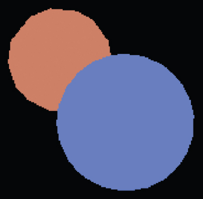
One problem with the minimal 3D pipeline is that in order to get occlusion relationships correct—to get nearer objects in front of farther away objects—primitives must be drawn in back-to-front order. This is known as the painter’s algorithm for hidden surface removal, by analogy to painting the background of a painting first, then painting the foreground over it. The painter’s algorithm is a perfectly valid way to remove hidden surfaces, but it has several drawbacks. It cannot handle triangles that intersect one another, because there is no correct order in which to draw them. Similarly, several triangles, even if they don’t intersect, can still be arranged in an occlusion cycle, as shown in Figure 8.9, another case in which the back-to-front order does not exist. And most importantly, sorting the primitives by depth is slow, especially for large scenes, and disturbs the efficient flow of data that makes object-order rendering so fast. Figure 8.10 shows the result of this process when the objects are not sorted by depth.

8.2.3 Using a z-Buffer for Hidden Surfaces

In practice, the painter’s algorithm is rarely used; instead a simple and effective hidden surface removal algorithm known as the z-buffer algorithm is used. The method is very simple: at each pixel we keep track of the distance to the closest surface that has been drawn so far, and we throw away fragments that are farther away than that distance. The closest distance is stored by allocating an extra value for each pixel, in addition to the red, green, and blue color values, which is known as the depth, or z-value. The depth buffer, or z-buffer, is the name for the grid of depth values.

The z-buffer algorithm is implemented in the fragment blending phase, by comparing the depth of each fragment with the current value stored in the z-buffer. If the fragment’s depth is closer, both its color and its depth value overwrite the values currently in the color and depth buffers. If the fragment’s depth is farther away, it is discarded. To ensure that the first fragment will pass the depth test, the z buffer is initialized to the maximum depth (the depth of the far plane). Irrespective of the order in which surfaces are drawn, the same fragment will win the depth test, and the image will be the same.

The z-buffer algorithm requires each fragment to carry a depth. This is done simply by interpolating the z-coordinate as a vertex attribute, in the same way that color or other attributes are interpolated.

The z-buffer is such a simple and practical way to deal with hidden surfaces in object-order rendering that it is by far the dominant approach. It is much simpler than geometric methods that cut surfaces into pieces that can be sorted by depth, because it avoids solving any problems that don’t need to be solved. The depth order only needs to be determined at the locations of the pixels, and that is all that the z-buffer does. It is universally supported by hardware graphics pipelines and is also the most commonly used method for software pipelines. Figure 8.11 shows an example result.

Precision Issues

In practice, the z-values stored in the buffer are nonnegative integers. This is preferable to true floats because the fast memory needed for the z-buffer is somewhat expensive and is worth keeping to a minimum.

The use of integers can cause some precision problems. If we use an integer range having B values {0, 1, . . . , B −1}, we can map 0 to the near clipping plane z = n and B −1 to the far clipping plane z = f. Note, that for this discussion, we assume z, n, and f are positive. This will result in the same results as the negative case, but the details of the argument are easier to follow. We send each z-value to a “bucket” with depth Δz = (f − n)/B. We would not use the integer z-buffer if memory were not a premium, so it is useful to make B as small as possible.

If we allocate b bits to store the z-value, then B = 2b. We need enough bits to make sure any triangle in front of another triangle will have its depth mapped to distinct depth bins.

For example, if you are rendering a scene where triangles have a separation of at least one meter, then Δz < 1 should yield images without artifacts. There are two ways to make Δz smaller: move n and f closer together or increase b. If b is fixed, as it may be in APIs or on particular hardware platforms, adjusting n and f is the only option.

The precision of z-buffers must be handled with great care when perspective images are created. The value Δz above is used after the perspective divide. Recall from Section 7.3 that the result of the perspective divide is

$z=n+f-\frac{fn}{z_w}.$

The actual bin depth is related to zw, the world depth, rather than z, the post-perspective divide depth. We can approximate the bin size by differentiating both sides:

$\Delta z\approx \frac{fn\Delta z_w}{z_w^2}.$

Bin sizes vary in depth. The bin size in world space is

$\Delta z_w\approx \frac{z_w^2\Delta z}{fn}.$

Note that the quantity Δz is as previously discussed. The biggest bin will be for z′ = f, where

$\Delta z_w^{\max }\approx \frac{f\Delta z}{n}.$

Note that choosing n = 0, a natural choice if we don’t want to lose objects right in front of the eye, will result in an infinitely large bin—a very bad condition. To make $\Delta z_w^{\max }$ as small as possible, we want to minimize f and maximize n. Thus, it is always important to choose n and f carefully.

8.2.4 Per-vertex Shading

So far the application sending triangles into the pipeline is responsible for setting the color; the rasterizer just interpolates the colors and they are written directly into the output image. For some applications this is sufficient, but in many cases we want 3D objects to be drawn with shading, using the same illumination equations that we used for image-order rendering in Chapter 4. Recall that these equations require a light direction, an eye direction, and a surface normal to compute the color of a surface.

One way to handle shading computations is to perform them in the vertex stage. The application provides normal vectors at the vertices, and the positions and colors of the lights are provided separately (they don’t vary across the surface, so they don’t need to be specified for each vertex). For each vertex, the direction to the viewer and the direction to each light are computed based on the positions of the camera, the lights, and the vertex. The desired shading equation is evaluated to compute a color, which is then passed to the rasterizer as the vertex color. Per-vertex shading is sometimes called Gouraud shading.

One decision to be made is the coordinate system in which shading computations are done. World space or eye space are good choices. It is important to choose a coordinate system that is orthonormal when viewed in world space, because shading equations depend on angles between vectors, which are not preserved by operations like nonuniform scale that are often used in the modeling transformation, or perspective projection, often used in the projection to the canonical view volume. Shading in eye space has the advantage that we don’t need to keep track of the camera position, because the camera is always at the origin in eye space, in perspective projection, or the view direction is always +z in orthographic projection.

Per-vertex shading has the disadvantage that it cannot produce any details in the shading that are smaller than the primitives used to draw the surface, because it only computes shading once for each vertex and never in between vertices. For instance, in a room with a floor that is drawn using two large triangles and illuminated by a light source in the middle of the room, shading will be evaluated only at the corners of the room, and the interpolated value will likely be much too dark in the center. Also, curved surfaces that are shaded with specular highlights must be drawn using primitives small enough that the highlights can be resolved.

Figure 8.13 shows our two spheres drawn with per-vertex shading.

8.2.5 Per-fragment Shading

To avoid the interpolation artifacts associated with per-vertex shading, we can avoid interpolating colors by performing the shading computations after the interpolation, in the fragment stage. In per-fragment shading, the same shading equations are evaluated, but they are evaluated for each fragment using interpolated vectors, rather than for each vertex using the vectors from the application.

In per-fragment shading, the geometric information needed for shading is passed through the rasterizer as attributes, so the vertex stage must coordinate with the fragment stage to prepare the data appropriately. One approach is to interpolate the eye-space surface normal and the eye-space vertex position, which then can be used just as they would in per-vertex shading.

Figure 8.14 shows our two spheres drawn with per-fragment shading.

8.2.6 Texture Mapping

Textures (discussed in Chapter 11) are images that are used to add extra detail to the shading of surfaces that would otherwise look too homogeneous and artificial. The idea is simple: each time shading is computed, we read one of the values used in the shading computation—the diffuse color, for instance—from a texture instead of using the attribute values that are attached to the geometry being rendered. This operation is known as a texture lookup: the shading code specifies a texture coordinate, a point in the domain of the texture, and the texture-mapping system finds the value at that point in the texture image and returns it. The texture value is then used in the shading computation.

The most common way to define texture coordinates is simply to make the texture coordinate another vertex attribute. Each primitive then knows where it lives in the texture.

8.2.7 Shading Frequency

The decision about where to place shading computations depends on how fast the color changes—the scale of the details being computed. Shading with large-scale features, such as diffuse shading on curved surfaces, can be evaluated fairly infrequently and then interpolated: it can be computed with a low shading frequency. Shading that produces small-scale features, such as sharp highlights or detailed textures, needs to be evaluated at a high shading frequency. For details that need to look sharp and crisp in the image, the shading frequency needs to be at least one shading sample per pixel.

So large-scale effects can safely be computed in the vertex stage, even when the vertices defining the primitives are many pixels apart. Effects that require a high shading frequency can also be computed at the vertex stage, as long as the vertices are close together in the image; alternatively, they can be computed at the fragment stage when primitives are larger than a pixel.

For example, a hardware pipeline as used in a computer game, generally using primitives that cover several pixels to ensure high efficiency, normally does most shading computations per fragment. On the other hand, the PhotoRealistic RenderMan system does all shading computations per vertex, after first subdividing, or dicing, all surfaces into small quadrilaterals called micropolygons that are about the size of pixels. Since the primitives are small, per-vertex shading in this system achieves a high shading frequency that is suitable for detailed shading.

8.3 Simple Antialiasing

Just as with ray tracing, rasterization will produce jagged lines and triangle edges if we make an all-or-nothing determination of whether each pixel is inside the primitive or not. In fact, the set of fragments generated by the simple triangle rasterization algorithms described in this chapter, sometimes called standard or aliased rasterization, is exactly the same as the set of pixels that would be mapped to that triangle by a ray tracer that sends one ray through the center of each pixel. Also as in ray tracing, the solution is to allow pixels to be partly covered by a primitive (Crow, 1978). In practice, this form of blurring helps visual quality, especially in animations. This is shown as the top line of Figure 8.15.

There are a number of different approaches to antialiasing in rasterization applications. Just as with a ray tracer, we can produce an antialiased image by setting each pixel value to the average color of the image over the square area belonging to the pixel, an approach known as box filtering. This means we have to think of all drawable entities as having well-defined areas. For example, the line in Figure 8.15 can be thought of as approximating a one-pixel-wide rectangle.

The easiest way to implement box-filter antialiasing is by supersampling: create images at very high resolutions and then downsample. For example, if our goal is a 256 × 256 pixel image of a line with width 1.2 pixels, we could rasterize a rectangle version of the line with width 4.8 pixels on a 1024 × 1024 screen, and then average 4 × 4 groups of pixels to get the colors for each of the 256 × 256 pixels in the “shrunken” image. This is an approximation of the actual box-filtered image, but works well when objects are not extremely small relative to the distance between pixels.

Supersampling is quite expensive, however. Because the very sharp edges that cause aliasing are normally caused by the edges of primitives, rather than sudden variations in shading within a primitive, a widely used optimization is to sample visibility at a higher rate than shading. If information about coverage and depth is stored for several points within each pixel, very good antialiasing can be achieved even if only one color is computed. In systems like RenderMan that use per-vertex shading, this is achieved by rasterizing at high resolution: it is inexpensive to do so because shading is simply interpolated to produce colors for the many fragments, or visibility samples. In systems with per-fragment shading, such as hardware pipelines, multisample antialiasing is achieved by storing for each fragment a single color plus a coverage mask and a set of depth values.

8.4 Culling Primitives for Efficiency

The strength of object-order rendering, that it requires a single pass over all the geometry in the scene, is also a weakness for complex scenes. For instance, in a model of an entire city, only a few buildings are likely to be visible at any given time. A correct image can be obtained by drawing all the primitives in the scene, but a great deal of effort will be wasted processing geometry that is behind the visible buildings, or behind the viewer, and therefore doesn’t contribute to the final image.

Identifying and throwing away invisible geometry to save the time that would be spent processing it is known as culling. Three commonly implemented culling strategies (often used in tandem) are

• view volume culling—the removal of geometry that is outside the view volume;
• occlusion culling—the removal of geometry that may be within the view volume but is obscured, or occluded, by other geometry closer to the camera;
• backface culling—the removal of primitives facing away from the camera.

We will briefly discuss view volume culling and backface culling, but culling in high performance systems is a complex topic; see (Akenine-Moöller et al., 2008) for a complete discussion and for information about occlusion culling.

8.4.1 View Volume Culling

When an entire primitive lies outside the view volume, it can be culled, since it will produce no fragments when rasterized. If we can cull many primitives with a quick test, we may be able to speed up drawing significantly. On the other hand, testing primitives individually to decide exactly which ones need to be drawn may cost more than just letting the rasterizer eliminate them.

View volume culling, also known as view frustum culling, is especially helpful when many triangles are grouped into an object with an associated bounding volume. If the bounding volume lies outside the view volume, then so do all the triangles that make up the object. For example, if we have 1000 triangles bounded by a single sphere with center c and radius r, we can check whether the sphere lies outside the clipping plane,

$\left(p-a\right)\cdot n=0,$

where a is a point on the plane, and p is a variable. This is equivalent to checking whether the signed distance from the center of the sphere c to the plane is greater than +r. This amounts to the check that

$\frac{\left(c-a\right)\cdot n}{||n||}>r.$

Note that the sphere may overlap the plane even in a case where all the triangles do lie outside the plane. Thus, this is a conservative test. How conservative the test is depends on how well the sphere bounds the object.

The same idea can be applied hierarchically if the scene is organized in one of the spatial data structures described in Chapter 12.

8.4.2 Backface Culling

When polygonal models are closed, i.e., they bound a closed space with no holes, then they are often assumed to have outward facing normal vectors as discussed in Chapter 10. For such models, the polygons that face away from the eye are certain to be overdrawn by polygons that face the eye. Thus, those polygons can be culled before the pipeline even starts. The test for this condition is the same one used for silhouette drawing given in Section 10.3.1.

Frequently Asked Questions

• I’ve often seen clipping discussed at length, and it is a much more involved process than that described in this chapter. What is going on here?

  The clipping described in this chapter works, but lacks optimizations that an industrial-strength clipper would have. These optimizations are discussed in detail in Blinn’s definitive work listed in the chapter notes.

• How are polygons that are not triangles rasterized?

  These can either be done directly scan-line by scan-line, or they can be broken down into triangles. The latter appears to be the more popular technique.

• Is it always better to antialias?

  No. Some images look crisper without antialiasing. Many programs use unantialiased “screen fonts” because they are easier to read.

• The documentation for my API talks about “scene graphs” and “matrix stacks.” Are these part of the graphics pipeline?

  The graphics pipeline is certainly designed with these in mind, and whether we define them as part of the pipeline is a matter of taste. This book delays their discussion until Chapter 12.

• Is a uniform distance z-buffer better than the standard one that includes perspective matrix nonlinearities?

  It depends. One “feature” of the nonlinearities is that the z-buffer has more resolution near the eye and less in the distance. If a level-of-detail system is used, then geometry in the distance is coarser and the “unfairness” of the z-buffer can be a good thing.

• Is a software z-buffer ever useful?

  Yes. Most of the movies that use 3D computer graphics have used a variant of the software z-buffer developed by Pixar (Cook, Carpenter, & Catmull, 1987).

Notes

A wonderful book about designing a graphics pipeline is Jim Blinn’s Corner: A Trip Down the Graphics Pipeline (J. Blinn, 1996). Many nice details of the pipeline and culling are in 3D Game Engine Design (Eberly, 2000) and Real-Time Rendering (Akenine-Moöller et al., 2008).

Exercises

1. Suppose that in the perspective transform we have n = 1 and f = 2. Under what circumstances will we have a “reversal” where a vertex before and after the perspective transform flips from in front of to behind the eye or vice versa?
2. Is there any reason not to clip in x and y after the perspective divide (see Figure 11.2, stage 3)?
3. Derive the incremental form of the midpoint line-drawing algorithm with colors at endpoints for 0 < m ≤ 1.
4. Modify the triangle-drawing algorithm so that it will draw exactly one pixel for points on a triangle edge which goes through (x, y) = (−1, −1).
5. Suppose you are designing an integer z-buffer for flight simulation where all of the objects are at least one meter thick, are never closer to the viewer than 4 meters, and may be as far away as 100 km. How many bits are needed in the z-buffer to ensure there are no visibility errors? Suppose that visibility errors only matter near the viewer, i.e., for distances less than 100 meters. How many bits are needed in that case?