Chapter 18

Light

In this chapter, we discuss the practical issues of measuring light, usually called radiometry. The terms that arise in radiometry may at first seem strange and have terminology and notation that may be hard to keep straight. However, because radiometry is so fundamental to computer graphics, it is worth studying radiometry until it sinks in. This chapter also covers photometry, which takes radiometric quantities and scales them to estimate how much “useful” light is present. For example, a green light may seem twice as bright as a blue light of the same power because the eye is more sensitive to green light. Photometry attempts to quantify such distinctions.

18.1 Radiometry

Although we can define radiometric units in many systems, we use SI (International System of Units) units. Familiar SI units include the metric units of meter (m) and gram (g). Light is fundamentally a propagating form of energy, so it is useful to define the SI unit of energy, which is the joule (J).

18.1.1 Photons

To aid our intuition, we will describe radiometry in terms of collections of large numbers of photons, and this section establishes what is meant by a photon in this context. For the purposes of this chapter, a photon is a quantum of light that has a position, direction of propagation, and a wavelength λ. Somewhat strangely, the SI unit used for wavelength is nanometer(nm). This is mainly for historical reasons, and 1 nm = 10−9 m. Another unit, the angstrom, is sometimes used, and one nanometer is ten angstroms. A photon also has a speed c that depends only on the refractive index n of the medium through which it propagates. Sometimes the frequency f = c/λ is also used for light. This is convenient because unlike λ and c, f does not change when the photon refracts into a medium with a new refractive index. Another invariant measure is the amount of energy q carried by a photon, which is given by the following relationship:

$q=hf=\frac{hc}{\text{λ}},\text{ (18.1)}$

where h = 6.63 × 10−34 J s is Plank’s Constant. Although these quantities can be measured in any unit system, we will use SI units whenever possible.

18.1.2 Spectral Energy

If we have a large collection of photons, their total energy Q can be computed by summing the energy qi of each photon. A reasonable question to ask is “How is the energy distributed across wavelengths?” An easy way to answer this is to partition the photons into bins, essentially histogramming them. We then have an energy associated with an interval. For example, we can count all the energy between λ = 500 nm and λ = 600 nm and have it turn out to be 10.2 J, and this might be denoted q[500, 600] = 10.2. If we divided the wavelength interval into two 50 nm intervals, we might find that q[500, 550] = 5.2 and q[550, 600] = 5.0. This tells us there was a little more energy in the short wavelength half of the interval [500, 600]. If we divide into 25 nm bins, we might find q [500, 525] = 2.5, and so on. The nice thing about the system is that it is straightforward. The bad thing about it is that the choice of the interval size determines the number.

A more commonly used system is to divide the energy by the size of the interval. So instead of q[500, 600] = 10.2 we would have

$Q_{\text{λ}}\left[500,600\right]=\frac{10.2}{100}=0.12 \mathbf{\text{J}}{\left(\text{nm}\right)}^{-1}.$

This approach is nice, because the size of the interval has much less impact on the overall size of the numbers. An immediate idea would be to drive the interval size Δλ to zero. This could be awkward, because for a sufficiently small Δλ, Qλ will either be zero or huge depending on whether there is a single photon or no photon in the interval. There are two schools of thought to solve that dilemma. The first is to assume that Δλ is small, but not so small that the quantum nature of light comes into play. The second is to assume that the light is a continuum rather than individual photons, so a true derivative dQ/dλ is appropriate. Both ways of thinking about it are appropriate and lead to the same computational machinery. In practice, it seems that most people who measure light prefer small, but finite, intervals, because that is what they can measure in the lab. Most people who do theory or computation prefer infinitesimal intervals, because that makes the machinery of calculus available.

The quantity Qλ is called spectral energy, and it is an intensive quantity as opposed to an extensive quantity such as energy, length, or mass. Intensive quantities can be thought of as density functions that tell the density of an extensive quantity at an infinitesimal point. For example, the energy Q at a specific wavelength is probably zero, but the spectral energy (energy density) Qλ is a meaningful quantity. A probably more familiar example is that the population of a country may be 25 million, but the population at a point in that country is meaningless. However, the population density measured in people per square meter is meaningful, provided it is measured over large enough areas. Much like with photons, population density works best if we pretend that we can view population as a continuum where population density never becomes granular even when the area is small.

We will follow the convention of graphics where spectral energy is almost always used, and energy is rarely used. This results in a proliferation of λ subscripts if “proper” notation is used. Instead, we will drop the subscript and use Q to denote spectral energy. This can result in some confusion when people outside of graphics read graphics papers, so be aware of this standards issue. Your intuition about spectral energy might be aided by imagining a measurement device with a sensor that measures light energy Δq. If you place a colored filter in front of the sensor that allows only light in the interval [λ − Δλ/2, λ + Δλ/2], then the spectral energy at λ is Q = Δq/Δλ.

18.1.3 Power

It is useful to estimate a rate of energy production for light sources. This rate is called power, and it is measured in watts, W, which is another name for joules per second. This is easiest to understand in a steady state, but because power is an intensive quantity (a density over time), it is well defined even when energy production is varying over time. The units of power may be more familiar, e.g., a 100-watt light bulb. Such bulbs draw approximately 100 J of energy each second. The power of the light produced will actually be less than 100 W because of heat loss, etc., but we can still use this example to help understand more about photons. For example, we can get a feel for how many photons are produced in a second by a 100 W light. Suppose the average photon produced has the energy of a λ = 500 nm photon. The frequency of such a photon is

$f=\frac{c}{\lambda }=\frac{3\times {10}^8{\text{ms}}^{-1}}{500\times {10}^{-9}\text{m}}=6\times {10}^{14}{\text{s}}^{-\text{1}}.$

The energy of that photon is hf ≈ 4 × 10−19 J. That means a staggering 1020 photons are produced each second, even if the bulb is not very efficient. This explains why simulating a camera with a fast shutter speed and directly simulated photons is an inefficient choice for producing images.

As with energy, we are really interested in spectral power measured in W(nm)−1. Again, although the formal standard symbol or spectral power is ΦΔ, we will use Φ with no subscript for convenience and consistency with most of the graphics literature. One thing to note is that the spectral power for a light source is usually a smaller number than the power. For example, if a light emits a power of 100 W evenly distributed over wavelengths 400 nm to 800 nm, then the spectral power will be 100 W/400 nm = 0.25 W(nm)−1. This is something to keep in mind if you set the spectral power of light sources by hand for debugging purposes.

The measurement device for spectral energy in the last section could be modified by taking a reading with a shutter that is open for a time interval Δt centered at time t. The spectral power would then be Φ = Δq/(ΔtΔλ).

18.1.4 Irradiance

The quantity irradiance arises naturally if you ask the question “How much light hits this point?” Of course the answer is “none,” and again we must use a density function. If the point is on a surface, it is natural to use area to define our density function. We modify the device from the last section to have a finite ΔA area sensor that is smaller than the light field being measured. The spectral irradiance H is just the power per unit area ΔΦ/ΔA. Fully expanded this is

$H=\frac{\Delta q}{\Delta A\Delta t\Delta \lambda }.\text{ (18.2)}$

Thus, the full units of irradiance are Jm−2 s−1(nm)−1. Note that the SI units for radiance include inverse-meter-squared for area and inverse-nanometer for wavelength. This seeming inconsistency (using both nanometer and meter) arises because of the natural units for area and visible light wavelengths.

When the light is leaving a surface, e.g., when it is reflected, the same quantity as irradiance is called radiant exitance, E. It is useful to have different words for incident and exitant light, because the same point has potentially different irradiance and radiant exitance.

18.1.5 Radiance

Although irradiance tells us how much light is arriving at a point, it tells us little about the direction that light comes from. To measure something analogous to what we see with our eyes, we need to be able to associate “how much light” with a specific direction. We can imagine a simple device to measure such a quantity (Figure 18.1). We use a small irradiance meter and add a conical “baffler” which limits light hitting the counter to a range of angles with solid angle Δσ. The response of the detector is as follows:

$\begin{array}{cc}\hfill \text{response}& =\frac{\Delta H}{\Delta \sigma }\hfill \\ \hfill & =\frac{\Delta q}{\Delta A\Delta \sigma \Delta t\Delta \text{λ}}.\hfill \end{array}$

This is the spectral radiance of light traveling in space. Again, we will drop the “spectral” in our discussion and assume that it is implicit.

Radiance is what we are usually computing in graphics programs. A wonderful property of radiance is that it does not vary along a line in space. To see why this is true, examine the two radiance detectors both looking at a surface as shown in Figure 18.2. Assume the lines the detectors are looking along are close enough together that the surface is emitting/reflecting light “the same” in both of the areas being measured. Because the area of the surface being sampled is proportional to squared distance, and because the light reaching the detector is inversely proportional to squared distance, the two detectors should have the same reading.

It is useful to measure the radiance hitting a surface. We can think of placing the cone baffler from the radiance detector at a point on the surface and measuring the irradiance H on the surface originating from directions within the cone (Figure 18.3). Note that the surface “detector” is not aligned with the cone. For this reason we need to add a cosine correction term to our definition of radiance:

$\begin{array}{cc}\hfill \text{response}& =\frac{\Delta H}{\Delta \sigma \cos \theta }\hfill \\ \hfill & =\frac{\Delta q}{\Delta A\cos \theta \Delta \sigma \Delta t\Delta \text{λ}}.\hfill \end{array}$

As with irradiance and radiant exitance, it is useful to distinguish between radiance incident at a point on a surface and exitant from that point. Terms for these concepts sometimes used in the graphics literature are surface radiance Ls for the radiance of (leaving) a surface, and field radiance Lf for the radiance incident at a surface. Both require the cosine term, because they both correspond to the configuration in Figure 18.3:

$\begin{array}{cc}\hfill L_s& =\frac{\Delta E}{\Delta \sigma \cos \theta }\hfill \\ \hfill L_f& =\frac{\Delta H}{\Delta \sigma \cos \theta }.\hfill \end{array}$

Radiance and Other Radiometric Quantities

If we have a surface whose field radiance is Lf, then we can derive all of the other radiometric quantities from it. This is one reason radiance is considered the “fundamental” radiometric quantity. For example, the irradiance can be expressed as

$H={\displaystyle {\int }_{\text{all}k}{L}_f\left(k\right)\cos \theta d\sigma .}$

This formula has several notational conventions that are common in graphics that make such formulae opaque to readers not familiar with them (Figure 18.4). First, k is an incident direction and can be thought of as a unit vector, a direction, or a (θ, ϕ) pair in spherical coordinates with respect to the surface normal. The direction has a differential solid angle dσ associated with it. The field radiance is potentially different for every direction, so we write it as a function L(k).

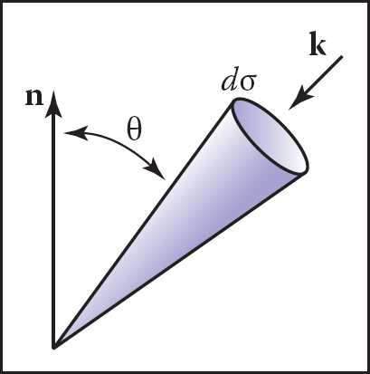
As an example, we can compute the irradiance H at a surface that has constant field radiance Lf in all directions. To integrate, we use a classic spherical coordinate system and recall that the differential solid angle is

$d\sigma \equiv \sin \theta d\theta d\varphi ,$

so the irradiance is

$\begin{array}{cc}\hfill H& ={\displaystyle {\int }_{\varphi =0}^{2\pi }{\displaystyle {\int }_{\theta =0}^{\frac{\pi }{2}}{L}_f}\cos \theta \sin \theta d\theta d\varphi }\hfill \\ \hfill & =\pi L_f.\hfill \end{array}$

This relation shows us our first occurrence of a potentially surprising constant π. These factors of π occur frequently in radiometry and are an artifact of how we chose to measure solid angles, i.e., the area of a unit sphere is a multiple of π rather than a multiple of one.

Similarly, we can find the power hitting a surface by integrating the irradiance across the surface area:

$\Phi ={\displaystyle {\int }_{\text{all}\text{x}}H\left(x\right)dA,}$

where x is a point on the surface, and dA is the differential area associated with that point. Note that we don’t have special terms or symbols for incoming versus outgoing power. That distinction does not seem to come up enough to have encouraged the distinction.

18.1.6 BRDF

Because we are interested in surface appearance, we would like to characterize how a surface reflects light. At an intuitive level, for any incident light coming from direction ki, there is some fraction scattered in a small solid angle near the outgoing direction ko. There are many ways we could formalize such a concept, and not surprisingly, the standard way to do so is inspired by building a simple measurement device. Such a device is shown in Figure 18.5, where a small light source is positioned in direction ki as seen from a point on a surface, and a detector is placed in direction ko. For every directional pair (ki, ko), we take a reading with the detector.

Now we just have to decide how to measure the strength of the light source and make our reflection function independent of this strength. For example, if we replaced the light with a brighter light, we would not want to think of the surface as reflecting light differently. We could place a radiance meter at the point being illuminated to measure the light. However, for this to get an accurate reading that would not depend on the Δσ of the detector, we would need the light to subtend a solid angle bigger than Δσ. Unfortunately, the measurement taken by our roving radiance detector in direction ko will also count light that comes from points outside the new detector’s cone. So this does not seem like a practical solution.

Alternatively, we can place an irradiance meter at the point on the surface being measured. This will take a reading that does not depend strongly on subtleties of the light source geometry. This suggests characterizing reflectance as a ratio:

$\rho =\frac{L_s}{H},$

where this fraction ρ will vary with incident and exitant directions ki and ko, H is the irradiance for light position ki, and Ls is the surface radiance measured in direction ko. If we take such a measurement for all direction pairs, we end up with a 4D function ρ(ki, ko). This function is called the bidirectional reflectance distribution function (BRDF). The BRDF is all we need to know to characterize the directional properties of how a surface reflects light.

Directional Hemispherical Reflectance

Given a BRDF, it is straightforward to ask, “What fraction of incident light is reflected?” However, the answer is not so easy; the fraction reflected depends on the directional distribution of incoming light. For this reason, we typically only set a fraction reflected for a fixed incident direction ki. This fraction is called the directional hemispherical reflectance. This fraction, R(ki) is defined by

$R\left(k_i\right)=\frac{\text{power}\text{in}\text{all}\text{outgoing}\text{directions}{k}_o}{\text{power}\text{in}\text{a}\text{beam}\text{from}\text{direction}{k}_i}.$

Note that this quantity is between zero and one for reasons of energy conservation. If we allow the incident power Φi to hit on a small area ΔA, then the irradiance is Φi/ΔA. Also, the ratio of the incoming power is just the ratio of the radiant exitance to irradiance:

$R\left(k_i\right)=\frac{E}{H}.$

The radiance in a particular direction resulting from this power is by the definition of BRDF:

$\begin{array}{cc}\hfill L\left(k_o\right)& =H\rho \left(k_i,k_o\right)\hfill \\ \hfill & =\frac{{\Phi }_i}{\Delta A}.\hfill \end{array}$

And from the definition of radiance, we also have

$L\left(k_o\right)=\frac{\Delta E}{\Delta {\sigma }_o\cos {\theta }_o},$

where E is the radiant exitance of the small patch in direction ko. Using these two definitions for radiance we get

$H\rho \left(k_i,k_o\right)=\frac{\Delta E}{\Delta {\sigma }_o\cos {\theta }_o}.$

Rearranging terms, we get

$\frac{\Delta E}{H}=\rho \left(k_i,k_o\right)\Delta {\sigma }_o\cos {\theta }_o.$

This is just the small contribution to E/H that is reflected near the particular ko. To find the total R(ki), we sum over all outgoing ko. In integral form this is

$R\left(k_i\right)={\displaystyle {\int }_{\text{all}{k}_o}\rho \left(k_i,k_o\right)\cos {\theta }_{o}d{\sigma }_o.}$

Ideal Diffuse BRDF

An idealized diffuse surface is called Lambertian. Such surfaces are impossible in nature for thermodynamic reasons, but mathematically they do conserve energy. The Lambertian BRDF has ρ equal to a constant for all angles. This means the surface will have the same radiance for all viewing angles, and this radiance will be proportional to the irradiance.

If we compute R(ki) for a a Lambertian surface with ρ = C we get

$\begin{array}{cc}\hfill R\left(k_i\right)& ={\displaystyle {\int }_{\text{all}{k}_o}C\cos {\theta }_{o}d{\sigma }_o}\hfill \\ \hfill & ={\displaystyle {\int }_{{\varphi }_o=0}^{2\pi }{\displaystyle {\int }_{{\theta }_o=0}^{\pi /2}C\cos {\theta }_o\sin {\theta }_{o}d{\theta }_{o}d{\varphi }_o}}\hfill \\ \hfill & =\pi C.\hfill \end{array}$

Thus, for a perfectly reflecting Lambertian surface (R = 1), we have ρ = 1/π, and for a Lambertian surface where R(ki) = r, we have

$\rho \left(k_i,k_o\right)=\frac{r}{\pi }.$

This is another example where the use of a steradian for the solid angle determines the normalizing constant and thus introduces factors of π.

18.2 Transport Equation

With the definition of BRDF, we can describe the radiance of a surface in terms of the incoming radiance from all different directions. Because in computer graphics we can use idealized mathematics that might be impractical to instantiate in the lab, we can also write the BRDF in terms of radiance only. If we take a small part of the light with solid angle Δσi with radiance Li and “measure” the reflected radiance in direction ko due to this small piece of the light, we can compute a BRDF (Figure 18.6). The irradiance due to the small piece of light is H = Li cosθiΔσi. Thus the BRDF is

$\rho =\frac{L_o}{L_i\cos {\theta }_i\Delta {\sigma }_i}.$

This form can be useful in some situations. Rearranging terms, we can write down the part of the radiance that is due to light coming from direction ki:

$\Delta L_o=\rho \left(k_i,k_o\right)L_i\cos {\theta }_i\Delta {\sigma }_i.$

If there is light coming from many directions Li(ki), we can sum all of them. In integral form, with notation for surface and field radiance, this is

$L_s\left(k_o\right)={\displaystyle {\int }_{\text{all}{k}_i}\rho \left(k_i,k_o\right)L_f\left(k_i\right)\cos {\theta }_{i}d{\sigma }_i.}$

This is often called the rendering equation in computer graphics (Immel, Cohen, & Greenberg, 1986).

Sometimes it is useful to write the transport equation in terms of surface radiances only (Kajiya, 1986). Note, that in a closed environment, the field radiance Lf (ki) comes from some surface with surface radiance Ls(−ki) = Lf(ki) (Figure 18.7). The solid angle subtended by the point x' in the figure is given by

$\Delta {\sigma }_i=\frac{\Delta A^{\prime }\cos {\theta }^{\prime }}{{||x-{\text{x}}^{\prime }||}^2},$

where ΔA' the the area we associate with x'. Substituting for Δσi in terms of ΔA' suggests the following transport equation:

$L_s\left(\text{x,}{k}_o\right)={\displaystyle {\int }_{\text{all}\text{x'}\text{visible}\text{to x}}\frac{\rho \left(k_i,k_o\right)L_s\left({\text{x}}^{\prime },x-{\text{x}}^{\prime }\right)\cos {\theta }_i\cos {\theta }^{\prime }}{{||x-{\text{x}}^{\prime }||}^2}d{A}^{\prime }}.$

Note that we are using a non-normalized vector x – x' to indicate the direction from x' to x. Also note that we are writing Ls as a function of position and direction.

The only problem with this new transport equation is that the domain of integration is awkward. If we introduce a visibility function, we can trade off complexity in the domain with complexity in the integrand:

$L_s\left(\mathbf{\text{x}},k_o\right)={\displaystyle {\int }_{\text{all}\text{x}}\frac{\rho \left({\mathbf{k}}_i,k_o\right)L_s\left({\mathbf{\text{x}}}^{\prime },\mathbf{x}-{\mathbf{\text{x}}}^{\prime }\right)v\left(\text{x,}{\mathbf{\text{x}}}^{\prime }\right)\cos {\theta }_i\cos {\theta }^{\prime }}{{||x-{\mathbf{\text{x}}}^{\prime }||}^2}d{A}^{\prime }},$

where

$v\left(\mathbf{\text{x}},{\mathbf{\text{x}}}^{\prime }\right)=\{\begin{array}{ll}1\hfill & \text{if}\mathbf{x}\text{and}\mathbf{\text{x}}\text{are mutually}\text{visible,}\hfill \\ 0\hfill & \text{otherwise}\text{.}\hfill \end{array}$

18.3 Photometry

For every spectral radiometric quantity there is a related photometric quantity that measures how much of that quantity is “useful” to a human observer. Given a spectral radiometric quantity fr(λ), the related photometric quantity fp is

$f_p=683\frac{\text{lm}}{W}{\displaystyle {\int }_{\text{λ=380}\text{nm}}^{800\text{nm}}\overline{y}}\left(\text{λ}\right)f_r\left(\text{λ}\right)d\text{λ,}$

where $\overline{y}$ is the luminous efficiency function of the human visual system. This function is zero outside the limits of integration above, so the limits could be 0 and ∞ and fp would not change. The luminous efficiency function will be discussed in more detail in Chapter 19, but we discuss its general properties here. The leading constant is to make the definition consistent with historical absolute photometric quantities.

The luminous efficiency function is not equally sensitive to all wavelengths (Figure 18.8). For wavelengths below 380 nm (the ultraviolet range), the light is not visible to humans and thus has a $\overline{y}$ value of zero. From 380 nm it gradually increases until λ = 555 nm where it peaks. This is a pure green light. Then, it gradually decreases until it reaches the boundary of the infrared region at 800 nm.

The photometric quantity that is most commonly used in graphics is luminance, the photometric analog of radiance:

$Y=683\frac{\text{lm}}{W}{\displaystyle {\int }_{\text{λ=380}\text{nm}}^{800\text{nm}}\overline{y}}\left(\text{λ}\right)L\left(\text{λ}\right)d\text{λ}\text{.}$

The symbol Y for luminance comes from colorimetry. Most other fields use the symbol L; we will not follow that convention because it is too confusing to use L for both luminance and spectral radiance. Luminance gives one a general idea of how “bright” something is independent of the adaptation of the viewer. Note that the black paper under noonday sun is subjectively darker than the lower luminance white paper under moonlight; reading too much into luminance is dangerous, but it is a very useful quantity for getting a quantitative feel for relative perceivable light output. The unit lm stands for lumens. Note that most light bulbs are rated in terms of the power they consume in watts, and the useful light they produce in lumens. More efficient bulbs produce more of their light where $\overline{y}$ is large and thus produce more lumens per watt. A “perfect” light would convert all power into 555 nm light and would produce 683 lumens per watt. The units of luminance are thus (lm/W)(W/(m2sr)) = lm/(m2sr). The quantity one lumen per steradian is defined to be one candela(cd), so luminance is usually described in units cd/m2.

Frequently Asked Questions

• What is “intensity”?

  The term intensity is used in a variety of contexts and its use varies with both era and discipline. In practice, it is no longer meaningful as a specific radiometric quantity, but it is useful for intuitive discussion. Most papers that use it do so in place of radiance.

• What is “radiosity”?

  The term radiosity is used in place of radiant exitance in some fields. It is also sometimes used to describe world-space light transport algorithms.

Notes

A common radiometric quantity not described in this chapter is radiant intensity (I), which is the spectral power per steradian emitted from an infinitesimal point source. It should usually be avoided in graphics programs because point sources cause implementation problems. A more rigorous treatment of radiometry can be found in Analytic Methods for Simulated Light Transport (Arvo, 1995). The radiometric and photometric terms in this chapter are from the Illumination Engineering Society’s standard that is increasingly used by all fields of science and engineering (American National Standard Institute, 1986). A broader discussion of radiometric and appearance standards can be found in Principles of Digital Image Synthesis (Glassner, 1995).

Exercises

1. For a diffuse surface with outgoing radiance L, what is the radiant exitance?
2. What is the total power exiting a diffuse surface with an area of 4 m2 and a radiance of L?
3. If a fluorescent light and an incandescent light both consume 20 watts of power, why is the fluorescent light usually preferred?