
Chapter 12
Data Structures for Graphics
Certain data structures seem to pop up repeatedly in graphics applications, perhaps because they address fundamental underlying ideas like surfaces, space, and scene structure. This chapter talks about several basic and unrelated categories of data structures that are among the most common and useful: mesh structures, spatial data structures, scene graphs, and tiled multidimensional arrays.
For meshes, we discuss the basic storage schemes used for storing static meshes and for transferring meshes to graphics APIs. We also discuss the winged-edge data structure (Baumgart, 1974) and the related half-edge structure, which are useful for managing models where the tessellation changes, such as in subdivision or model simplification. Although these methods generalize to arbitrary polygon meshes, we focus on the simpler case of triangle meshes here.
Next, the scene-graph data structure is presented. Various forms of this data structure are ubiquitous in graphics applications because they are so useful in managing objects and transformations. All new graphics APIs are designed to support scene graphs well.
For spatial data structures, we discuss three approaches to organizing models in 3D space—bounding volume hierarchies, hierarchical space subdivision, and uniform space subdivision—and the use of hierarchical space subdivision (BSP trees) for hidden surface removal. The same methods are also used for other purposes, including geometry culling and collision detection.
Finally, the tiled multidimensional array is presented. Originally developed to help paging performance in applications where graphics data needed to be swapped in from disk, such structures are now crucial for memory locality on machines regardless of whether the array fits in main memory.
12.1 Triangle Meshes
Most real-world models are composed of complexes of triangles with shared vertices. These are usually known as triangular meshes, triangle meshes, or triangular irregular networks (TINs), and handling them efficiently is crucial to the performance of many graphics programs. The kind of efficiency that is important depends on the application. Meshes are stored on disk and in memory, and we’d like to minimize the amount of storage consumed. When meshes are transmitted across networks or from the CPU to the graphics system, they consume bandwidth, which is often even more precious than storage. In applications that perform operations on meshes, besides simply storing and drawing them—such as subdivision, mesh editing, mesh compression, or other operations—efficient access to adjacency information is crucial.
Triangle meshes are generally used to represent surfaces, so a mesh is not just a collection of unrelated triangles, but rather a network of triangles that connect to one another through shared vertices and edges to form a single continuous surface. This is a key insight about meshes: a mesh can be handled more efficiently than a collection of the same number of unrelated triangles.
The minimum information required for a triangle mesh is a set of triangles (triples of vertices) and the positions (in 3D space) of their vertices. But many, if not most, programs require the ability to store additional data at the vertices, edges, or faces to support texture mapping, shading, animation, and other operations. Vertex data is the most common: each vertex can have material parameters, texture coordinates, irradiances—any parameters whose values change across the surface. These parameters are then linearly interpolated across each triangle to define a continuous function over the whole surface of the mesh. However, it is also occasionally important to be able to store data per edge or per face.
12.1.1 Mesh Topology
The idea that meshes are surface-like can be formalized as constraints on the mesh topology—the way the triangles connect together, without regard for the vertex positions. Many algorithms will only work, or are much easier to implement, on a mesh with predictable connectivity. The simplest and most restrictive requirement on the topology of a mesh is for the surface to be a manifold. A manifold mesh is “watertight”—it has no gaps and separates the space on the inside of the surface from the space outside. It also looks like a surface everywhere on the mesh.
The term manifold comes from the mathematical field of topology: roughly speaking, a manifold (specifically a two-dimensional manifold, or 2-manifold) isa surface in which a small neighborhood around any point could be smoothed out into a bit of flat surface. This idea is most clearly explained by counterexample: if an edge on a mesh has three triangles connected to it, the neighborhood of a point on the edge is different from the neighborhood of one of the points in the interior of one of the triangles, because it has an extra “fin” sticking out of it (Figure 12.1). If the edge has exactly two triangles attached to it, points on the edge have neighborhoods just like points in the interior, only with a crease down the middle. Similarly, if the triangles sharing a vertex are in a configuration like the left one in Figure 12.2, the neighborhood is like two pieces of surface glued together at the center, which can’t be flattened without doubling it up. The vertex with the simpler neighborhood shown at right is just fine.


Many algorithms assume that meshes are manifold, and it’s always a good idea to verify this property to prevent crashes or infinite loops if you are handed a malformed mesh as input. This verification boils down to checking that all edges are manifold and checking that all vertices are manifold by verifying the following conditions:
- Every edge is shared by exactly two triangles.
- Every vertex has a single, complete loop of triangles around it.
Figure 12.1 illustrates how an edge can fail the first test by having too many triangles, and Figure 12.2 illustrates how a vertex can fail the second test by having two separate loops of triangles attached to it.
Manifold meshes are convenient, but sometimes it’s necessary to allow meshes to have edges, or boundaries. Such meshes are not manifolds—a point on the boundary has a neighborhood that is cut off on one side. They are not necessarily watertight. However, we can relax the requirements of a manifold mesh to those for a manifold with boundary without causing problems for most mesh processing algorithms. The relaxed conditions are:
- Every edge is used by either one or two triangles.
- Every vertex connects to a single edge-connected set of triangles.
Figure 12.3 illustrates these conditions: from left to right, there is an edge with one triangle, a vertex whose neighboring triangles are in a single edge-connected set, and a vertex with two disconnected sets of triangles attached to it.

Finally, in many applications it’s important to be able to distinguish the “front” or “outside” of a surface from the “back” or “inside”—this is known as the orientation of the surface. For a single triangle, we define orientation based on the order in which the vertices are listed: the front is the side from which the triangle’s three vertices are arranged in counterclockwise order. A connected mesh is consistently oriented if its triangles all agree on which side is the front—and this is true if and only if every pair of adjacent triangles is consistently oriented.
In a consistently oriented pair of triangles, the two shared vertices appear in opposite orders in the two triangles’ vertex lists (Figure 12.4). What’s important is consistency of orientation—some systems define the front using clockwise rather than counterclockwise order.

Triangles (B,A,C) and (D,C,A) are consistently oriented, whereas (B,A,C) and (A,C,D) are inconsistently oriented.
Any mesh that has non-manifold edges can’t be oriented consistently. But it’s also possible for a mesh to be a valid manifold with boundary (or even a manifold), and yet have no consistent way to orient the triangles—they are not orientable surfaces. An example is the Moöbius band shown in Figure 12.5. This is rarely an issue in practice, however.

12.1.2 Indexed Mesh Storage
A simple triangular mesh is shown in Figure 12.6. You could store these three triangles as independent entities, each of this form:

A three-triangle mesh with four vertices, represented with separate triangles (left) and with shared vertices (right).
Triangle {
vector3 vertexPosition[3]
}
This would result in storing vertex b three times and the other vertices twice each for a total of nine stored points (three vertices for each of three triangles). Or you could instead arrange to share the common vertices and store only four, resulting in a shared-vertex mesh. Logically, this data structure has triangles which point to vertices which contain the vertex data:
Triangle {
Vertex v[3]
}
Vertex {
vector3 position // or other vertex data
}
Note that the entries in the v array are references, or pointers, to Vertex objects; the vertices are not contained in the triangle.
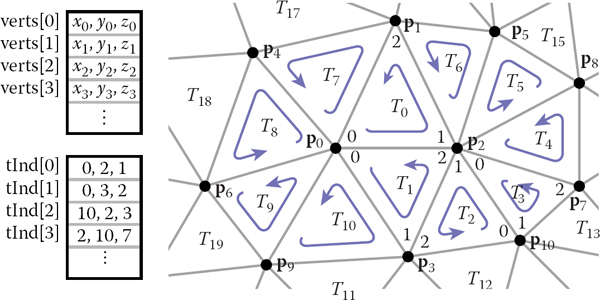
In implementation, the vertices and triangles are normally stored in arrays, with the triangle-to-vertex references handled by storing array indices:
IndexedMesh {
int tInd[nt][3]
vector3 verts[nv]
}
The index of the kth vertex of the ith triangle is found in tInd[i][k], and the position of that vertex is stored in the corresponding row of the verts array; see Figure 12.8 for an example. This way of storing a shared-vertex mesh is an indexed triangle mesh.

Separate triangles or shared vertices will both work well. Is there a space advantage for sharing vertices? If our mesh has nv vertices and nt triangles, and if we assume that the data for floats, pointers, and ints all require the same storage (a dubious assumption), the space requirements are as follows:
- Triangle. Three vectors per triangle, for 9nt units of storage;
- IndexedMesh. One vector per vertex and three ints per triangle, for 3nv + 3nt units of storage.
The relative storage requirements depend on the ratio of nt to nv.
As a rule of thumb, a large mesh has each vertex connected to about six triangles (although there can be any number for extreme cases). Since each triangle connects to three vertices, this means that there are generally twice as many triangles as vertices in a large mesh: nt ≈ 2nv. Making this substitution, we can conclude that the storage requirements are 18nv for the Triangle structure and 9nv for IndexedMesh. Using shared vertices reduces storage requirements by about a factor of two; and this seems to hold in practice for most implementations.
12.1.3 Triangle Strips and Fans
Indexed meshes are the most common in-memory representation of triangle meshes, because they achieve a good balance of simplicity, convenience, and compactness. They are also commonly used to transfer meshes over networks and between the application and graphics pipeline. In applications where even more compactness is desirable, the triangle vertex indices (which take up two-thirds of the space in an indexed mesh with only positions at the vertices) can be expressed more efficiently using triangle strips and triangle fans.
A triangle fan is shown in Figure 12.9. In an indexed mesh, the triangles array would contain [(0, 1, 2), (0, 2, 3), (0, 3, 4), (0, 4, 5)]. We are storing 12 vertex indices, although there are only six distinct vertices. In a triangle fan, all the triangles share one common vertex, and the other vertices generate a set of triangles like the vanes of a collapsible fan. The fan in the figure could be specified with the sequence [0, 1, 2, 3, 4, 5]: the first vertex establishes the center, and subsequently each pair of adjacent vertices (1-2, 2-3, etc.) creates a triangle.

The triangle strip is a similar concept, but it is useful for a wider range of meshes. Here, vertices are added alternating top and bottom in a linear strip as shown in Figure 12.10. The triangle strip in the figure could be specified by the sequence [0 1 2 3 4 5 6 7], and every subsequence of three adjacent vertices (0-1-2, 1-2-3, etc.) creates a triangle. For consistent orientation, every other triangle needs to have its order reversed. In the example, this results in the triangles (0, 1, 2), (2, 1, 3), (2, 3, 4), (4, 3, 5), etc. For each new vertex that comes in, the oldest vertex is forgotten and the order of the two remaining vertices is swapped. See Figure 12.11 for a larger example.


Two triangle strips in the context of a larger mesh. Note that neither strip can be extended to include the triangle marked with an asterisk.
In both strips and fans, n + 2 vertices suffice to describe n triangles—a substantial savings over the 3n vertices required by a standard indexed mesh. Long triangle strips will save approximately a factor of three if the program is vertex-bound.
It might seem that triangle strips are only useful if the strips are very long, but even relatively short strips already gain most of the benefits. The savings in storage space (for only the vertex indices) are as follows:
strip length |
1 |
2 |
3 |
4 |
5 |
6 |
7 |
8 |
16 |
100 |
∞ |
relative size |
1.00 |
0.67 |
0.56 |
0.50 |
0.47 |
0.44 |
0.43 |
0.42 |
0.38 |
0.34 |
0.33 |
So, in fact, there is a rather rapid diminishing return as the strips grow longer. Thus, even for an unstructured mesh, it is worthwhile to use some greedy algorithm to gather them into short strips.
12.1.4 Data Structures for Mesh Connectivity
Indexed meshes, strips, and fans are all good, compact representations for static meshes. However, they do not readily allow for meshes to be modified. In order to efficiently edit meshes, more complicated data structures are needed to efficiently answer queries such as:
- Given a triangle, what are the three adjacent triangles?
- Given an edge, which two triangles share it?
- Given a vertex, which faces share it?
- Given a vertex, which edges share it?
There are many data structures for triangle meshes, polygonal meshes, and polygonal meshes with holes (see the notes at the end of the chapter for references). In many applications the meshes are very large, so an efficient representation can be crucial.
The most straightforward, though bloated, implementation would be to have three types, Vertex, Edge, and Triangle, and to just store all the relationships directly:
Triangle {
Vertex v[3]
Edge e[3]
}
Edge {
Vertex v[2]
Triangle t[2]
}
Vertex {
Triangle t[]
Edge e[]
}
This lets us directly look up answers to the connectivity questions above, but because this information is all inter-related, it stores more than is really needed. Also, storing connectivity in vertices makes for variable-length data structures (since vertices can have arbitrary numbers of neighbors), which are generally less efficient to implement. Rather than committing to store all these relationships explicitly, it is best to define a class interface to answer these questions, behind which a more efficient data structure can hide. It turns out we can store only some of the connectivity and efficiently recover the other information when needed.
The fixed-size arrays in the Edge and Triangle classes suggest that it will be more efficient to store the connectivity information there. In fact, for polygon meshes, in which polygons have arbitrary numbers of edges and vertices, only edges have fixed-size connectivity information, which leads to many traditional mesh data structures being based on edges. But for triangle-only meshes, storing connectivity in the (less numerous) faces is appealing.
A good mesh data structure should be reasonably compact and allow efficient answers to all adjacency queries. Efficient means constant-time: the time to find neighbors should not depend on the size of the mesh. We’ll look at three data structures for meshes, one based on triangles and two based on edges.
The Triangle-Neighbor Structure
We can create a compact mesh data structure based on triangles by augmenting the basic shared-vertex mesh with pointers from the triangles to the three neighboring triangles, and a pointer from each vertex to one of the adjacent triangles (it doesn’t matter which one); see Figure 12.12:
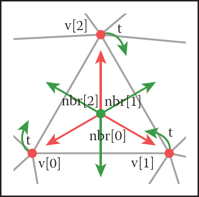
Triangle {
Triangle nbr[3];
Vertex v[3];
}
Vertex {
// ... per-vertex data ...
Triangle t; // any adjacent tri
}
In the array Triangle.nbr, the kth entry points to the neighboring triangle that shares vertices k and k + 1. We call this structure the triangle-neighbor structure. Starting from standard indexed mesh arrays, it can be implemented with two additional arrays: one that stores the three neighbors of each triangle, and one that stores a single neighboring triangle for each vertex (see Figure 12.13 for an example):

The triangle-neighbor structure as encoded in arrays, and the sequence that is followed in traversing the neighboring triangles of vertex 2.
Mesh {
// ... per-vertex data ...
int tInd[nt][3]; // vertex indices
int tNbr[nt][3]; // indices of neighbor triangles
int vTri[nv]; // index of any adjacent triangle
}
Clearly the neighboring triangles and vertices of a triangle can be found directly in the data structure, but by using this triangle adjacency information carefully it is also possible to answer connectivity queries about vertices in constant time. The idea is to move from triangle to triangle, visiting only the triangles adjacent to the relevant vertex. If triangle t has vertex v as its kth vertex, then the triangle t.nbr[k] is the next triangle around v in the clockwise direction. This observation leads to the following algorithm to traverse all the triangles adjacent to a given vertex:
TrianglesOfVertex(v) {
t = v.t
do {
find i such that (t.v[i] == v)
t = t.nbr[i]
} while (t != v.t)
}
This operation finds each subsequent triangle in constant time—even though a search is required to find the position of the central vertex in each triangle’s vertex list, the vertex lists have constant size so the search takes constant time. However, that search is awkward and requires extra branching.
A small refinement can avoid these searches. The problem is that once we follow a pointer from one triangle to the next, we don’t know from which way we came: we have to search the triangle’s vertices to find the vertex that connects back to the previous triangle. To solve this, instead of storing pointers to neighboring triangles, we can store pointers to specific edges of those triangles by storing an index with the pointer:
Triangle {
Edge nbr[3];
Vertex v[3];
}
Edge {// the i-th edge of triangle t
Triangle t;
int i; // in {0,1,2}
}
Vertex {
// ... per-vertex data ...
Edge e; // any edge leaving vertex
}
In practice the Edge is stored by borrowing two bits of storage from the triangle index t to store the edge index i, so that the total storage requirements remain the same.
In this structure the neighbor array for a triangle tells which of the neighboring triangles’ edges are shared with the three edges of that triangle. With this extra information, we always know where to find the original triangle, which leads to an invariant of the data structure: for any jth edge of any triangle t,
t.nbr[j].t.nbr[t.nbr[j].i].t == t.
Knowing which edge we came in through lets us know immediately which edge to leave through in order to continue traversing around a vertex, leading to a streamlined algorithm:
TrianglesOfVertex(v) {
{t, i} = v.e;
do {
{t, i} = t.nbr[i];
i = (i+1) mod 3;
} while (t != v.e.t);
}
The triangle-neighbor structure is quite compact. For a mesh with only vertex positions, we are storing four numbers (three coordinates and an edge) per vertex and six (three vertex indices and three edges) per face, for a total of 4nv + 6nt ≈ 16nv units of storage per vertex, compared with 9nv for the basic indexed mesh.
The triangle neighbor structure as presented here works only for manifold meshes, because it depends on returning to the starting triangle to terminate the traversal of a vertex’s neighbors, which will not happen at a boundary vertex that doesn’t have a full cycle of triangles. However, it is not difficult to generalize it to manifolds with boundary, by introducing a suitable sentinel value (such as ‒1) for the neighbors of boundary triangles and taking care that the boundary vertices point to the most counterclockwise neighboring triangle, rather than to any arbitrary triangle.
The Winged-Edge Structure
One widely used mesh data structure that stores connectivity information at the edges instead of the faces is the winged-edge data structure. This data structure makes edges the first-class citizen of the data structure, as illustrated in Figures 12.14 and 12.15.


A tetrahedron and the associated elements for a winged-edge data structure. The two small tables are not unique; each vertex and face stores any one of the edges with which it is associated.
In a winged-edge mesh, each edge stores pointers to the two vertices it connects (the head and tail vertices), the two faces it is part of (the left and right faces), and, most importantly, the next and previous edges in the counterclockwise traversal of its left and right faces (Figure 12.16). Each vertex and face also stores a pointer to a single, arbitrary edge that connects to it:

The references from an edge to the neighboring edges, faces, and vertices in the winged-edge structure.
Edge {
Edge lprev, lnext, rprev, rnext;
Vertex head, tail;
Face left, right;
}
Face {
// ... per-face data ...
Edge e; // any adjacent edge
}
Vertex {
// ... per-vertex data ...
Edge e; // any incident edge
}
The winged-edge data structure supports constant-time access to the edges of a face or of a vertex, and from those edges the adjoining vertices or faces can be found:
EdgesOfVertex(v) {
e = v.e;
do {
if (e.tail == v)
e = e.lprev;
else
e = e.rprev;
} while (e != v.e);
}
EdgesOfFace(f) {
e = f.e;
do {
if (e.left == f)
e = e.lnext;
else
e = e.rnext;
} while (e != f.e);
}
These same algorithms and data structures will work equally well in a polygon mesh that isn’t limited to triangles; this is one important advantage of edge-based structures.
As with any data structure, the winged-edge data structure makes a variety of time/space tradeoffs. For example, we can eliminate the prev references. This makes it more difficult to traverse clockwise around faces or counterclockwise around vertices, but when we need to know the previous edge, we can always follow the successor edges in a circle until we get back to the original edge. This saves space, but it makes some operations slower. (See the chapter notes for more information on these tradeoffs).
The Half-Edge Structure
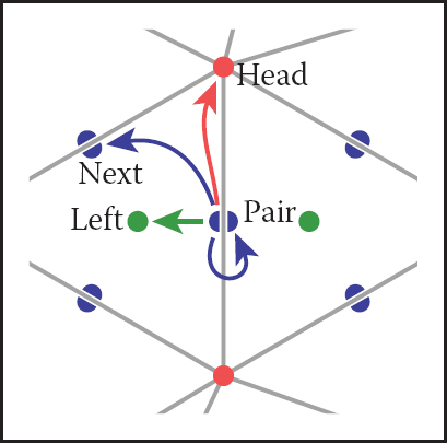
The winged-edge structure is quite elegant, but it has one remaining awkwardness—the need to constantly check which way the edge is oriented before moving to the next edge. This check is directly analogous to the search we saw in the basic version of the triangle neighbor structure: we are looking to find out whether we entered the present edge from the head or from the tail. The solution is also almost indistinguishable: rather than storing data for each edge, we store data for each half-edge. There is one half-edge for each of the two triangles that share an edge, and the two half-edges are oriented oppositely, each oriented consistently with its own triangle.
The data normally stored in an edge is split between the two half-edges. Each half-edge points to the face on its side of the edge and to the vertex at its head, and each contains the edge pointers for its face. It also points to its neighbor on the other side of the edge, from which the other half of the information can be found. Like the winged-edge, a half-edge can contain pointers to both the previous and next half-edges around its face, or only to the next half-edge. We’ll show the example that uses a single pointer.
HEdge {
HEdge pair, next;
Vertex v;
Face f;
}
Face {
// ... per-face data ...
HEdge h; // any h-edge of this face
}
Vertex {
// ... per-vertex data ...
HEdge h; // any h-edge pointing toward this vertex
}
Traversing a half-edge structure is just like traversing a winged-edge structure except that we no longer need to check orientation, and we follow the pair pointer to access the edges in the opposite face.
EdgesOfVertex(v) {
h = v.h;
do {
h = h.pair.next;
} while (h != v.h);
}
EdgesOfFace(f) {
h = f.h;
do {
h = h.next;
} while (h != f.h);
}
The vertex traversal here is clockwise, which is necessary because of omitting the prev pointer from the structure.
Because half-edges are generally allocated in pairs (at least in a mesh with no boundaries), many implementations can do away with the pair pointers. For instance, in an implementation based on array indexing (such as shown in Figure 12.18), the array can be arranged so that an even-numbered edge i always pairs with edge i + 1 and an odd-numbered edge j always pairs with edge j − 1.

In addition to the simple traversal algorithms shown in this chapter, all three of these mesh topology structures can support “mesh surgery” operations of various sorts, such as splitting or collapsing vertices, swapping edges, adding or removing triangles, etc.
12.2 Scene Graphs
A triangle mesh manages a collection of triangles that constitute an object in a scene, but another universal problem in graphics applications is arranging the objects in the desired positions. As we saw in Chapter 6, this is done using transformations, but complex scenes can contain a great many transformations and organizing them well makes the scene much easier to manipulate. Most scenes admit to a hierarchical organization, and the transformations can be managed according to this hierarchy using a scene graph.
To motivate the scene-graph data structure, we will use the hinged pendulum shown in Figure 12.19. Consider how we would draw the top part of the pendulum:

A hinged pendulum. On the left are the two pieces in their “local” coordinate systems. The hinge of the bottom piece is at point b and the attachment for the bottom piece is at its local origin. The degrees of freedom for the assembled object are the angles (θ, ϕ) and the location p of the top hinge.
Apply M3 to all points in upper pendulum
The bottom is more complicated, but we can take advantage of the fact that it is attached to the bottom of the upper pendulum at point b in the local coordinate system. First, we rotate the lower pendulum so that it is at an angle ϕ relative to its initial position. Then, we move it so that its top hinge is at point b. Now it is at the appropriate position in the local coordinates of the upper pendulum, and it can then be moved along with that coordinate system. The composite transform for the lower pendulum is:
Apply Md to all points in lower pendulum
Thus, we see that the lower pendulum not only lives in its own local coordinate system, but also that coordinate system itself is moved along with that of the upper pendulum.
We can encode the pendulum in a data structure that makes management of these coordinate system issues easier, as shown in Figure 12.20. The appropriate matrix to apply to an object is just the product of all the matrices in the chain from the object to the root of the data structure. For example, consider the model of a ferry that has a car that can move freely on the deck of the ferry, and wheels that each move relative to the car as shown in Figure 12.21.


A ferry, a car on the ferry, and the wheels of the car (only two shown) are stored in a scene-graph.
As with the pendulum, each object should be transformed by the product of the matrices in the path from the root to the object:
- ferry transform using M0;
- car body transform using M0M1;
- left wheel transform using M0M1M2;
- left wheel transform using M0M1M3.
An efficient implementation can be achieved using a matrix stack, a data structure supported by many APIs. A matrix stack is manipulated using push and pop operations that add and delete matrices from the right-hand side of a matrix product. For example, calling:
push(M0)
push(M1)
push(M2)
creates the active matrix M = M0M1M2. A subsequent call to pop() strips the last matrix added so that the active matrix becomes M = M0M1. Combining the matrix stack with a recursive traversal of a scene graph gives us:
function traverse(node)
push(Mlocal)
draw object using composite matrix from stack
traverse(left child)
traverse(right child)
pop()
There are many variations on scene graphs but all follow the basic idea above.
12.3 Spatial Data Structures
In many, if not all, graphics applications, the ability to quickly locate geometric objects in particular regions of space is important. Ray tracers need to find objects that intersect rays; interactive applications navigating an environment need to find the objects visible from any given viewpoint; games and physical simulations require detecting when and where objects collide. All these needs can be supported by various spatial data structures designed to organize objects in space so they can be looked up efficiently.
In this section we will discuss examples of three general classes of spatial data structures. Structures that group objects together into a hierarchy are object partitioning schemes: objects are divided into disjoint groups, but the groups may end up overlapping in space. Structures that divide space into disjoint regions are space partitioning schemes: space is divided into separate partitions, but one object may have to intersect more than one partition. Space partitioning schemes can be regular, in which space is divided into uniformly shaped pieces, or irregular, in which space is divided adaptively into irregular pieces, with smaller pieces where there are more and smaller objects.
We will use ray tracing as the primary motivation while discussing these structures, though they can all also be used for view culling or collision detection. In Chapter 4, all objects were looped over while checking for intersections. For N objects, this is an O(N) linear search and is thus slow for large scenes. Like most search problems, the ray-object intersection can be computed in sub-linear time using “divide and conquer” techniques, provided we can create an ordered data structure as a preprocess. There are many techniques to do this.
This section discusses three of these techniques in detail: bounding volume hierarchies (Rubin & Whitted, 1980; Whitted, 1980; Goldsmith & Salmon, 1987), uniform spatial subdivision (Cleary, Wyvill, Birtwistle, & Vatti, 1983; Fujimoto, Tanaka, & Iwata, 1986; Amanatides & Woo, 1987), and binary space partitioning (Glassner, 1984; Jansen, 1986; Havran, 2000). An example of the first two strategies is shown in Figure 12.22.

Left: a uniform partitioning of space. Right: adaptive bounding-box hierarchy.
Image courtesy David DeMarle.
12.3.1 Bounding Boxes
A key operation in most intersection-acceleration schemes is computing the intersection of a ray with a bounding box (Figure 12.23). This differs from conventional intersection tests in that we do not need to know where the ray hits the box; we only need to know whether it hits the box.

To build an algorithm for ray-box intersection, we begin by considering a 2D ray whose direction vector has positive x and y components. We can generalize this to arbitrary 3D rays later. The 2D bounding box is defined by two horizontal and two vertical lines:
The points bounded by these lines can be described in interval notation:
As shown in Figure 12.24, the intersection test can be phrased in terms of these intervals. First, we compute the ray parameter where the ray hits the line x = x min:
![Figure showing the ray will be inside the interval x ∈ [xmin, xmax] for some interval in its parameter space t ∈ [txmin, txmax]. A similar interval exists for the y interval. The ray intersects the box if it is in both the x interval and y interval at the same time, i.e., the intersection of the two one-dimensional intervals is not empty.](http://images-20200215.ebookreading.net/23/1/1/9781482229417/9781482229417__fundamentals-of-computer__9781482229417__image__fig12-24.png)
The ray will be inside the interval x ∈ [xmin, xmax] for some interval in its parameter space t ∈ [txmin, txmax]. A similar interval exists for the y interval. The ray intersects the box if it is in both the x interval and y interval at the same time, i.e., the intersection of the two one-dimensional intervals is not empty.
We then make similar computations for t xmax, tymin, and tymax. The ray hits the box if and only if the intervals [t xmin, txmax] and [tymin, tymax] overlap, i.e., their intersection is nonempty. In pseudocode this algorithm is:
txmin = (xmin − xe)/xd
txmax = (xmax - xe)/xd
tymin = (ymin - ye)/yd
tymax = (ymax - ye)/yd
if (txmin > tymax) or (tymin > txmax) then
return false
else
return true
The if statement may seem non-obvious. To see the logic of it, note that there is no overlap if the first interval is either entirely to the right or entirely to the left of the second interval.
The first thing we must address is the case when xd or yd is negative. If xd is negative, then the ray will hit xmax before it hits xmin. Thus the code for computing txmin and txmax expands to:
if (xd ≥ 0) then
txmin = (xmin − xe)/xd
txmax = (xmax − xe)/xd
else
txmin = (xmax − xe)/xd
txmax = (xmin − xe)/xd
A similar code expansion must be made for the y cases. A major concern is that horizontal and vertical rays have a zero value for yd and xd, respectively. This will cause divide by zero which may be a problem. However, before addressing this directly, we check whether IEEE floating point computation handles these cases gracefully for us. Recall from Section 1.5 the rules for divide by zero: for any positive real number a,
Consider the case of a vertical ray where xd = 0 and yd > 0. We can then calculate
There are three possibilities of interest:
- xe ≤ x min (no hit);
- x min < xe < x max (hit);
- xmax ≤ xe (no hit).
For the first case we have
This yields the interval (txmin, txmin) = (∞, ∞). That interval will not overlap with any interval, so there will be no hit, as desired. For the second case, we have
This yields the interval (txmin, txmin) = (−∞,∞) which will overlap with all intervals and thus will yield a hit as desired. The third case results in the interval (−∞, −∞) which yields no hit, as desired. Because these cases work as desired, we need no special checks for them. As is often the case, IEEE floating point conventions are our ally. However, there is still a problem with this approach.
Consider the code segment:
if (xd > 0) then
tmin = (xmin - xe)/xd
tmax = (xmax - xe)/xd
else
tmin = (xmax − xe)/xd
tmax = (xmin − xe)/xd
This code breaks down when xd = −0. This can be overcome by testing on the reciprocal of xd (A. Williams, Barrus, Morley, & Shirley, 2005):
a = 1/Xd
if (a ≥ 0) then
tmin = a(xmin − xe)
tmax = a(xmax − xe)
else
tmin = a(xmax − xe)
tmax = a(xmin - xe)
12.3.2 Hierarchical Bounding Boxes
The basic idea of hierarchical bounding boxes can be seen by the common tactic of placing an axis-aligned 3D bounding box around all the objects as shown in Figure 12.25. Rays that hit the bounding box will actually be more expensive to compute than in a brute force search, because testing for intersection with the box is not free. However, rays that miss the box are cheaper than the brute force search. Such bounding boxes can be made hierarchical by partitioning the set of objects in a box and placing a box around each partition as shown in Figure 12.26. The data structure for the hierarchy shown in Figure 12.27 might be a tree with the large bounding box at the root and the two smaller bounding boxes as left and right subtrees. These would in turn each point to a list of three triangles. The intersection of a ray with this particular hard-coded tree would be:


The gray box is a tree node that points to the three gray spheres, and the thick black box points to the three black spheres. Note that not all spheres enclosed by the box are guaranteed to be pointed to by the corresponding tree node.
if (ray hits root box) then
if (ray hits left subtree box) then
check three triangles for intersection
if (ray intersects right subtree box) then
check other three triangles for intersection
if (an intersections returned from each subtree) then
return the closest of the two hits
else if (a intersection is returned from exactly one subtree) then
return that intersection
else
return false
else
return false
Some observations related to this algorithm are that there is no geometric ordering between the two subtrees, and there is no reason a ray might not hit both subtrees. Indeed, there is no reason that the two subtrees might not overlap.
A key point of such data hierarchies is that a box is guaranteed to bound all objects that are below it in the hierarchy, but they are not guaranteed to contain all objects that overlap it spatially, as shown in Figure 12.27. This makes this geometric search somewhat more complicated than a traditional binary search on strictly ordered one-dimensional data. The reader may note that several possible optimizations present themselves. We defer optimizations until we have a full hierarchical algorithm.
If we restrict the tree to be binary and require that each node in the tree have a bounding box, then this traversal code extends naturally. Further, assume that all nodes are either leaves in the tree and contain a primitive, or that they contain one or two subtrees.
The bvh-node class should be of type surface, so it should implement surface::hit. The data it contains should be simple:
class bvh-node subclass of surface
virtual bool hit(ray e + td, real t0, real t1, hit-record rec)
virtual box bounding-box()
surface-pointer left
surface-pointer right
box bbox
The traversal code can then be called recursively in an object-oriented style:
function bool bvh-node::hit(ray a + tb, real t0, real t1, hit-record rec)
if (bbox.hitbox(a + tb, t0, t1)) then
hit-record lrec, rrec
left-hit = (left ≠ NULL) and (left → hit(a + tb, t0, t1, lrec))
right-hit = (right ≠ NULL) and (right → hit(a+tb, t0, t1, rrec))
if (left-hit and right-hit) then
if (lrec.t < rrec.t) then
rec = lrec
else
rec = rrec
return true
else if (left-hit) then
rec = lrec
return true
else if (right-hit) then
rec = rrec
return true
else
return false
else
return false
Note that because left and right point to surfaces rather than bvh-nodes specifically, we can let the virtual functions take care of distinguishing between internal and leaf nodes; the appropriate hit function will be called. Note that if the tree is built properly, we can eliminate the check for left being NULL. If we want to eliminate the check for right being NULL, we can replace NULL right pointers with a redundant pointer to left. This will end up checking left twice, but will eliminate the check throughout the tree. Whether that is worth it will depend on the details of tree construction.
There are many ways to build a tree for a bounding volume hierarchy. It is convenient to make the tree binary, roughly balanced, and to have the boxes of sibling subtrees not overlap too much. A heuristic to accomplish this is to sort the surfaces along an axis before dividing them into two sublists. If the axes are defined by an integer with x = 0, y = 1, and z = 2 we have:
function bvh-node::create(object-array A, int AXIS)
N = A.length
if (N= 1) then
left = A[0]
right = NULL
bbox = bounding-box(A[0])
else if (N= 2) then
left-node = A[0]
right-node = A[1]
bbox = combine(bounding-box(A[0]), bounding-box(A[1]))
else
sort A by the object center along AXIS
left= new bvh-node(A[0..N/2 − 1], (AXIS +1) mod 3)
right = new bvh-node(A[N/2..N−1], (AXIS +1) mod 3)
bbox = combine(left → bbox, right → bbox)
The quality of the tree can be improved by carefully choosing AXIS each time. One way to do this is to choose the axis such that the sum of the volumes of the bounding boxes of the two subtrees is minimized. This change compared to rotating through the axes will make little difference for scenes composed of isotopically distributed small objects, but it may help significantly in less well-behaved scenes. This code can also be made more efficient by doing just a partition rather than a full sort.
Another, and probably better, way to build the tree is to have the subtrees contain about the same amount of space rather than the same number of objects. To do this we partition the list based on space:
function bvh-node::create(object-array A, int AXIS)
N = A. length
if (N = 1) then
left = A[0]
right = NULL
bbox = bounding-box(A[0])
else if (N = 2) then
left = A[0]
right = A[1]
bbox = combine(bounding-box(A[0]),bounding-box(A[1]))
else
find the midpoint m of the bounding box of A along AXIS
partition A into lists with lengths k and (N − k) surrounding m
left = new bvh-node(A[0..k], (AXIS +1) mod 3)
right = new bvh-node(A[k + 1..N − 1], (AXIS +1) mod 3)
bbox = combine (left → bbox, right → bbox)
Although this results in an unbalanced tree, it allows for easy traversal of empty space and is cheaper to build because partitioning is cheaper than sorting.
12.3.3 Uniform Spatial Subdivision
Another strategy to reduce intersection tests is to divide space. This is fundamentally different from dividing objects as was done with hierarchical bounding volumes:
- In hierarchical bounding volumes, each object belongs to one of two sibling nodes, whereas a point in space may be inside both sibling nodes.
- In spatial subdivision, each point in space belongs to exactly one node, whereas objects may belong to many nodes.
In uniform spatial subdivision, the scene is partitioned into axis-aligned boxes. These boxes are all the same size, although they are not necessarily cubes. The ray traverses these boxes as shown in Figure 12.28. When an object is hit, the traversal ends.
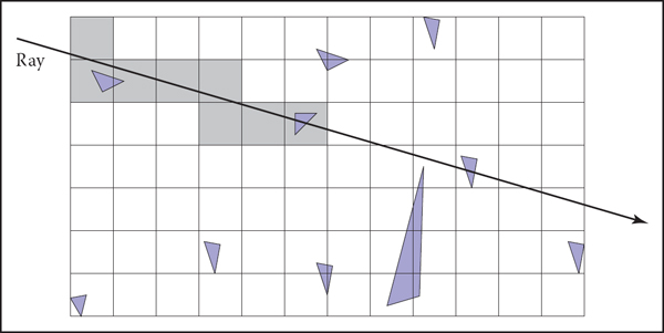
In uniform spatial subdivision, the ray is tracked forward through cells until an object in one of those cells is hit. In this example, only objects in the shaded cells are checked.
The grid itself should be a subclass of surface and should be implemented as a 3D array of pointers to surface. For empty cells these pointers are NULL. For cells with one object, the pointer points to that object. For cells with more than one object, the pointer can point to a list, another grid, or another data structure, such as a bounding volume hierarchy.
This traversal is done in an incremental fashion. The regularity comes from the way that a ray hits each set of parallel planes, as shown in Figure 12.29. To see how this traversal works, first consider the 2D case where the ray direction has positive x and y components and starts outside the grid. Assume the grid is bounded by points (xmin, ymin) and (xmax, ymax). The grid has nx × ny cells.

Although the pattern of cell hits seems irregular (left), the hits on sets of parallel planes are very even.
Our first order of business is to find the index (i, j) of the first cell hit by the ray e + td. Then, we need to traverse the cells in an appropriate order. The key parts to this algorithm are finding the initial cell (i, j) and deciding whether to increment i or j (Figure 12.30). Note that when we check for an intersection with objects in a cell, we restrict the range of t to be within the cell (Figure 12.31). Most implementations make the 3D array of type “pointer to surface.” To improve the locality of the traversal, the array can be tiled as discussed in Section 12.5.

To decide whether we advance right or upward, we keep track of the intersections with the next vertical and horizontal boundary of the cell.

Only hits within the cell should be reported. Otherwise the case above would cause us to report hitting object b rather than object a.
12.3.4 Axis-Aligned Binary Space Partitioning
We can also partition space in a hierarchical data structure such as a binary space partitioning tree (BSP tree). This is similar to the BSP tree used for visibility sorting in Section 12.4, but it’s most common to use axis-aligned, rather than polygon-aligned, cutting planes for ray intersection.
A node in this structure contains a single cutting plane and a left and right subtree. Each subtree contains all the objects on one side of the cutting plane. Objects that pass through the plane are stored in in both subtrees. If we assume the cutting plane is parallel to the yz plane at x = D, then the node class is:
class bsp-node subclass of surface
virtual bool hit(ray e + td, real t0, real t1, hit-record rec)
virtual box bounding-box()
surface-pointer left
surface-pointer right
real D
We generalize this to y and z cutting planes later. The intersection code can then be called recursively in an object-oriented style. The code considers the four cases shown in Figure 12.32. For our purposes, the origin of these rays is a point at parameter t0:

The four cases are:
- The ray only interacts with the left subtree, and we need not test it for intersection with the cutting plane. It occurs for xp < D and xb < 0.
- The ray is tested against the left subtree, and if there are no hits, it is then tested against the right subtree. We need to find the ray parameter at x = D, so we can make sure we only test for intersections within the subtree. This case occurs for xp < D and xb > 0.
- This case is analogous to case 1 and occurs for xp > D and xb > 0.
- This case is analogous to case 2 and occurs for xp > D and xb < 0.
The resulting traversal code handling these cases in order is:
function bool bsp-node::hit(ray a + tb, real t0, real t1, hit-record rec)
xp = xa +t0xb
if (xp < D) then
if (xb < 0) then
return (left ≠ NULL) and (left→hit(a + tb, t0, t1, rec))
t = (D - xa)/xb
if (t>t1) then
return (left ≠ NULL) and (left→hit(a + tb, t0, t1, rec))
if (left ≠ NULL) and (left→hit(a + tb, t0, t, rec)) then
return true return (right ≠ NULL) and (right→hit(a + tb, t, t1, rec))
else
analogous code for cases 3 and 4
This is very clean code. However, to get it started, we need to hit some root object that includes a bounding box so we can initialize the traversal, t0 and t1. An issue we have to address is that the cutting plane may be along any axis. We can add an integer index axis to the bsp-node class. If we allow an indexing operator for points, this will result in some simple modifications to the code above, for example,
would become
which will result in some additional array indexing, but will not generate more branches.
While the processing of a single bsp-node is faster than processing a bvh-node, the fact that a single surface may exist in more than one subtree means there are more nodes and, potentially, a higher memory use. How “well” the trees are built determines which is faster. Building the tree is similar to building the BVH tree. We can pick axes to split in a cycle, and we can split in half each time, or we can try to be more sophisticated in how we divide.
12.4 BSP Trees for Visibility
Another geometric problem in which spatial data structures can be used is determining the visibility ordering of objects in a scene with changing viewpoint.
If we are making many images of a fixed scene composed of planar polygons, from different viewpoints—as is often the case for applications such as games— we can use a binary space partitioning scheme closely related to the method for ray intersection discussed in the previous section. The difference is that for visibility sorting we use non—axis-aligned splitting planes, so that the planes can be made coincident with the polygons. This leads to an elegant algorithm known as the BSP tree algorithm to order the surfaces from front to back. The key aspect of the BSP tree is that it uses a preprocess to create a data structure that is useful for any viewpoint. So, as the viewpoint changes, the same data structure is used without change.
12.4.1 Overview of BSP Tree Algorithm
The BSP tree algorithm is an example of a painter’s algorithm. A painter’s algorithm draws every object from back-to-front, with each new polygon potentially overdrawing previous polygons, as is shown in Figure 12.33. It can be implemented as follows:

A painter’s algorithm starts with a blank image and then draws the scene one object at a time from back-to-front, overdrawing whatever is already there. This automatically eliminates hidden surfaces.
sort objects back to front relative to viewpoint
for each object do
draw object on screen
The problem with the first step (the sort) is that the relative order of multiple objects is not always well defined, even if the order of every pair of objects is. This problem is illustrated in Figure 12.34 where the three triangles form a cycle.
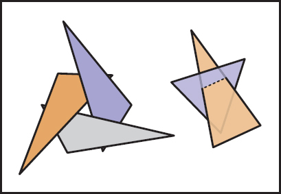
A cycle occurs if a global back-to-front ordering is not possible for a particular eye position.
The BSP tree algorithm works on any scene composed of polygons where no polygon crosses the plane defined by any other polygon. This restriction is then relaxed by a preprocessing step. For the rest of this discussion, triangles are assumed to be the only primitive, but the ideas extend to arbitrary polygons.
The basic idea of the BSP tree can be illustrated with two triangles, T1 and T2. We first recall (see Section 2.5.3) the implicit plane equation of the plane containing T1: f1(p) = 0. The key property of implicit planes that we wish to take advantage of is that for all points p+ on one side of the plane, f1(p+) > 0; and for all points p− on the other side of the plane, f1(p−) < 0. Using this property, we can find out on which side of the plane T2 lies. Again, this assumes all three vertices of T2 are on the same side of the plane. For discussion, assume that T2 is on the f1(p) < 0 side of the plane. Then, we can draw T1 and T2 in the right order for any eyepoint e:
if (f1(e) < 0) then
draw T1
draw T2
else
draw T2
draw T1
The reason this works is that if T2 and e are on the same side of the plane containing T1, there is no way for T2 to be fully or partially blocked by T1 as seen from e, so it is safe to draw T1 first. If e and T2 are on opposite sides of the plane containing T1, then T2 cannot fully or partially block T1, and the opposite drawing order is safe (Figure 12.35).

When e and T2 are on opposite sides of the plane containing T1, then it is safe to draw T2 first and T1 second. If e and T2 are on the same side of the plane, then T1 should be drawn before T2. This is the core idea of the BSP tree algorithm.
This observation can be generalized to many objects provided none of them span the plane defined by T1. If we use a binary tree data structure with T1 as root, the negative branch of the tree contains all the triangles whose vertices have fi(p) < 0, and the positive branch of the tree contains all the triangles whose vertices have fi(p) > 0. We can draw in proper order as follows:
function draw(bsptree tree, point e)
if (tree.empty) then
return
if (ftree.root(e) < 0) then
draw(tree.plus, e)
rasterize tree.triangle
draw(tree.minus, e)
else
draw(tree.minus, e)
rasterize tree.triangle
draw(tree.plus, e)
The nice thing about that code is that it will work for any viewpoint e, so the tree can be precomputed. Note that, if each subtree is itself a tree, where the root triangle divides the other triangles into two groups relative to the plane containing it, the code will work as is. It can be made slightly more efficient by terminating the recursive calls one level higher, but the code will still be simple. A tree illustrating this code is shown in Figure 12.36. As discussed in Section 2.5.5, the implicit equation for a point p on a plane containing three non-colinear points a, b, and c is

Three triangles and a BSP tree that is valid for them. The “positive” and “negative” are encoded by right and left subtree position, respectively.
It can be faster to store the (A, B, C, D) of the implicit equation of the form
Equations (12.1) and (12.2) are equivalent, as is clear when you recall that the gradient of the implicit equation is the normal to the triangle. The gradient of Equation (12.2) is n = (A, B, C) which is just the normal vector
We can solve for D by plugging in any point on the plane, e.g., a:
which is the same as Equation (12.1) once you recall that n is computed using the cross product. Which form of the plane equation you use and whether you store only the vertices, n and the vertices, or n, D, and the vertices, is probably a matter of taste—a classic time-storage tradeoff that will be settled best by profiling. For debugging, using Equation (12.1) is probably the best.
The only issue that prevents the code above from working in general is that one cannot guarantee that a triangle can be uniquely classified on one side of a plane or the other. It can have two vertices on one side of the plane and the third on the other. Or it can have vertices on the plane. This is handled by splitting the triangle into smaller triangles using the plane to “cut” them.
12.4.2 Building the Tree
If none of the triangles in the dataset cross each other’s planes, so that all triangles are on one side of all other triangles, a BSP tree that can be traversed using the code above can be built using the following algorith
tree-root = node(T1)
for i∈{2,..., N} do
tree-root.add(Ti)
function add (triangle T)
if (f(a) < 0 and f(b) < 0 and f(c) < 0) then
if (negative subtree is empty) then
negative-subtree = node(T)
else
negative-subtree.add (T)
else if (f(a) > 0 and f(b) > 0 and f(c) > 0) then
if positive subtree is empty then
positive-subtree = node(T)
else
positive-subtree.add(T)
else
we have assumed this case is impossible
The only thing we need to fix is the case where the triangle crosses the dividing plane, as shown in Figure 12.37. Assume, for simplicity, that the triangle has vertices a and b on one side of the plane, and vertex c is on the other side. In this case, we can find the intersection points A and B and cut the triangle into three new triangles with vertices

When a triangle spans a plane, there will be one vertex on one side and two on the other.
as shown in Figure 12.38. This order of vertices is important so that the direction of the normal remains the same as for the original triangle. If we assume that f(c) < 0, the following code could add these three triangles to the tree assuming the positive and negative subtrees are not empty:

When a triangle is cut, we break it into three triangles, none of which span the cutting plane.
A precision problem that will plague a naive implementation occurs when a vertex is very near the splitting plane. For example, if we have two vertices on one side of the splitting plane and the other vertex is only an extremely small distance on the other side, we will create a new triangle almost the same as the old one, a triangle that is a sliver, and a triangle of almost zero size. It would be better to detect this as a special case and not split into three new triangles. One might expect this case to be rare, but because many models have tessellated planes and triangles with shared vertices, it occurs frequently, and thus must be handled carefully. Some simple manipulations that accomplish this are:
function add(triangle T)
fa = f(a)
fb = f(b)
fc = f(c)
if (abs(fa) < ε) then
fa = 0
if (abs(fb) < ε) then
fb = 0
if (abs(fc) < ε) then
fc = 0
if (fa ≤ 0 and fb ≤ 0 and fc ≤ 0) then
if (negative subtree is empty) then
negative-subtree = node(T)
else
negative-subtree.add(T)
else if (fa ≥ 0 and fb ≥ 0 and fc ≥ 0) then
if (positive subtree is empty) then
positive-subtree = node(T)
else
positive-subtree.add(T)
else
cut triangle into three triangles and add to each side
This takes any vertex whose f value is within e of the plane and counts it as positive or negative. The constant e is a small positive real chosen by the user. The technique above is a rare instance where testing for floating-point equality is useful and works because the zero value is set rather than being computed. Comparing for equality with a computed floating-point value is almost never advisable, but we are not doing that.
12.4.3 Cutting Triangles
Filling out the details of the last case “cut triangle into three triangles and add to each side” is straightforward, but tedious. We should take advantage of the BSP tree construction as a preprocess where highest efficiency is not key. Instead, we should attempt to have a clean compact code. A nice trick is to force many of the cases into one by ensuring that c is on one side of the plane and the other two vertices are on the other. This is easily done with swaps. Filling out the details in the final else statement (assuming the subtrees are nonempty for simplicity) gives:
if (fa * fc ≥ 0) then
swap(fb, fc)
swap(b, c)
swap(fa, fb)
swap(a, b)
else if (fb * fc ≥ 0) then
swap(fa, fc)
swap(a, c)
swap(fa, fb)
swap(a, b)
compute A
compute B
T 1 = (a, b, A)
T2 = (b, B, A)
T3 = (A, B, c)
if (fc ≥ 0) then
negative-subtree.add(T1)
negative-subtree.add(T2)
positive-subtree.add(T3)
else
positive-subtree.add(T1)
positive-subtree.add(T2)
negative-subtree.add(T3)
This code takes advantage of the fact that the product of a and b are positive if they have the same sign—thus, the first if statement. If vertices are swapped, we must do two swaps to keep the vertices ordered counterclockwise. Note that exactly one of the vertices may lie exactly on the plane, in which case the code above will work, but one of the generated triangles will have zero area. This can be handled by ignoring the possibility, which is not that risky, because the rasterization code must handle zero-area triangles in screen space (i.e., edge-on triangles). You can also add a check that does not add zero-area triangles to the tree. Finally, you can put in a special case for when exactly one of fa, fb, and fc is zero which cuts the triangle into two triangles.
To compute A and B, a line segment and implicit plane intersection is needed. For example, the parametric line connecting a and c is
The point of intersection with the plane n · p + D = 0 is found by plugging p(t) into the plane equation:
and solving for t:
Calling this solution tA, we can write the expression for A:
A similar computation will give B.
12.4.4 Optimizing the Tree
The efficiency of tree creation is much less of a concern than tree traversal because it is a preprocess. The traversal of the BSP tree takes time proportional to the number of nodes in the tree. (How well balanced the tree is does not matter.) There will be one node for each triangle, including the triangles that are created as a result of splitting. This number can depend on the order in which triangles are added to the tree. For example, in Figure 12.39, if T1 is the root, there will be two nodes in the tree, but if T2 is the root, there will be more nodes, because T1 will be split.

Using T1 as the root of a BSP tree will result in a tree with two nodes. Using T2 as the root will require a cut and thus make a larger tree.
It is difficult to find the “best” order of triangles to add to the tree. For N triangles, there are N! orderings that are possible. So trying all orderings is not usually feasible. Alternatively, some predetermined number of orderings can be tried from a random collection of permutations, and the best one can be kept for the final tree.
The splitting algorithm described above splits one triangle into three triangles. It could be more efficient to split a triangle into a triangle and a convex quadrilateral. This is probably not worth it if all input models have only triangles, but would be easy to support for implementations that accommodate arbitrary polygons.
12.5 Tiling Multidimensional Arrays
Effectively utilizing the memory hierarchy is a crucial task in designing algorithms for modern architectures. Making sure that multidimensional arrays have data in a “nice” arrangement is accomplished by tiling, sometimes also called bricking. A traditional 2D array is stored as a 1D array together with an indexing mechanism; for example, an Nx by Ny array is stored in a 1D array of length NxNy and the 2D index (x, y) (which runs from (0, 0) to (Nx −1, Ny −1)) maps to the 1D index (running from 0 to NxNy − 1) using the formula
An example of how that memory lays out is shown in Figure 12.40. A problem with this layout is that although two adjacent array elements that are in the same row are next to each other in memory, two adjacent elements in the same column will be separated by Nx elements in memory. This can cause poor memory locality for large Nx. The standard solution to this is to use tiles to make memory locality for rows and columns more equal. An example is shown in Figure 12.41 where 2 × 2 tiles are used. The details of indexing such an array are discussed in the next section. A more complicated example, with two levels of tiling on a 3D array, is covered after that.


The memory layout for a tiled 2D array with Nx = 4 and Ny = 3 and 2 × 2 tiles. Note that padding on the top of the array is needed because Ny is not a multiple of the tile size two.
A key question is what size to make the tiles. In practice, they should be similar to the memory-unit size on the machine. For example, if we are using 16-bit (2-byte) data values on a machine with 128-byte cache lines, 8 × 8 tiles fit exactly in a cache line. However, using 32-bit floating-point numbers, which fit 32 elements to a cache line, 5 × 5 tiles are a bit too small and 6 × 6 tiles are a bit too large. Because there are also coarser-sized memory units such as pages, hierarchical tiling with similar logic can be useful.
12.5.1 One-Level Tiling for 2D Arrays
If we assume an Nx×Ny array decomposed into square n×n tiles (Figure 12.42), then the number of tiles required is

Here, we assume that n divides Nx and Ny exactly. When this is not true, the array should be padded. For example, if Nx = 15 and n = 4, then Nx should be changed to 16. To work out a formula for indexing such an array, we first find the tile indices (bx, by) that give the row/column for the tiles (the tiles themselves form a 2D array):
where ÷ is integer division, e.g., 12 ÷ 5 = 2. If we order the tiles along rows as shown in Figure 12.40, then the index of the first element of the tile (bx, by) is
The memory in that tile is arranged like a traditional 2D array as shown in Figure 12.41. The partial offsets (x', y') inside the tile are
where mod is the remainder operator, e.g., 12 mod 5 = 2. Therefore, the offset inside the tile is
Thus the full formula for finding the 1D index element (x, y) in an Nx × Ny array with n × n tiles is
This expression contains many integer multiplication, divide and modulus operations, which are costly on some processors. When n is a power of two, these operations can be converted to bitshifts and bitwise logical operations. However, as noted above, the ideal size is not always a power of two. Some of the multiplications can be converted to shift/add operations, but the divide and modulus operations are more problematic. The indices could be computed incrementally, but this would require tracking counters, with numerous comparisons and poor branch prediction performance.
However, there is a simple solution; note that the index expression can be written as
where
We tabulate Fx and Fy, and use x and y to find the index into the data array. These tables will consist of Nx and Ny elements, respectively. The total size of the tables will fit in the primary data cache of the processor, even for very large data set sizes.
12.5.2 Example: Two-Level Tiling for 3D Arrays
Effective TLB utilization is also becoming a crucial factor in algorithm performance. The same technique can be used to improve TLB hit rates in a 3D array by creating m × m × m bricks of n × n × n cells. For example, a 40 × 20 × 19 volume could be decomposed into 4 × 2 × 2 macrobricks of 2 × 2 × 2 bricks of 5 × 5 × 5 cells. This corresponds to m = 2 and n = 5. Because 19 cannot be factored by mn = 10, one level of padding is needed. Empirically useful sizes are m = 5 for 16-bit datasets and m = 6 for float datasets.
The resulting index into the data array can be computed for any (x, y, z) triple with the expression
where Nx, Ny and Nz are the respective sizes of the dataset.
Note that, as in the simpler 2D one-level case, this expression can be written as
where
Frequently Asked Questions
- Does tiling really make that much difference in performance?
On some volume rendering applications, a two-level tiling strategy made as much as a factor-of-ten performance difference. When the array does not fit in main memory, it can effectively prevent thrashing in some applications such as image editing.
- How do I store the lists in a winged-edge structure?
For most applications, it is feasible to use arrays and indices for the references. However, if many delete operations are to be performed, then it is wise to use linked lists and pointers.
Notes
The discussion of the winged-edge data structure is based on the course notes of Ching-Kuang Shene (Shene, 2003). There are smaller mesh data structures than winged-edge. The tradeoffs in using such structures is discussed in Directed Edges—A Scalable Representation for Triangle Meshes (Campagna, Kobbelt, & Seidel, 1998). The tiled-array discussion is based on Interactive Ray Tracing for Volume Visualization (S. Parker et al., 1999). A structure similar to the triangle neighbor structure is discussed in a technical report by Charles loop (loop, 2000). A discussion of manifolds can be found in an introductory topology text (Munkres, 2000).
Exercises
- What is the memory difference for a simple tetrahedron stored as four independent triangles and one stored in a winged-edge data structure?
- Diagram a scene graph for a bicycle.
- How many look-up tables are needed for a single-level tiling of an n-dimensional array?
- Given N triangles, what is the minimum number of triangles that could be added to a resulting BSP tree? What is the maximum number?